Abstract

The CP symmetry is a fundamental discrete symmetry in chiral gauge theory. Therefore this symmetry is expected to be kept also on the lattice. However, it has been pointed out by Hasenfratz that the chiral fermion action in Lüscher’s formulation of lattice chiral gauge theory is not invariant under CP transformation. In this thesis, we first review the method of constructing chiral gauge theory on the lattice. Then we generalize the analysis of Hasenfratz and show that CP symmetry is not manifestly implemented for the local and doubler-free Ginsparg-Wilson operator under rather general assumptions for chiral projection operators. We next calculate the fermion generating functional and precisely identify where the effects of this CP breaking appear in this formulation. We show that they appear in: (I) Overall constant phase of the fermion generating functional. (II) Overall dimensionful constant of the fermion generating functional. (III)Fermion propagator appearing in external fermion lines and the propagator connected to Yukawa vertices. The first effect appears from the transformation of the path integral measure and it is absorbed into a suitable definition of the constant phase factor for each topological sector; in this sense there appears no “CP anomaly”. The second constant arises from the explicit breaking in the action and it is absorbed by the suitable weights with which topological sectors are summed. The last one in the propagator is inherent to this formulation. This breaking emerges as an (almost) contact term in the propagator when the Higgs field, which is treated perturbatively, has no vacuum expectation value. In the presence of the vacuum expectation value, however, a completely new situation arises and the breaking becomes intrinsically non-local. This non-local CP breaking is expected to persist for a non-perturbative treatment of the Higgs coupling. The basics of lattice gauge theory are briefly summarized in Appendix.A.

Chapter 1 Introduction

Lattice gauge theory has been the most successful tool to calculate various physical quantities in gauge theory in the strong coupling region since it was proposed by Wilson in 1974 [1]. Lattice gauge theory is defined on a discrete Euclidean space-time which provides a non-perturbative regularization scheme. An ultra-violet cutoff is given by the inverse of the lattice spacing. Lattice gauge theory in finite volume is also a good starting point for the constructive quantum field theory, since neither ultra-violet divergences nor infrared divergences exist there. An important feature of lattice gauge theory is to enable the numerical analysis of gauge theory with the computer by using the method similar to those used for the statistical mechanics systems. Until now, various physical quantities in low energy QCD, hadron masses, quark masses, string tension and so on, which we can not calculate in perturbation theory, have been calculated by the numerical method. 

While gauge fields can be latticized as link variables excellently, the problem, which is so-called the fermion doubling problem, appears when one tries to put fermions on the lattice [3]. In particular, it was considered to be difficult that one puts a massless fermion on the lattice because of the Nielsen-Ninomiya no-go theorem [4]. However, the recent progress in the treatment of the fermion, which began with the domain-wall fermion [5, 6], has enabled us to put the massless fermion on the lattice. Dirac operators which describe a single massless fermion have been discovered, for example, the overlap Dirac operator [7] derived from the overlap formalism [8, 9] and the fixed point action through renormalization group approaches. While these Dirac operators are derived through quite different procedures, they satisfy the Ginsparg-Wilson relation [11]. Moreover, Lüscher pointed out that the Ginsparg-Wilson relation is equivalent to a lattice chiral symmetry [12]. See refs. [13]–[17] for reviews on this progress. As for the numerical aspects, the numerical analysis of the weak matrix elements concerning the CP breaking parameter $\epsilon^{\prime}/\epsilon$ band $\Delta I=1/2$ rule in the Standard Model has made significant progress recently in the formulation of QCD with the domain-wall fermion [18]-[20], though the definite results have not been obtained yet.

The Standard Model which describes the behaviour of elementary particles at present is a chiral gauge theory [21]. In chiral gauge theory left-handed fermions and right-handed fermions belong to different gauge-group representations. A peculiar feature of chiral gauge theory is the appearance of the gauge anomaly, which is the breaking of gauge symmetry by quantum effects. Whether gauge anomalies appear or not depends on the gauge group and the fermion multiplet. The theory with such anomalies has no meaning, since such anomalies break the fundamental principles in the theory, for example, unitarity of S matrix. Therefore we have to consider a theory where all of the possible anomalies cancell. In perturbation theory it has been shown that there exist no gauge anomalies to all orders in gauge couplings, if gauge anomalies cancel at one-loop level. Further conditions, however, may be needed to keep gauge symmetry at the non-perturbative level. For example, the chiral gauge theory with an odd number of Weyl fermion multiplets in SU(2) fundamental representation has no anomalies in perturbation theory. At the non-perturbative level, however, the global anomaly, which is called the Witten anomaly [23, 24], appears and thus this theory is inconsistent.

In chiral gauge theory another problem is the regularization problem. The appearance of gauge anomalies implies that the gauge-invariant regularization is possible only when the multiplets of Weyl fermions are anomaly-free. Therefore, the gauge-invariant regularization should be directly related to the fermion representation of the gauge group. The standard regularization schemes, for example, dimensional regularization, Pauli-Villars method and so on, are not quite convenient to analyze the gauge symmetry in chiral gauge theory. If a more fundamental gauge-invariant regularization scheme is established, it may simplify the calculations of radiative corrections in electroweak processes.

The recent progress in lattice gauge theory has led us also to the exciting possibilities for constructing non-perturbative chiral gauge theory with exact gauge invariance [25]-[34]. The construction of lattice chiral gauge theory with exact gauge invariance is called Lüscher’s formulation, which is adopted in this thesis. In Lüscher’s formulation with the Ginsparg-Wilson operators, anomaly-free $U(1)$ chiral gauge theory in finite volume [25]   and electroweak $SU(2)\times U(1)$ chiral gauge theory [29] in infinite volume have been constructed on the lattice. The global anomaly is also analyzed on the lattice [32, 33]. Further, in perturbation theory chiral gauge theories with exact gauge invariance are constructed on the lattice to all orders of the gauge coupling for general anomaly-free gauge group [30]. In addition, a programme for the construction of chiral gauge theories with general anomaly-free gauge groups in a non-perturbative manner has been proposed [27]. Therefore, the numerical analysis of the Standard Model, such as, the investigation of the behaviour of elctroweak phase transition at finite temperature, is coming to be possible. This construction of lattice chiral gauge theory will also deepen our understanding of chiral gauge theory in the strong coupling region.

It has been however pointed out by Hasenfratz that the chiral fermion action in this formulation is not invariant under CP transformation [38], if one uses the ordinary lattice chiral projectors [39, 13]. CP symmetry is a fundamental discrete symmetry in chiral gauge theory and hence is expected to be kept on the lattice. This peculiar feature of lattice chiral gauge theory may influence the lattice analysis of the Standard Model which keeps CP symmetry except a phase factor in CKM matrix. Therefore it is very important to examine the detailed breaking of CP symmetry in this formulation.

In this thesis the breaking of CP symmetry in lattice chiral gauge theory will be examined on the basis of two papers [40, 41]. In Chapter 2 we will review the formulation of lattice chiral gauge theory in detail, following refs. [25, 27]. In Chapter 3, Hasenfratz’s analysis is extended, utilizing more general projection operators [40]. Then we will show that the CP breaking in chiral fermion action persists under the standard CP transformation, even if one utilizes a general class of Ginsparg-Wilson operators which are local and free of species doublers and utilizes rather general chiral projections. The CP breaking is thus regarded as an inherent feature of this class of formulation. Therefore, we will next examine this CP breaking at the quantum level by calculating the fermion generating functional [41]. Then we will show that the effects of CP violation emerge only at: (I) Overall constant phase of the fermion generating functional. (II) Overall dimensionful constant of the fermion generating functional. (III) Fermion propagator appearing in external fermion lines and the propagator connected to Yukawa vertices. Our result is summarized in eq. (3.95) for pure chiral gauge theory and, when there is a Yukawa coupling, in eq. (3.108). The first two constants above depend only on the topological sectors concerned and the problem is reduced to the choice of weights with which various topological sectors are summed. This problem, which is not particular to this formulation, is thus fixed by a suitable choice of weight factors. The last effect in the fermion propagator, on the other hand, can not be removed. When the Higgs field has no expectation value, it emerges as an (almost) contact term. However, in the presence of the Higgs expectation value, this breaking becomes intrinsically non-local. In Chapter 4, we will summarize our result and give a few remarks.

Chapter 2 Lattice chiral gauge theory

In this chapter Lüscher’s formulation of lattice chiral gauge theory is presented [25, 27]. We first discuss the lattice Dirac operator used in this formulation. Next, Weyl fermions are defined, utilizing the chiral projection operators. The definition of the fermion integration measure is non-trivial, however, and there exists the freedom of the phase of the measure. The conditions for fixing the phase, so that the formulation satisfies gauge invariance and all other fundamental principle , is summarized in Lüscher’s reconstruction theorem.

2.1 Lattice Dirac operator

We first consider the Dirac fermion and the projection to the left-handed components is discussed in the next section.

We consider a general form of the Ginsparg-Wilson relation. In terms of the hermitian operator $H$: 

$$H=a\gamma_{5}D=aD^{\dagger}\gamma_{5}=H^{\dagger},$$ (2.3)

this relation is written as

$$\gamma_{5}H+H\gamma_{5}=2H^{2}f(H^{2}),$$ (2.4)

where $f(H^{2})$ is a regular function of $H^{2}$ and $f(H^{2})^{\dagger}=f(H^{2})$. For simplicity, we assume that $f(x)$ is monotonous and non-decreasing for $x\geq 0$. The simplest choice $f(H^{2})=1$ corresponds to the conventional Ginsparg-Wilson relation (A.31). The properties of $H$ for $f(H^{2})=H^{2k}$ with a positive integer $k$ have been investigated [42]-[46]. As an important consequence of eq.(2.4), one has

$$\gamma_{5}H^{2}=(\gamma_{5}H+H\gamma_{5})H-H(\gamma_{5}H+H\gamma_{5})+H^{2}\gamma_{5}=H^{2}\gamma_{5},$$ (2.6)

which implies $DH^{2}=H^{2}D$. The combination

$$\Gamma_{5}=\gamma_{5}-Hf(H^{2}),$$ (2.7)

has a special role due to the property

$$\Gamma_{5}H+H\Gamma_{5}=0.$$ (2.8)

Moreover, the above defining relation (2.4) is written in a variety of ways such as

$$\gamma_{5}\Gamma_{5}\gamma_{5}D+D\Gamma_{5}=0,$$

$$\gamma_{5}H+H\hat{\gamma}_{5}=0,\ \ \ \gamma_{5}D+D\hat{\gamma}_{5}=0,$$ (2.9)

and $\hat{\gamma}^{2}_{5}=1$ where

$$\hat{\gamma}_{5}=\gamma_{5}-2Hf(H^{2}),$$ (2.10)

which is the modified chiral matrix  [13, 39]. In this thesis we assume that the lattice Dirac operator satisfies the above general Ginsparg-Wilson relation and has no doublers. We also assume that $D$ is local and has the smooth dependence with respect to link variables.

2.1.1 Admissibility condition and the index theorem

The locality and smoothness have been established for the overlap Dirac operator [47, 48], if the plaquette variables satisfy the admissibility condition:

$$\|1-R[U_{\mu\nu}(x)]\|<\epsilon,\qquad\mbox{for all plaquettes},$$ (2.11)

where $R$ is the representation of the gauge group  and $\epsilon$ is a fixed positive number. We assume this condition also when we use Dirac operators satisfying the general Ginsparg-Wilson relation (2.4), since this restriction gives the topological structure to the space of link variables [49, 50]. If there is no restriction on link variables, any link variables can be continuously deformed to the trivial field $U_{\mu}(x)=1$ on the lattice and thus there is no topological structure.

Now we define the topological charge to establish the index theorem on the lattice. For this purpose, we first discuss lattice chiral symmetry [12]. The fermion action which has the Dirac operator satisfying the general Ginsparg-Wilson relation (2.4) is invariant under the global transformation:

$$\psi(x)\to\psi^{\prime}(x)=\psi(x)+i\epsilon^{a}T^{a}\hat{\gamma}_{5}\psi(x),$$

$$\bar{\psi}(x)\to\bar{\psi}^{\prime}(x)=\bar{\psi}(x)+i\epsilon^{a}\bar{\psi}(x)\gamma_{5}T^{a},$$ (2.12)

on account of the relation (2.1) and where $T^{a}$ are flavor-matrices. But the fermion measure produces the Jacobian factor:

$${\cal D}\bar{\psi}^{\prime}{\cal D}\psi^{\prime}=J{\cal D}\bar{\psi}{\cal D}\psi,$$

$$J=\mbox{exp}(-2i\epsilon\mathop{\rm Tr}\nolimits(\Gamma_{5}T^{a})).$$ (2.13)

From this expression, we see that the fermion measure is invariant under the non-singlet flavor transformation, but not for the flavor-singlet transformation, which agrees with the continuum theory [51]. $\mathop{\rm Tr}\nolimits\Gamma_{5}$ is regarded as the chiral anomaly on the lattice. Therefore we may define the topological charge on the lattice as $Q=\mathop{\rm Tr}\nolimits\Gamma_{5}$ . Now we can show the index theorem on the lattice by examining the representation of the algebra (2.4) [42]. From the analysis in Appendix B, $\mathop{\rm Tr}\nolimits\Gamma_{5}$ is written as follows($n=0$ stands for $\lambda_{n}=0$),

$$\mathop{\rm Tr}\nolimits\Gamma_{5} \equiv \sum_{n}\left(\varphi_{n},\Gamma_{5}\varphi_{n}\right)$$ (2.14)

$$= \sum_{n=0}\left(\varphi_{n},\Gamma_{5}\varphi_{n}\right)$$

$$= \sum_{n=0}\left(\varphi_{n},\gamma_{5}\varphi_{n}\right)=n_{+}-n_{-}=\>\mbox{index}.$$

This is the index theorem on the lattice [52]. Since $\Gamma_{5}$ depends smoothly on the link variable within the space of admissible configurations (2.11), the integer $n_{+}-n_{-}$ is a constant in a connected component of the space of admissible configurations; $n_{+}-n_{-}$ thus provides a topological characterization of the gauge field configuration, i.e., the index .

Therefore the admissibility condition (2.11) has important roles in the formulation with the Ginsparg-Wilson relation. The one role is that it ensures the locality and smoothness of the lattice Dirac operator. Another role is that it gives rise to the topological structure in the space of link variables.

2.1.2 Gauge field action

In this subsection let us mention the gauge field action in this formulation. To impose the restriction on the space of link variables, which is caused by the admissibility condition, we may take a gauge field action which is different from the standard Wilson action (A.4). For example,

$$S_{G}=\left\{\begin{array}[]{ll}\displaystyle\frac{1}{g_{0}^{2}}a^{4}\sum_{x,\mu\neq\nu}\frac{\mathop{\rm Tr}\nolimits\left(1-U_{\mu\nu}(x)\right)}{1-\|1-U_{\mu\nu}(x)\|^{2}/\epsilon^{2}},&\quad\mbox{if $\|1-U_{\mu\nu}\|<\epsilon$},\\ \infty&\quad\mbox{otherwise}.\end{array}\right.$$ (2.22)

Note that $S_{G}$ is local and a smooth function of the link variables and satisfies gauge invariance. In particular, the functional integral can be constructed in the usual way with the standard integration measure

2.2 Lattice chiral gauge theory

In this section, we analyze the case of pure chiral gauge theory without Higgs couplings. The extension to the case with Higgs couplings is straightforward and it will be discussed in Section 3.4.

2.2.1 Weyl fermion

To make the following discussion as general as possible, we introduce a one-parameter family of lattice analog of $\gamma_{5}$:

$$\gamma_{5}^{(t)}={\gamma_{5}-tHf(H^{2})\over\sqrt{1+t(t-2)H^{2}f^{2}(H^{2})}}.$$ (2.24)

Note that $\gamma_{5}^{(0)}=\gamma_{5}$ and, when $f(H^{2})=1$, $\gamma_{5}^{(2)}=\hat{\gamma}_{5}$ corresponds to the conventional modified chiral matrix (2.10). Note that $\gamma_{5}^{(1)}=\Gamma_{5}/\sqrt{\Gamma_{5}^{2}}$. The “conjugate” of $\gamma_{5}^{(t)}$ is defined by

$$\overline{\gamma}_{5}^{(t)}=\gamma_{5}\gamma_{5}^{(2-t)}\gamma_{5},$$ (2.25)

and they satisfy the following relations:

$$\gamma_{5}^{(t)\dagger}=\gamma_{5}^{(t)},\qquad\overline{\gamma}_{5}^{(t)\dagger}=\overline{\gamma}_{5}^{(t)},\qquad(\gamma_{5}^{(t)})^{2}=(\overline{\gamma}_{5}^{(t)})^{2}=1,$$

$$\overline{\gamma}_{5}^{(t)}D+D\gamma_{5}^{(t)}=0.$$ (2.26)

In view of the last relation in (2.26), we may introduce the chiral projection operators by

$$P_{\pm}^{(t)}={1\over 2}(1\pm\gamma_{5}^{(t)}),\qquad\overline{P}_{\pm}^{(t)}={1\over 2}(1\pm\overline{\gamma}_{5}^{(t)}),$$ (2.27)

so that

$$\overline{P}_{\pm}^{(t)}D=DP_{\mp}^{(t)}.$$ (2.28)

Then the left-handed Weyl fermion is defined by

$$P_{-}^{(t)}\psi=\psi,\qquad\overline{\psi}\overline{P}_{+}^{(t)}=\overline{\psi}.$$ (2.29)

The kinetic term is then consistently decomposed according to the chirality:

$$D=\overline{P}_{+}^{(t)}DP_{-}^{(t)}+\overline{P}_{-}^{(t)}DP_{+}^{(t)}.$$ (2.30)

2.2.2 Fermion integration measure

To define the fermion integration measure, we introduce certain orthonormal vectors in the constrained space,

$$P_{-}^{(t)}v_{j}(x)=v_{j}(x),\qquad\overline{v}_{k}\overline{P}_{+}^{(t)}(x)=\overline{v}_{k}(x),$$

$$\left(v_{j},v_{k}\right)=\delta_{jk},\qquad\left(\bar{v}_{j}^{\dagger},\bar{v}_{k}^{\dagger}\right)=\delta_{jk},$$ (2.31)

and expand the fields as

$$\psi(x)=\sum_{j}v_{j}(x)c_{j},\qquad\overline{\psi}(x)=\sum_{k}\overline{c}_{k}\overline{v}_{k}(x).$$ (2.32)

Then the (ideal) integration measure is defined by

$${\rm D}[\psi]{\rm D}[\overline{\psi}]=\prod_{j}{\rm d}c_{j}\prod_{k}{\rm d}\overline{c}_{k}.$$ (2.33)

The condition (2.31) shows that the basis vectors may depend on the link variable because the chiral projectors depend on it. However, this conditions alone do not determine how the basis vectors depend on the link variables. We first note the identity

$$\delta_{\xi}v_{j}=P_{-}^{(t)}\delta_{\xi}v_{j}+(1-P_{-}^{(t)})\delta_{\xi}v_{j},$$ (2.34)

where $\delta_{\xi}v_{j}$ is the variation of basis under an infinitesimal variation of the link variables,

$$\delta_{\xi}U_{\mu}(x)=a\xi_{\mu}(x)U_{\mu}(x),\qquad\xi_{\mu}(x)=\xi_{\mu}^{a}(x)T^{a},$$ (2.35)

with $\xi_{\mu}^{a}(x)$ being any real vector field and then note that the constraint (2.31) implies

$$(1-P_{-}^{(t)})\delta_{\xi}v_{j}=\delta_{\xi}P_{-}^{(t)}v_{j}.$$ (2.36)

Consequently, the second term of the variation $\delta_{\xi}v_{j}$, $(1-P_{-}^{(t)})\delta_{\xi}v_{j}$, is fixed uniquely by (2.36). However, the component of $\delta_{\xi}v_{j}$ residing in the constrained space, $P_{-}^{(t)}\delta_{\xi}v_{j}$, is not determined by the constraint (2.31). This fact means that the fermion measure is not specified uniquely and there is an ambiguity of the phase. One can see this by noting that when one changes basis by unitary transformation matrices ${\cal Q}$ and $\bar{{\cal Q}}$ as

$$v_{j}^{\prime}(x)=\sum_{l}v_{l}(x){\cal Q}_{lj},\qquad c_{j}^{\prime}(x)=\sum_{l}{\cal Q}^{-1}_{jl}c_{l},$$

$$\bar{v}_{j}^{\prime}(x)=\sum_{l}\bar{{\cal Q}}_{jl}\bar{v}_{l}(x),\qquad\bar{c}_{j}^{\prime}=\sum_{l}\bar{c}_{l}\bar{{\cal Q}}^{-1}_{lj},$$ (2.37)

the fermion measure changes as follows,

$${\rm D}[\psi]{\rm D}[\overline{\psi}]^{\left\{v^{\prime},\bar{v}^{\prime}\right\}}=\det{\cal Q}\det\bar{{\cal Q}}{\rm D}[\psi]{\rm D}[\overline{\psi}]^{\left\{v,\bar{v}\right\}},$$ (2.38)

where ${\rm D}[\psi]{\rm D}[\overline{\psi}]^{\left\{..,..\right\}}$ stands for the measure defined by the basis in the curly bracket and where $\det{\cal Q}$ and $\det\bar{{\cal Q}}$ are pure phase factors, which may depend on the link variables since the basis vectors depend on the link variables. Thus the fermion measure has the freedom of the phase which may depend on the link variables. How to fix this phase will be discussed later. For the time being we assume that some particular choice of the basis has been made. The above general setup, which is closely related to the overlap formulation in refs. [8, 9], does not specify the formulation uniquely, leaving the phase unspecified.

Correlation functions and the effective action

We have just defined the Weyl fermion and the fermion measure(except the freedom of the phase of the fermion integration measure). Now we can describe the path-integral expression of the expectation value of an operator ${\cal O}$ [25, 27]:

$$\langle{\cal O}\rangle={1\over{\cal Z}}\sum_{M}\int_{M}{\rm D}[U]\,e^{-S_{G}}{\cal N}_{M}e^{i\vartheta_{M}}\langle{\cal O}\rangle_{\rm F}^{M},$$ (2.39)

where $M$ denotes the topological sector specified by the admissibility (2.11). The “topological weight”, ${\cal N}_{M}e^{i\vartheta_{M}}$, with which the topological sectors are summed, is not fixed within this formulation. In each topological sector $M$, the average with respect to the fermion fields $\langle{\cal O}\rangle_{\rm F}^{M}$ is defined by the generating functional of fermion Green’s functions

$$Z_{\rm F}[U,\eta,\overline{\eta};t]=\int{\rm D}[\psi]{\rm D}[\overline{\psi}]\,e^{-S_{\rm F}},$$ (2.40)

where we have written the dependence on the parameter $t$ in eq. (2.24) explicitly  and

$$S_{\rm F}=a^{4}\sum_{x}[\overline{\psi}(x)D\psi(x)-\overline{\psi}(x)\eta(x)-\overline{\eta}(x)\psi(x)],$$ (2.41)

where $\eta(x)$ and $\bar{\eta}(x)$ are source fields. The fermion integration variables are subject to the chirality constraint (2.29).

Now we can work out a few quantities in this formalism.

• Fermion propagator
  If $D$ has not zero modes, we obtain

  $$\frac{\langle\psi(x)\bar{\psi}(y)\rangle}{\langle 1\rangle_{\rm F}} = P_{-}^{(t)}\frac{1}{D}\bar{P}_{+}^{(t)}.$$ (2.42)

  The correlation functions with arbitrary products of fermions can be calculated by Wick’s theorem.

• Effective action
  In the vacuum sector the effective action without source fields is given by

  $$\langle 1\rangle_{\rm F}=\det M,\qquad M_{kj}=a^{4}\sum_{x}\overline{v}_{k}(x)Dv_{j}(x).$$ (2.43)

  Its link variable variation is given by

  $$\delta_{\xi}\ln\det M=\mathop{\rm Tr}\nolimits(\delta_{\xi}DP_{-}^{(t)}D^{-1}\overline{P}_{+}^{(t)})-i{\cal L}_{\xi},$$ (2.44)

  where

  $${\cal L}_{\xi}[U;t]=i\sum_{j}\left(v_{j},\delta_{\xi}v_{j}\right)+i\sum_{k}(\delta_{\xi}\overline{v}_{k}^{\dagger},\overline{v}_{k}^{\dagger}).$$ (2.45)

  This term appears because the basis vectors $\{v,\bar{v}\}$ depend on the link variables. In addition, under the basis transformations (2.2.2) this term transforms as follows,

  $${\cal L}_{\xi}^{\{v^{\prime},\bar{v}^{\prime}\}}={\cal L}_{\xi}^{\{v,\bar{v}\}}+i\delta_{\xi}\ln\,\det{\cal Q}+i\delta_{\xi}\ln\,\det\bar{{\cal Q}}.$$ (2.46)

  This transformation law means that ${\cal L}_{\xi}[U;t]$ is a quantity associated with the fermion measure and we call this term the “measure term”. Since the measure term is purely imaginary, it contributes only to the imaginary part of eq. (2.44):

  $${1\over 2}[\mathop{\rm Tr}\nolimits(\delta_{\xi}DP_{-}^{(t)}D^{-1}\overline{P}_{+}^{(t)})-\mathop{\rm Tr}\nolimits(\delta_{\xi}DP_{-}^{(t)}D^{-1}\overline{P}_{+}^{(t)})^{*}]$$

  $$={1\over 2}[\mathop{\rm Tr}\nolimits(\delta_{\xi}DP_{-}^{(t)}D^{-1})-\mathop{\rm Tr}\nolimits(\delta_{\xi}DP_{+}^{(2-t)}D^{-1})]$$

  $$=-{1\over 4}\mathop{\rm Tr}\nolimits\delta_{\xi}D(\gamma_{5}^{(t)}+\gamma_{5}^{(2-t)})D^{-1},$$ (2.47)

  where we have used eq. (2.1) and eq. (2.25). The measure term is then chosen to improve the imaginary part of the effective action (see, for example, ref. [26]).

  The measure term can be rewritten, when we take the linearity of the measure term on $\xi_{\mu}(x)$ into account, as follows,

  $${\cal L}_{\xi}=a^{4}\sum_{x}\xi_{\mu}^{a}(x)j_{\mu}^{a}(x).$$ (2.48)

  with a current $j_{\mu}^{a}(x)$. In the following subsection this current associated with the measure plays an important role.

2.2.3 Lüscher’s reconstruction theorem

Let us return to the problem of how to fix the phase of the fermion measure which has been unspecified. We should find a basis in eq. (2.33) or the associated measure term for which the gauge invariance (assuming the fermion multiplet is anomaly-free) and the locality are ensured for finite lattice spacings in this formulation. Lüscher has showed that chiral gauge theories with anomaly-free multiplets of Weyl fermions can be put on the lattice without violating the fundamental principles if several conditions on the current $j_{\mu}(x)$ associated with the measure term are satisfied, which is called “Lüscher’s reconstruction theorem” [25, 27].

Lüscher’s reconstruction theorem

The formulation of the chiral gauge theory with anomaly-free fermions on the lattice is local and smooth on the link variables and has gauge invariance, if the current $j_{\mu}(x)$ satisfies the following conditions.

i)locality and smoothness

$j_{\mu}(x)$ is local and is smoothly dependent on the link variables.

ii)gauge invariance

$j_{\mu}(x)$ is gauge-covariant and satisfies the “anomalous conservation law”:

$$(\nabla_{\mu}^{*}j_{\mu})^{a}(x) = {\cal A}^{a}(x)$$

$${\cal A}^{a}(x) = -{i\over 2}\mathop{\rm tr}\nolimits R(T^{a})(\gamma_{5}^{(t)}+\gamma_{5}^{(2-t)})(x,x).$$ (2.51)

iii)integrability

$j_{\mu}(x)$ satisfies the “integrability condition”: Along all closed curves in the space of the link variables $U^{\tau}_{\mu}(x)$ ($0\leq\tau\leq 1$), Wilson lines which are made of $j_{\mu}(x)$ satisfy the following equation:

$$W = \exp\biggl{(}i\int_{0}^{1}{\rm d}\tau\,{\cal L}_{\xi}\biggr{)},\quad a\xi_{\mu}(x)=\partial_{\tau}U^{\tau}_{\mu}(x)U^{\tau}_{\mu}(x)^{-1},$$

$$= \det(1-P_{0}^{(t)}+P_{0}^{(t)}Q_{1}^{(t)})\det\nolimits(1-P_{0}^{(2-t)}+P_{0}^{(2-t)}Q_{1}^{(2-t)}),$$

where $P_{\tau}^{(t)}=P_{-}^{(t)}|_{U=U_{\tau}}$ and $\overline{P}_{\tau}^{(t)}=\overline{P}_{+}^{(t)}|_{U=U_{\tau}}$. The unitary operator $Q_{\tau}^{(t)}$ in this expression is defined by

$$\partial_{\tau}Q_{\tau}^{(t)}={1\over 4}[\partial_{\tau}\gamma_{\tau}^{(t)},\gamma_{\tau}^{(t)}]Q_{\tau}^{(t)},\qquad Q_{0}^{(t)}=1,$$ (2.53)

where $\gamma_{\tau}^{(t)}=\gamma_{5}^{(t)}|_{U=U_{\tau}}$.

The current $j_{\mu}(x)$ which has above properties is called an “ideal current”. The next crucial task is to find out an ideal current. For $\mathop{\rm{}U}(1)$ theories, such a current was constructed by Lüscher [25]. For electroweak $\mathop{\rm SU}(2)\times\mathop{\rm{}U}(1)$ theory also, such a current has been constructed on the infinite volume lattice [29]. For general non-abelian theories, the measure from an ideal current has been constructed only in perturbation theory [30, 28], but the existence of such an ideal fermion measure in non-perturbative level has not been established yet(except for the real representation of the gauge group [31]). In such a case it seems necessary to clarify the topological structure of the space of the admissible link variables but this task remains to be performed.

We will discuss more details of the contents of the above theorem in the following subsections.

Locality and smoothness

We first require that the expectation value of the products of fermionic and link variables (2.39) should be smooth functions of the link variable. This requirement is necessary to derive the field equation discussed below.

The locality is one of the most important properties in lattice theory. The universality in the continuum limit depends on this property. To ensure the locality in this formulation, it is necessary to require the locality of field equation. The field equation is obtained by calculating the change of (2.39) under the variations of the link variables (2.35). When ${\cal O}$ does not contain fermion fields, we obtain

$$\langle\{\delta_{\xi}S_{G}+\sum_{x}\bar{\psi}(x)\delta_{\xi}D\psi(x)+i{\cal L}_{\xi}\}{\cal O}\rangle=\langle\delta_{\xi}{\cal O}\rangle.$$ (2.54)

In this equation the first two terms are clearly local owing to the locality of the action. We thus need to require that ${\cal L}_{\xi}$, therefore, $j_{\mu}(x)$ should be local functions of the link variable to ensure the locality of field equation , as stated in i) in above theorem.

Gauge invariance

The gauge invariance also is an important property which has to be required in this formulation. In particular, the fermion effective action should be gauge-invariant. Now the gauge transformation is given by (2.35) with

$$\xi_{\mu}(x) = -\nabla_{\mu}\omega(x)$$ (2.55)

$$= \-{1\over a}[U_{\mu}(x)\omega(x+a\hat{\mu})U_{\mu}(x)^{-1}-\omega(x)].$$

Noting the transformation property of the Dirac operator:

$$\delta_{\xi}D=\left\{R(w),D\right\},$$ (2.56)

the gauge variation of the expectation value is written as follows,

$$\delta_{\xi}\langle{\cal O}\rangle_{\rm F}=\langle\delta_{\xi}{\cal O}\rangle_{\rm F}+ia^{4}\sum_{x}\omega^{a}(x)[{\cal A}^{a}(x)-(\nabla_{\mu}^{*}j_{\mu})^{a}(x)]\langle{\cal O}\rangle_{\rm F},$$

$${\cal A}^{a}(x)=-{i\over 2}\mathop{\rm tr}\nolimits R(T^{a})(\gamma_{5}^{(t)}+\gamma_{5}^{(2-t)})(x,x),$$ (2.57)

where ${\cal A}^{a}(x)$ can be regarded as the covariant anomaly on the lattice. Hence, for the gauge invariant formulation, the current $j_{\mu}(x)$ should satisfy the “anomalous conservation law”:

$$(\nabla_{\mu}^{*}j_{\mu})^{a}(x)={\cal A}^{a}(x),$$ (2.58)

and it should be also gauge-covariant because of the gauge invariance of the effective action and (2.44), as stated in ii).

Integrability condition

To obtain the fermion measure from a given current $j_{\mu}(x)$, we need the integrability of a current. Here, we show that the fermion measure can be constructed from $j_{\mu}(x)$ which satisfies a certain integrability condition.

To derive the integrability condition, we consider the change of the phase of the fermion effective action under the smooth curves in the space of link variable:

$$U^{\tau}_{\mu}(x),\qquad 0\leq\tau\leq 1.$$ (2.59)

Then the change of the phase of the effective action is represented as Wilson line:

$$W = \exp\biggl{(}i\int_{0}^{1}{\rm d}\tau\,{\cal L}_{\xi}\biggr{)},\quad a\xi_{\mu}(x)=\partial_{\tau}U^{\tau}_{\mu}(x)U^{\tau}_{\mu}(x)^{-1}.$$ (2.60)

We first calculate the Wilson line with a basis $\left\{v,\bar{v}\right\}$ along a closed curve, assuming that this basis is smoothly defined on the space of admissible link variables. To describe this we introduce the projectors

$$P_{\tau}^{(t)}=P_{-}^{(t)}|_{U=U^{\tau}},\qquad\overline{P}_{\tau}^{(t)}=\overline{P}_{+}^{(t)}|_{U=U^{\tau}},$$ (2.61)

and define the unitary operators $Q_{\tau}$ through

$$\partial_{\tau}Q_{\tau}^{(t)}=[\partial_{\tau}P_{\tau}^{(t)},P_{\tau}^{(t)}]Q_{\tau}^{(t)},\qquad Q_{0}^{(t)}=1,$$ (2.62)

From this, we have (See Appendix C)

$$P_{\tau}^{(t)}=Q_{\tau}^{(t)}P_{0}^{(t)}Q_{\tau}^{(t)\dagger},\qquad\overline{P}_{\tau}^{(t)}=\gamma_{5}Q_{\tau}^{(2-t)}\gamma_{5}\overline{P}_{0}^{(t)}(\gamma_{5}Q_{\tau}^{(2-t)}\gamma_{5})^{\dagger}.$$ (2.63)

Therefore $Q_{\tau}$ is the transporter of $P_{\tau}$ along the curve. After some calculations(Appendix C), the Wilson line with the smooth basis is obtained as follows,

$$W = \det(1-P_{0}^{(t)}+P_{0}^{(t)}Q_{1}^{(t)})\det\nolimits^{-1}(1-\overline{P}_{0}^{(t)}+\overline{P}_{0}^{(t)}\gamma_{5}Q_{1}^{(2-t)}\gamma_{5})$$ (2.64)

$$= \det(1-P_{0}^{(t)}+P_{0}^{(t)}Q_{1}^{(t)})\det\nolimits(1-P_{0}^{(2-t)}+P_{0}^{(2-t)}Q_{1}^{(2-t)}),$$

along all closed curves, for which $U^{1}=U^{0}$.

Now let $j_{\mu}(x)$ be the smooth function of the admissible link variables. That $j_{\mu}(x)$ should satisfy the above equation (2.64) is clearly the necessary condition to obtain the fermion measure from the current $j_{\mu}(x)$. Moreover, this equation is also the sufficient condition and we can now prove the Lüscher’s reconstruction theorem as follows.

Proof of the reconstruction theorem
Now we assume that we have found an ideal current $j_{\mu}(x)$. The proof is given by an explicit construction of the basis. We may set the fermionic basis vectors for the gauge field $U$ as

$$v_{j}=\cases{Q_{1}^{(t)}u_{1}W^{-1},&for $j=1$,\cr Q_{1}^{(t)}u_{j},&otherwise,\cr}\qquad\overline{v}_{k}=\overline{u}_{k}(\gamma_{5}Q_{1}^{(2-t)}\gamma_{5})^{\dagger},$$ (2.65)

where $u_{j}$ and $\overline{u}_{k}$ are fixed bases defined for the reference configuration $U^{0}$. The vectors are then transported by the operators $Q_{\tau}^{(t)}$ and $Q_{\tau}^{(2-t)}$ along a certain curve connecting $U^{0}$ and $U=U^{1}$. The Wilson line $W$ is also defined along this curve. The above basis depends on the curve chosen, but the associated measure does not, because of eq. (2.64). We can show this as follows. We first consider the two basis, $\left\{v,\bar{v}\right\}$ and $\left\{\tilde{v},\tilde{\bar{v}}\right\}$, which are defined along two curves, $U^{\tau}$ and $\tilde{U}^{\tau}$, which have the same start $U^{0}$ and end $U=U^{1}$, respectively  (2.1).

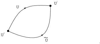
Figure 2.1: Two curves in the space of link variables

Explicitly, $\left\{v,\bar{v}\right\}$ are given by eq.(2.65) and $\left\{\tilde{v},\tilde{\bar{v}}\right\}$ are given by

$$\tilde{v}_{j}=\cases{\tilde{Q}_{1}^{(t)}u_{1}\tilde{W}^{-1},&for $j=1$,\cr\tilde{Q}_{1}^{(t)}u_{j},&otherwise,\cr}\qquad\tilde{\overline{v}}_{k}=\overline{u}_{k}(\gamma_{5}\tilde{Q}_{1}^{(2-t)}\gamma_{5})^{\dagger},$$ (2.66)

where $\tilde{W}$ is constructed from $\tilde{Q}_{1}^{(t)}$ and $\tilde{Q}_{1}^{(2-t)}$ corresponding to the curve $\tilde{U}$. Now the change of the two fermion measures which are constructed from two bases is given by

$${\rm D}[\psi]{\rm D}[\overline{\psi}]^{\left\{v,\bar{v}\right\}} = \det\left\{(\tilde{v}_{j},v_{k})\right\}\det\left\{(\bar{v}_{j}^{\dagger},\tilde{\bar{v}}_{k}^{\dagger})\right\}{\rm D}[\psi]{\rm D}[\overline{\psi}]^{\left\{\tilde{v},\tilde{\bar{v}}\right\}}$$

$$= \left(\tilde{W}^{-1}W\right)^{-1}\det\left\{(u_{j},\tilde{Q}_{1}^{(t)\dagger}Q_{1}^{(t)}u_{k})\right\}$$

$$\times\det\left\{(\bar{u}_{j}^{\dagger},(\gamma_{5}\tilde{Q}_{1}^{(2-t)\dagger}Q_{1}^{(2-t)}\gamma_{5})^{\dagger}\bar{u}_{k}^{\dagger})\right\}{\rm D}[\psi]{\rm D}[\overline{\psi}]^{\left\{\tilde{v},\tilde{\bar{v}}\right\}}.$$

When we define a Wilson line $\tilde{\tilde{W}}$ and $\tilde{\tilde{Q}}_{1}^{(t)}$ for a closed curve $\tilde{\tilde{U}}^{\tau}$ constructed from $U$ and $\tilde{U}^{-1}$ in fig.(2.2),

Figure 2.2: Closed curve in the space of link variables

we have

$$\tilde{\tilde{W}}=\tilde{W}^{-1}W,\qquad\tilde{\tilde{Q}}_{1}^{(t)}=\tilde{Q}_{1}^{(t)\dagger}Q_{1}^{(t)},$$ (2.68)

from the definition of Wilson line (2.60) and the transporter of projection operators (2.62). Then the change of two measures is given by

$$\det\left\{(\tilde{v}_{j},v_{k})\right\}\det\left\{(\bar{v}_{j}^{\dagger},\tilde{\bar{v}}_{k}^{\dagger})\right\}$$

$$\qquad=\det\nolimits^{-1}(1-P_{0}^{(t)}+P_{0}^{(t)}\tilde{\tilde{Q}}_{1}^{(t)})\det\nolimits^{-1}(1-P_{0}^{(2-t)}+P_{0}^{(2-t)}\tilde{\tilde{Q}}_{1}^{(2-t)})$$

$$\qquad\quad\times\det\nolimits(1-P_{0}^{(t)}+P_{0}^{(t)}\tilde{\tilde{Q}}_{1}^{(t)})\det\nolimits(1-P_{+0}^{(2-t)}+P_{+0}^{(2-t)}\tilde{\tilde{Q}}_{1}^{(2-t)\dagger})$$

$$\qquad=1.$$ (2.69)

Thus the measure is path-independent.

We next compute the measure term (2.45) for the above basis (2.65). Under $\left.\delta_{\xi}U_{\mu}^{\tau}(x)=\partial_{\tau}U_{\mu}^{\tau}(x)\right|_{\tau=1}$, the variations of bases are given by

$$\delta_{\xi}v_{j}=\cases{\left[\partial_{\tau}P_{\tau}^{(t)}|_{\tau=1},P_{1}^{(t)}\right]Q_{1}^{(t)}u_{1}W^{-1}\cr\qquad-iQ_{1}^{(t)}u_{1}\left(a^{4}\sum_{y}\xi_{\mu}^{a}(y)j_{\mu}^{a}(y)\right)W^{-1},&\mbox{for $j=1$},\cr\cr\left[\partial_{\tau}P_{\tau}^{(t)}|_{\tau=1},P_{1}^{(t)}\right]Q_{1}^{(t)}u_{j},&\mbox{otherwise},\cr}$$ (2.70)

and

$$\delta_{\xi}\bar{v}_{k}=\bar{u}_{k}(\gamma_{5}Q_{1}^{(2-t)}\gamma_{5})^{\dagger}\left(\left[\partial_{\tau}\bar{P}_{\tau}^{(t)}|_{\tau=1},\bar{P}_{1}^{(t)}\right]\right)^{\dagger},$$ (2.71)

where we used

$$\partial_{\tau}(\gamma_{5}Q_{\tau}^{(2-t)}\gamma_{5})=[\partial_{\tau}\bar{P}_{\tau}^{(t)},\bar{P}_{\tau}^{(t)}]\gamma_{5}Q_{\tau}^{(2-t)}\gamma_{5},$$ (2.72)

which is derived from (2.62). When we substitute these expressions for the variations of the bases in (2.45), we obtain

$${\cal L}_{\xi}^{\{v,\bar{v}\}}=a^{4}\sum_{x}\xi_{\mu}^{a}(x)j_{\mu}^{a}(x),$$ (2.73)

utilizing that $u_{j}(x)$ are orthonormal vectors. Since the ideal current $j_{\mu}^{a}(x)$ satisfies conditions (i) and (ii), the formulation is local and gauge invariant.
In this chapter we have discussed the construction of lattice chiral gauge theory with the exact gauge invariance. In the next chapter, we discuss the effect of CP breaking in this formulation by simply assuming the existence of such an ideal measure. The properties of an ideal basis, which is summarized in Lüscher’s reconstruction theorem, play a crucial role in our following analysis.

Chapter 3 CP breaking in lattice chiral gauge theories

In this chapter we discuss CP breaking in Lüscher’s formulation of lattice chiral gauge theory. We first show that the chiral fermion action with a local and doubler-free Ginsparg-Wilson operator has no CP symmetry under rather mild assumptions for projection operators [40]. We next calculate the fermion generating functional and investigate where the effects of CP breaking appear in this formulation with projection operators (2.27)[41].

3.1 Lattice CP problem in chiral fermion action

In this section we discuss the breaking of CP symmetry in chiral fermion action. We first define C, P, CP transformations on the lattice. Next, we generalize the analysis of Hasenfratz [38] and show that CP breaking is an inherent feature of this formulation.

3.1.1 C, P and CP symmetry on the lattice

In this subsection we discuss C, P and CP transformations in this order. From now on, we assume that the vector-like theory with a Dirac operator which satisfy the general Ginsparg-Wilson relation (2.4) is invariant under the standard C, P, and CP transformations. The Wilson fermion action (A.18) has these discrete symmetries as shown below. Therefore, the above assumption is correct for the action with the Dirac operators which are constructed out of the Wilson-Dirac operators, for instance, for the action of the overlap Dirac operator (A.34). We will also show that this assumption is consistent with the general Ginsparg-Wilson relation (2.4).

Charge conjugation

We denote the charge conjugation by C. The charge conjugation is defined by 

$$\psi(x)\to-C^{-1}\overline{\psi}^{T}(x),\qquad\overline{\psi}(x)\to\psi^{T}(x)C,$$

$$U_{\mu}(x)\to U^{\rm C}_{\mu}(x)=U_{\mu}(x)^{*},$$ (3.1)

where the charge conjugation matrix $C=\gamma_{2}\gamma_{4}$ satisfies

$$C^{\dagger}C=1,\qquad C^{T}=-C,\qquad C\gamma_{\mu}C^{-1}=-\gamma_{\mu}^{T},\qquad C\gamma_{5}C^{-1}=\gamma_{5}^{T}.$$ (3.2)

Now the Wilson fermion action (A.18) transforms under this charge conjugation as follows,

$$\to a^{4}\sum_{x,\mu}\frac{1}{2a}\psi^{T}(x)\left[-C\gamma_{\mu}C^{-1}\left(U_{\mu}^{*}(x)\bar{\psi}^{T}(x+a\hat{\mu})\right.\right.$$ (3.3)

$$\left.\qquad\qquad\qquad\qquad\qquad-U_{\mu}^{T}(x-a\hat{\mu})\bar{\psi}^{T}(x-a\hat{\mu})\right)$$

$$\left.\quad-r\left(2\bar{\psi}^{T}(x)-U_{\mu}^{*}(x)\bar{\psi}^{T}(x+a\hat{\mu})-U_{\mu}^{T}(x-a\hat{\mu})\bar{\psi}^{T}(x-a\hat{\mu})\right)\right]$$

$$\quad-\frac{m_{0}}{a}\psi^{T}(x)\bar{\psi}^{T}(x)$$

$$=(S_{F}^{(W)})^{T}=S_{F}^{(W)}.$$

Therefore, the Wilson fermion action is invariant under the charge conjugation.

This invariance of the action can be represented in terms of the kernel of the Wilson-Dirac operator $D_{W}(x,y)$ as follows,

$$D_{W}(U^{C})(x,y)=C^{-1}D_{W}(U^{C})(x,y)^{T}C,$$ (3.4)

where the transpose operation $T$ acts not only on the matrices involved but also on the arguments as $(x,y)\to(y,x)$. The kernel of the Dirac operator similarly transforms as

$$D(U^{\rm C})(x,y)=C^{-1}D(U)(x,y)^{T}C.$$ (3.5)

Moreover we then have

$$H(U^{\rm C})(x,y)=C^{-1}(\gamma_{5}H(U)(x,y)\gamma_{5})^{T}C,$$

$$H(U^{\rm C})(x,y)^{2}=C^{-1}(H(U)(x,y)^{2})^{T}C.$$ (3.6)

From this transformation laws, we see that the charge conjugation (3.1.1) is consistent with the general Ginsparg-Wilson relation (2.4).

Parity transformation

We denote P the parity transformation by P:

$$x=(x_{i},x_{4})\stackrel{{\scriptstyle P}}{{\to}}\bar{x}=(-x_{i},x_{4}),$$ (3.7)

where $i=1,2,3$. The parity transformation for the fields is defined by

$$\psi(x)\to\gamma_{4}\psi(\bar{x}),\qquad\overline{\psi}(x)\to\overline{\psi}(\bar{x})\gamma_{4},$$

$$U_{\mu}(x)\to U^{\rm P}_{\mu}(x)=\cases{U_{i}(\bar{x}-a\hat{i})^{-1},&for $\mu=i$,\cr U_{4}(\bar{x}),&for $\mu=4$,\cr}.$$ (3.8)

Under this parity transformation, the Wilson fermion action transforms as

$$\to a^{4}\sum_{x,\mu}\frac{1}{2a}\bar{\psi}(\bar{x})\left[\gamma_{4}\gamma_{i}\gamma_{4}\left(U_{i}^{\dagger}(\bar{x}-a\hat{i})\psi(\bar{x}-a\hat{i})-U_{i}^{\dagger}(\bar{x})\psi(\bar{x}+a\hat{i})\right)\right.$$

$$\qquad\qquad+\gamma_{4}\left(U_{4}(\bar{x})\psi(\bar{x}+a\hat{4})-U_{4}^{\dagger}(\bar{x})\psi(\bar{x}-a\hat{4})\right)$$

$$\qquad\qquad+r\left(2\psi(\bar{x})-U_{i}^{\dagger}(\bar{x}-a\hat{i})\psi(\bar{x}-a\hat{i})-U_{i}(\bar{x})\psi(\bar{x}+a\hat{i})\right)$$

$$\qquad\qquad\left.+r\left(-U_{4}(\bar{x})\psi(\bar{x}+a\hat{4})-U_{4}^{\dagger}(\bar{x}-a\hat{4})\psi(\bar{x}-a\hat{4})\right)\right]$$

$$\qquad\qquad+\frac{m_{0}}{a}\bar{\psi}(\bar{x})\psi(\bar{x})$$

$$=S_{F}^{(W)},$$ (3.9)

where we used $\sum_{x}=\sum_{\bar{x}}$. Therefore, the Wilson fermion action satisfies P symmetry and the kernel of the Dirac operator transforms as follows,

$$D(U^{\rm P})(x,y)=\gamma_{4}D(U)(\bar{x},\bar{y})\gamma_{4}.$$ (3.10)

under the parity transformation. Further, we have

$$H(U^{\rm P})(x,y)=-\gamma_{4}H(U)(\bar{x},\bar{y})\gamma_{4},$$

$$H(U^{\rm P})(x,y)^{2}=\gamma_{4}H(U)(\bar{x},\bar{y})^{2}\gamma_{4}.$$ (3.11)

Therefore this parity transformation is consistent with the general Ginsparg-Wilson relation (2.4).

CP transformation

CP transformation interchanges the fermion and anti-fermion. Combining the charge conjugation with the parity transformation, CP transformation is written as follows,

$$\psi(x)\to-W^{-1}\overline{\psi}^{T}(\bar{x}),\qquad\overline{\psi}(x)\to\psi^{T}(\bar{x})W$$

$$U_{\mu}(x)\to U^{\rm CP}_{\mu}(x)=\cases{{U_{i}(\bar{x}-a\hat{i})^{-1}}^{*},&for $\mu=i$,\cr U_{4}(\bar{x})^{*},&for $\mu=4$,\cr}$$ (3.12)

where

$$W=\gamma_{2},\qquad W^{\dagger}W=1,$$

$$W\gamma_{\mu}W^{-1}=\cases{\gamma_{i}^{T},&for $\mu=i$,\cr-\gamma_{4}^{T},&for $\mu=4$,\cr}\qquad W\gamma_{5}W^{-1}=-\gamma_{5}^{T},$$ (3.13)

and thus CP acts on the plaquette variables $U_{\mu\nu}(x)$ as ($\varphi_{ij}(\bar{x}-a\hat{i}-a\hat{j})=U_{j}(\bar{x}-a\hat{i}-a\hat{j})^{*}U_{i}(\bar{x}-a\hat{i})^{*}$)

$$U_{ij}(x)$$

$$\to U^{\rm CP}_{ij}(x)=\varphi_{ij}(\bar{x}-a\hat{i}-a\hat{j})^{-1}U_{ij}(\bar{x}-a\hat{i}-a\hat{j})^{*}\varphi_{ij}(\bar{x}-a\hat{i}-a\hat{j}),$$

$$U_{i4}(x)\to U^{\rm CP}_{i4}(x)={U_{i}(\bar{x}-a\hat{i})^{*}}^{-1}{U_{i4}(\bar{x}-a\hat{i})^{-1}}^{*}U_{i}(\bar{x}-a\hat{i})^{*}.$$ (3.14)

Of course, we can show explicitly that the Wilson fermion action is invariant under this CP transformation and we also have

$$D(U^{\rm CP})(x,y)=W^{-1}D(U)(\bar{x},\bar{y})^{T}W.$$ (3.15)

See Appendix D for the CP transformation properties of various operators.

3.1.2 Lattice CP problem

It has been pointed out that the CP symmetry, the fundamental discrete symmetry in chiral gauge theories, is not manifestly implemented in the Lüscher’s formulation of lattice chiral gauge theory. The basic observation related to this effect is as follows [38]: In the formulation, the chirality is imposed through [39, 13]

$$P_{-}\psi=\psi,\qquad\overline{\psi}\overline{P}_{+}=\overline{\psi},$$ (3.16)

where $\overline{P}_{\pm}=(1\pm\gamma_{5})/2$ and $P_{\pm}=(1\pm\hat{\gamma}_{5})/2$ with $\hat{\gamma}_{5}=\gamma_{5}(1-2aD)$. However, since the above condition is not symmetric in the fermion and anti-fermion and since CP exchanges these two, CP symmetry is explicitly broken. In fact, the fermion action in the case of pure chiral gauge theory without Higgs couplings changes under CP transformation (3.1.1) as follows

$$S_{\rm F}=a^{4}\sum_{x}\overline{\psi}(x)\overline{P}_{+}DP_{-}\psi(x)\to S_{\rm F}=a^{4}\sum_{x}\overline{\psi}(x)\gamma_{5}P_{+}\gamma_{5}D\overline{P}_{-}\psi(x),$$ (3.17)

and this causes the change in the propagator

$${\langle\psi(x)\overline{\psi}(y)\rangle_{\rm F}\over\langle 1\rangle_{\rm F}}=P_{-}{1\over D}\overline{P}_{+}(x,y),$$

$$\to{\langle\psi(x)\overline{\psi}(y)\rangle_{\rm F}\over\langle 1\rangle_{\rm F}}=\overline{P}_{-}{1\over D}\gamma_{5}P_{+}\gamma_{5}(x,y)$$

$$\qquad\qquad=P_{-}{1\over D}\overline{P}_{+}(x,y)-a\gamma_{5}a^{-4}\delta_{x,y}.$$ (3.18)

One might think that a suitable modification of the chiral projectors would remedy this CP breaking. But this is impossible with the standard CP transformation law (3.1.1). The CP invariant chiral fermion action with a local and doubler-free Ginsparg-Wilson operator inevitably contains singularities and hence is non-local. We will show this below [40]. This proof will be performed in two steps. At the first step, we show that the projection operators are limited to particular forms if we require the CP symmetry in the chiral action under rather mild assumptions for the projection operators. At the second step, we show that these forms of the projection operators for local and doubler-free Ginsparg-Wilson operators are singular.

The projection operators used in this section are defined as follows. Denote the operators $\tilde{U}$ and $V$, which are regular in $\gamma_{5}$ and $H$ and satisfy

$$\widetilde{U}H+HV=0,$$ (3.19)

and

$$V^{2}=1,\qquad\left(\gamma_{5}\tilde{U}\gamma_{5}\right)^{2}=1,$$ (3.20)

we may then define the projection operators as

$$P_{\mp}=\frac{1}{2}(1\mp V),\qquad\bar{P}_{\pm}=\frac{1}{2}(1\pm\gamma_{5}\tilde{U}\gamma_{5}).$$ (3.21)

These projection operators decompose the space on which the Dirac operator acts as follows,

$$D=\bar{P}_{+}DP_{-}+\bar{P}_{-}DP_{+}.$$ (3.22)

Now we require the proper transformation property under CP, which is ensured by

$$WP_{\mp}(U^{CP})W^{-1}=\bar{P}_{\pm}(U)^{T},\qquad W\bar{P}_{\pm}(U^{CP})W^{-1}=P_{\mp}(U)^{T}.$$ (3.23)

In terms of $\tilde{U}$, $V$ and $B=\gamma_{5}W=\gamma_{5}\gamma_{2}$, these transformation properties are written as follows

$$BV(U^{CP})B^{-1}=-\tilde{U}(U)^{T},\qquad B\tilde{U}(U^{CP})B^{-1}=-V(U)^{T}.$$ (3.24)

In fact, the chiral fermion action with the projection operators satisfying (3.23) is invariant under CP.

Then one can confirm that the projection operators with the above CP transformation properties (3.23) is limited to the following forms:

$$P_{\mp}=\frac{1}{2}(1\mp\Gamma_{5}/\Gamma),\qquad\bar{P}_{\pm}=\frac{1}{2}(1\pm\gamma_{5}\Gamma_{5}\gamma_{5}/\Gamma),$$ (3.25)

where

$$\Gamma=\sqrt{\Gamma^{2}_{5}}=\sqrt{(\gamma_{5}\Gamma_{5}\gamma_{5})^{2}}=\sqrt{1-H^{2}f^{2}(H^{2})}.$$ (3.26)

Let us prove this by using the following statement.

Statement: If the operators $\widetilde{U}$ and $V$ are regular in $\gamma_{5}$ and $H$ and satisfy

$$\widetilde{U}H+HV=0,$$ (3.27)

and

$$B\widetilde{U}B^{-1}=-V^{T},\quad BVB^{-1}=-\widetilde{U}^{T},$$ (3.28)

for a generic $H$, then they are of the form

$$\widetilde{U}=V=\Gamma_{5}h(H^{2}),$$ (3.29)

with a regular function $h(H^{2})$.
Proof: Since $\gamma_{5}=\Gamma_{5}+Hf(H^{2})$, $\widetilde{U}$ and $V$ are regular also in $\Gamma_{5}$ and $H$. Noting $\Gamma_{5}^{2}=1-H^{2}f^{2}(H^{2})$, the most general form of $\widetilde{U}$ reads

$$\widetilde{U}=g(H)+\Gamma_{5}h(H^{2})+\Gamma_{5}Hk(H^{2}).$$ (3.30)

This implies

$$B\widetilde{U}B^{-1}=-[g(H)+\Gamma_{5}h(H^{2})-\Gamma_{5}Hk(H^{2})]^{T},$$ (3.31)

from $BHB^{-1}=-H^{T}$, $B\Gamma_{5}B^{-1}=-\Gamma_{5}^{T}$ and $\Gamma_{5}H+H\Gamma_{5}=0$. eqs. (3.28) and (3.31) imply

$$V=g(H)+\Gamma_{5}h(H^{2})-\Gamma_{5}Hk(H^{2}),$$ (3.32)

and thus eq. (3.27) imposes

$$Hg(H)+\Gamma_{5}H^{2}k(H^{2})=0.$$ (3.33)

The matrix element of this equation between $\widetilde{\varphi}_{n}(x)$ and $\varphi_{n}(x)$ reads

$$(\widetilde{\varphi}_{n},[Hg(H)+\Gamma_{5}H^{2}k(H^{2})]\varphi_{n})=\sqrt{1-\lambda_{n}^{2}f^{2}(\lambda_{n}^{2})}\lambda_{n}^{2}k(\lambda_{n}^{2})=0.$$ (3.34)

This shows that $k(x)$ must have zero at $x=\lambda_{n}^{2}$, but this is impossible for a generic $H$ unless $k(x)=0$. Similarly, we have $g(H)=0$ and obtain eq. (3.29).

On the basis of this statement, one can construct the modified chiral operators

$$\Gamma_{5}/\Gamma,\ \ \ \gamma_{5}\Gamma_{5}\gamma_{5}/\Gamma,$$ (3.35)

recalling (3.20) and we obtain (3.25) as projection operators. In this construction, we assumed that $h(H^{2})$ exhibits the most favorable property, namely, has no zeroes. Now the projection operators are rather symmetric and it seems that we have succeeded in constructing CP symmetric formulation. However, these projection operators with local and doubler-free Dirac operators are singular. We will next show this. For this proof, we prove the following theorem:

Theorem: For any lattice operator $D$ defined by the algebraic relation (2.4), which is local (i.e., analytic in the entire Brillouin zone) and free of species doubling, the operator $1/(\gamma_{5}\Gamma_{5})$ is singular inside the Brillouin zone and $\Gamma^{2}_{5}=1-H^{2}f^{2}(H^{2})$ has at least one zero inside the Brillouin zone.
Proof: We consider the action:

$$S_{F}=a^{4}\sum_{x}\bar{\psi}(x)D\psi(x),$$ (3.36)

which is invariant under the lattice chiral transformation

$$\delta\psi=i\epsilon\hat{\gamma}_{5}\psi,\ \ \delta\bar{\psi}=\bar{\psi}i\epsilon\gamma_{5},$$ (3.37)

where $\hat{\gamma}_{5}=\gamma_{5}-2Hf(H^{2})$. If one considers the field re-definition

$$\psi^{\prime}=\gamma_{5}\Gamma_{5}\psi,\ \ \ \bar{\psi}^{\prime}=\bar{\psi},$$ (3.38)

the above action is written as

$$S_{F}=a^{4}\sum_{x}\bar{\psi}^{\prime}(x)D\frac{1}{\gamma_{5}\Gamma_{5}}\psi^{\prime}(x),$$ (3.39)

which is invariant under the naive chiral transformation:

$$\delta\psi^{\prime} = \gamma_{5}\Gamma_{5}\delta\psi=\gamma_{5}\Gamma_{5}i\epsilon\hat{\gamma}_{5}\psi=i\epsilon\gamma_{5}\psi^{\prime},$$

$$\delta\bar{\psi}^{\prime} = \bar{\psi}^{\prime}i\epsilon\gamma_{5},$$ (3.40)

where we used the following relation

$$\gamma_{5}\Gamma_{5}\hat{\gamma}_{5} = \gamma_{5}2\Gamma^{2}_{5}-\gamma_{5}\Gamma_{5}\gamma_{5}=\gamma_{5}(\gamma_{5}\Gamma_{5}+\Gamma_{5}\gamma_{5})-\gamma_{5}\Gamma_{5}\gamma_{5}$$ (3.41)

$$= \gamma_{5}(\gamma_{5}\Gamma_{5}).$$

This chiral symmetry implies the relation

$$\{\gamma_{5},D\frac{1}{\gamma_{5}\Gamma_{5}}\}=0.$$ (3.42)

We here recall the conventional no-go theorem in the form of Nielsen and Ninomiya [4], which states in view of (3.39) and (3.42) that
(i) If the operator $D$ is local and if $1/(\gamma_{5}\Gamma_{5})$ is analytic in the entire Brillouin zone, the operator $D$ contains the species doubling. The simplest choice $f(H^{2})=0$ and thus $\Gamma_{5}=\gamma_{5}$ is included in this case.
(ii)If the operator $D$ is local and free of species doubling, then the operator $\gamma_{5}\Gamma_{5}$ is also local by its construction. But the operator $1/(\gamma_{5}\Gamma_{5})$ cannot be analytic in the entire Brillouin zone, which in turn suggests that

$$\Gamma^{2}_{5}=1-H^{2}f^{2}(H^{2})=0,$$ (3.43)

has solutions inside the Brillouin zone. These properties are actually proved for vanishing gauge field.

Therefore, the projection operators (3.25) inevitably contain singularities in the modified chiral operators $\Gamma_{5}/\Gamma$ and $\gamma_{5}\Gamma_{5}\gamma_{5}/\Gamma$. These projection operators (3.25) also become singular in the presence of topologically non-trivial gauge fields, since the massive modes $N_{\pm}$ in (B.11) inevitably appear as is indicated by the chirality sum rule (B.14).

In summary, the chiral fermion action with the local and doubler-free Ginsparg-Wilson operator, which is invariant under the standard CP transformation(3.1.1), contains the singularities and thus is non-local. Therefore it is impossible to maintain the manifest CP invariance of the action in Lüscher’s formulation. This generalizes the analysis of Hasenfratz [38] in a more abstract setting. The above CP breaking is thus regarded as an inherent feature of this formulation. However, it should be noted that our analysis does not show how serious the complications associated with CP symmetry is in the actual applications of lattice regularization. For the breaking of CP symmetry, it could be similar to the breaking of Lorentz symmetry for finite lattice spacing $a$; it may well be restored in a suitable continuum limit. Nevertheless it must keep in mind that exact and manifest CP is not implemented for a general Ginsparg-Wilson operator. Since the chirality constraint (2.29) is very fundamental and it influences the construction of the fermion integration measure, one might then worry that the CP breaking emerges in many other places and an analysis of CP violation (in the conventional sense) with this formulation would be greatly interfered. It is thus very important to precisely identify where the effects of the above CP breaking inherent in this formulation appear.

In the following sections we calculate the fermion generating functional and examine the breaking of CP symmetry [41]. Our strategy to analyze the CP breaking is as follows: We first determine the general structure of the fermion generating functional by using a convenient auxiliary basis. Then using an argument of the change of basis and a property of the measure term, we find the CP transformation law of the generating functional.

3.2 Fermion generating functional

3.2.1 Generating functional with an auxiliary basis

We assume that a basis $\{v,\overline{v}\}$ is an ideal basis, i.e. that a measure current derived from the basis $\{v,\overline{v}\}$ satisfies three conditions in Lüscher’s reconstruction theorem as discussed in the previous chapter. To analyze the fermion generating functional for $\{v,\overline{v}\}$, $Z_{\rm F}^{\{v,\overline{v}\}}$, we introduce an auxiliary basis $\{w,\overline{w}\}$. For these two choices of basis, $\{v,\overline{v}\}$ and $\{w,\overline{w}\}$, we have

$$Z_{\rm F}^{\{v,\overline{v}\}}[U,\eta,\overline{\eta};t]=e^{i\theta[U;t]}Z_{\rm F}^{\{w,\overline{w}\}}[U,\eta,\overline{\eta};t],$$ (3.45)

where the phase is given by the Jacobian factor for the change of basis

$$e^{i\theta[U;t]} = \det{\cal Q}\det\overline{\cal Q}$$ (3.46)

$$= \exp(\mathop{\rm Tr}\nolimits\ln{\cal Q}+\mathop{\rm Tr}\nolimits\ln\overline{\cal Q}),$$

where ${\cal Q}_{jk}=(w_{j},v_{k})$ and $\overline{\cal Q}_{jk}=(\overline{v}_{j}^{\dagger},\overline{w}_{k}^{\dagger})$. Note that the phase depends only on the link variable. Under an infinitesimal variation of the link variable, the variation of the phase is given by

$$\delta_{\xi}\theta[U;t]=-{\cal L}_{\xi}^{\{v,\overline{v}\}}[U;t]+{\cal L}_{\xi}^{\{w,\overline{w}\}}[U;t],$$ (3.48)

where the “measure term” is defined by

$${\cal L}_{\xi}^{\{v,\overline{v}\}}[U;t]=i\sum_{j}(v_{j},\delta_{\xi}v_{j})+i\sum_{k}(\delta_{\xi}\overline{v}_{k}^{\dagger},\overline{v}_{k}^{\dagger}).$$ (3.49)

The relation (3.45) shows that we may use any basis $\{w,\overline{w}\}$ as an intermediate tool in analyzing $Z_{\rm F}^{\{v,\overline{v}\}}$, if $e^{i\theta[U;t]}$ and $Z_{\rm F}^{\{w,\overline{w}\}}$ are properly treated. A particularly convenient basis is provided by the eigenfunctions of the hermitian operator $D^{\dagger}D=H^{2}/a^{2}$:

$$D^{\dagger}Du_{j}(x)={1\over a^{2}}H^{2}u_{j}(x)={\lambda_{j}^{2}\over a^{2}}u_{j}(x),\qquad\lambda_{j}\geq 0,$$ (3.50)

and their appropriate projection

$$w_{j}(x)=P_{-}^{(t)}u_{j}(x),\qquad(w_{j},w_{k})=\delta_{jk}.$$ (3.51)

Note that $D^{\dagger}D$ and $P_{-}^{(t)}$ commute. To consider this eigenvalue problem, it is better to consider first the eigenvalue problem of $H$. The properties of these eigenfunctions are summarized in Appendix B. Then going back to our original problem (3.50), it is obvious that eigenfunctions are given by the eigenfunctions of $H$, by identifying $\varphi_{j}\leftrightarrow\varphi_{n}$ and $\lambda_{j}\leftrightarrow|\lambda_{n}|$ (so $\lambda_{j}$ is doubly degenerated). To find appropriate components for eq. (3.51), we have to know the action of chiral projectors on these eigenfunctions $\varphi_{n}$. From above, we have

(i) For zero modes, we simply have

$$\gamma_{5}^{(t)}\varphi_{0}^{\pm}=\gamma_{5}\varphi_{0}^{\pm}=\pm\varphi_{0}^{\pm},$$ (3.52)

and thus

$$P_{\pm}^{(t)}\varphi_{0}^{\pm}=\pm\varphi_{0}^{\pm}.$$ (3.53)

(ii) For modes with $\lambda_{n}\neq 0$ and $\lambda_{n}\neq\pm\Lambda$,

$$\gamma_{5}^{(t)}\pmatrix{\varphi_{n}\cr\widetilde{\varphi}_{n}\cr}$$ (3.54)

$$={1\over\sqrt{1+t(t-2)\lambda_{n}^{2}f^{2}(\lambda_{n}^{2})}}\pmatrix{(1-t)\lambda_{n}f(\lambda_{n}^{2})&\sqrt{1-\lambda_{n}^{2}f^{2}(\lambda_{n}^{2})}\cr\sqrt{1-\lambda_{n}^{2}f^{2}(\lambda_{n}^{2})}&-(1-t)\lambda_{n}f(\lambda_{n}^{2})\cr}\pmatrix{\varphi_{n}\cr\widetilde{\varphi}_{n}\cr}.$$

Since this is a traceless matrix whose determinant is $-1$, the eigenvalues of $\gamma_{5}^{(t)}$ in this subspace are $+1$ and $-1$. This shows that one linear combination of $\varphi_{n}$ and $\widetilde{\varphi}_{n}$ is annihilated by $P_{+}^{(t)}$ and the orthogonal combination is annihilated by $P_{-}^{(t)}$. Therefore we can take suitable linear combinations of $\varphi_{n}$ and $\widetilde{\varphi}_{n}$ such that

$$P_{\pm}^{(t)}\varphi_{n}^{\pm}(x)=\varphi_{n}^{\pm}(x),\qquad(\varphi_{n}^{\pm},\varphi_{m}^{\pm})=\delta_{nm}.$$ (3.55)

(iii) For the modes with $\lambda_{n}=\pm\Lambda$, we have

$$\gamma_{5}^{(t)}\Psi_{\pm}(x)=\cases{\mp\Psi_{\pm}(x),&for $t>1$,\cr\pm\Psi_{\pm}(x),&for $t<1$.\cr}$$ (3.56)

From the above analysis, we see that the following vectors have an appropriate chirality as $w_{j}$:

$$\varphi_{0}^{-}(x),\qquad\lambda_{j}=0,$$

$$\varphi_{j}^{-}(x),\qquad\lambda_{j}>0,\qquad\lambda_{j}\neq\Lambda,$$

$$\cases{\Psi_{+}(x),&for $t>1$,\cr\Psi_{-}(x),&for $t<1$,\cr}\qquad\lambda_{j}=\Lambda,$$ (3.57)

where the number $\Lambda$ is a solution of $\Lambda f(\Lambda^{2})=1$.

As for the vectors $\overline{w}_{k}$, we may adopt the left eigenfunctions of the hermitian operator $DD^{\dagger}$. For non-zero eigenvalues, as is well-known, there is a one-to-one correspondence between the eigenfunctions of $D^{\dagger}D$ and $DD^{\dagger}$:

$$\overline{w}_{j}(x)={a\over\lambda_{j}}w_{j}^{\dagger}D^{\dagger}(x).$$ (3.58)

This has the proper chirality as $\overline{w}_{k}$, $\overline{w}_{k}\overline{P}_{+}^{(t)}=\overline{w}_{k}$. The zero-modes of $DD^{\dagger}$ cannot be expressed in this way and we may use instead

$$\varphi_{0}^{+\dagger}(x).$$ (3.59)

Then eqs. (3.58) and (3.59) span a complete set in the constrained space
$\overline{w}_{k}\overline{P}_{+}^{(t)}=\overline{w}_{k}$.

Once having specified basis vectors $\{w,\overline{w}\}$, it is straightforward to perform the integration in $Z_{\rm F}^{\{w,\overline{w}\}}$. After some calculations, we have

$$Z_{\rm F}^{\{w,\overline{w}\}}[U,\eta,\overline{\eta};t]=\left({\Lambda\over a}\right)^{N}\prod^{n_{-}}\left[a^{4}\sum_{x}\overline{\eta}(x)\varphi_{0}^{-}(x)\right]\prod^{n_{+}}\left[a^{4}\sum_{x}\varphi_{0}^{+\dagger}(x)\eta(x)\right]$$

$$\qquad\qquad\qquad\qquad\times\prod_{\lambda_{j}>0\atop\lambda_{j}\neq\Lambda}\left({\lambda_{j}\over a}\right)\,\exp\left[a^{8}\sum_{x,y}\overline{\eta}(x)G^{(t)}(x,y)\eta(y)\right],$$ (3.60)

up to the over-all sign $\pm 1$ which depends on the ordering in the measure $\prod_{j}{\rm d}c_{j}\prod_{k}{\rm d}\overline{c}_{k}$. In this expression, the Green’s function has been defined by

$$DG^{(t)}(x,y)=\overline{P}_{+}^{(t)}(x,y)-\sum^{n_{+}}\varphi_{0}^{+}(x)\varphi_{0}^{+\dagger}(y),$$ (3.61)

or more explicitly,

$$G^{(t)}(x,y)=\sum_{\lambda_{j}>0}{a^{2}\over\lambda_{j}^{2}}\,\varphi_{j}^{-}(x)\varphi_{j}^{-\dagger}D^{\dagger}(y).$$ (3.62)

The number of zero-modes $\varphi_{0}^{-}$ ($\varphi_{0}^{+}$) has been denoted by $n_{-}$ ($n_{+}$) and

$$N=\cases{N_{+},&for $t>1$,\cr N_{-},&for $t<1$,\cr}$$ (3.63)

where $N_{+}$ and $N_{-}$ stand for the numbers of eigenfunctions $\Psi_{+}$ and $\Psi_{-}$, respectively (see Appendix B). Since eigenvalues $\lambda_{j}$ are gauge invariant and eigenfunctions $\varphi_{j}$ can be chosen to be gauge covariant, the above $Z_{\rm F}^{\{w,\overline{w}\}}$ is manifestly gauge invariant for gauge covariant external sources. However, this $Z_{\rm F}^{\{w,\overline{w}\}}$ as it stands cannot be interpreted as the generating functional for the Weyl fermion, as we will explain shortly (rather it is regarded as representing a half of the Dirac fermion).

3.2.2 $Z_{\rm F}^{\{v,\overline{v}\}}$

From eqs. (3.45) and (3.60), the general structure of the fermion generating functional is given by (omitting the superscript ${\{v,\overline{v}\}}$)

$$Z_{\rm F}[U,\eta,\overline{\eta};t]=e^{i\theta[U;t]}\left({\Lambda\over a}\right)^{N}\prod^{n_{-}}\left[a^{4}\sum_{x}\overline{\eta}(x)\varphi_{0}^{-}(x)\right]\prod^{n_{+}}\left[a^{4}\sum_{x}\varphi_{0}^{+\dagger}(x)\eta(x)\right]$$

$$\qquad\qquad\qquad\qquad\times\prod_{\lambda_{j}>0\atop\lambda_{j}\neq\Lambda}\left({\lambda_{j}\over a}\right)\,\exp\left[a^{8}\sum_{x,y}\overline{\eta}(x)G^{(t)}(x,y)\eta(y)\right],$$ (3.64)

where the variation of the phase $\theta[U;t]$ is given by eq. (3.48) and the measure term for the auxiliary basis will be calculated later. We see that the vital characterization as the chiral theory is contained in the phase $\theta[U;t]$ which may be computed, only after finding the ideal basis ${\{v,\overline{v}\}}$ (or the associated measure). For our discussion of CP breaking, however, only a certain property of the measure term ${\cal L}_{\xi}^{\{v,\overline{v}\}}[U;t]$ will turn out to be sufficient.

3.3 CP transformed generating functional

3.3.1 Generating functional and CP transformation

We first note

$$\|1-R[U_{ij}^{\rm CP}(x)]\|=\|1-R[U_{ij}(\bar{x}-a\hat{i}-a\hat{j})]\|,$$

$$\|1-R[U_{i4}^{\rm CP}(x)]\|=\|1-R[U_{i4}(\bar{x}-a\hat{i})]\|,$$ (3.65)

according to the CP transformation law of the plaquette variables in Appendix D. Thus, if $U$ is an admissible configuration, so is $U^{\rm CP}$; CP preserves the admissibility. Note however that $U$ and $U^{\rm CP}$ may belong to different topological sectors in general. In fact, the index $n_{+}-n_{-}$ is opposite for $U$ and for $U^{\rm CP}$:

$$\mathop{\rm Tr}\nolimits\Gamma_{5}(U)=n_{+}-n_{-}=-\mathop{\rm Tr}\nolimits\Gamma_{5}(U^{\rm CP}),$$ (3.66)

from (D).

Now, let us consider the CP transformed generating functional

$$Z_{\rm F}[U^{\rm CP},-W^{-1}\overline{\eta}^{T},\eta^{T}W;t]=\int{\rm D}[\psi]{\rm D}[\overline{\psi}]\,e^{-S_{\rm F}},$$ (3.68)

where

$$S_{\rm F}=a^{4}\sum_{x}[\overline{\psi}(x)D(U^{\rm CP})\psi(x)+\overline{\psi}(x)W^{-1}\overline{\eta}^{T}(x)-\eta^{T}(x)W\psi(x)],$$ (3.69)

and ${\rm D}[\psi]{\rm D}[\overline{\psi}]=\prod_{j}{\rm d}c_{j}\prod_{k}{\rm d}\overline{c}_{k}$. Here the ideal basis vectors in $\psi(x)=\sum_{j}v_{j}(x)c_{j}$ and $\overline{\psi}(x)=\sum_{k}\overline{c}_{k}\overline{v}_{k}(x)$ are defined through the constraints:

$$P_{-}^{(t)}(U^{\rm CP})v_{j}(x)=v_{j}(x),\qquad\overline{v}_{k}(x)\overline{P}_{+}^{(t)}(U^{\rm CP})=\overline{v}_{k}(x).$$ (3.70)

The generating functional (3.68) can then be written as

$$Z_{\rm F}[U^{\rm CP},-W^{-1}\overline{\eta}^{T},\eta^{T}W;t]$$ (3.71)

$$=\int\prod_{j}{\rm d}c_{j}\prod_{k}{\rm d}\overline{c}_{k}\,$$

$$\qquad\qquad\exp\biggl{\{}-a^{4}\sum_{x}[\overline{\psi}^{\prime}(x)D(U)\psi^{\prime}(x)-\overline{\eta}(x)\psi^{\prime}(x)-\overline{\psi}^{\prime}(x)\eta(x)]\biggr{\}},$$

where

$$\psi^{\prime}(x)=[\overline{\psi}(\bar{x})W^{-1}]^{T}=\sum_{k}\overline{c}_{k}[\overline{v}_{k}(\bar{x})W^{-1}]^{T},$$

$$\overline{\psi}^{\prime}(x)=[-W\psi(\bar{x})]^{T}=\sum_{j}[-Wv_{j}(\bar{x})]^{T}c_{j}.$$ (3.72)

Since the basis vectors in eq. (3.72),

$$v_{k}^{\prime}=(\overline{v}_{k}W^{-1})^{T},\qquad\overline{v}_{j}^{\prime}=(-Wv_{j})^{T},$$ (3.73)

satisfy the constraints

$$P_{-}^{(2-t)}(U)v_{k}^{\prime}=v_{k}^{\prime},\qquad\overline{v}_{j}^{\prime}\overline{P}_{+}^{(2-t)}(U)=\overline{v}_{j}^{\prime},$$ (3.74)

a comparison of eq. (3.71) with the original generating functional (2.40) shows

$$Z_{\rm F}[U^{\rm CP},-W^{-1}\overline{\eta}^{T},\eta^{T}W;t]=Z_{\rm F}[U,\eta,\overline{\eta};2-t].$$ (3.75)

Thus the sole effect of the CP transformation is given by the change of the parameter, $t\to 2-t$ (Fig.3.1). Instead of repeating the calculation in Sec. 3.2 for $U^{\rm CP}$, it is thus enough to examine the effect of $t\to 2-t$ in eq. (3.64).

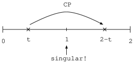
Figure 3.1: One-parameter family of chiral gauge theories

In eq. (3.64), we note that the zero-modes $\varphi_{0}^{-}$, $\varphi_{0}^{+}$ and the eigenvalues $\lambda_{j}$ are independent of $t$ (see the previous section). The change $t\to 2-t$, however, causes the exchange of $\Psi_{+}$ and $\Psi_{-}$ as shown in eq. (3.57) and thus $N\to\overline{N}$, where

$$\overline{N}=\cases{N_{-}&for $t>1$,\cr N_{+}&for $t<1$.\cr}$$ (3.77)

Thus, we immediately have

$$Z_{\rm F}[U^{\rm CP},-W^{-1}\overline{\eta}^{T},\eta^{T}W;t]$$

$$=e^{i\theta[U;2-t]}\left({\Lambda\over a}\right)^{\overline{N}}\prod^{n_{-}}\left[a^{4}\sum_{x}\overline{\eta}(x)\varphi_{0}^{-}(x)\right]\prod^{n_{+}}\left[a^{4}\sum_{x}\varphi_{0}^{+\dagger}(x)\eta(x)\right]\prod_{\lambda_{j}>0\atop\lambda_{j}\neq\Lambda}\left({\lambda_{j}\over a}\right)$$

$$\qquad\qquad\qquad\qquad\times\exp\left[a^{8}\sum_{x,y}\overline{\eta}(x)G^{(2-t)}(x,y)\eta(y)\right],$$ (3.78)

for the generating functional.

3.3.2 CP property of the measure term

To derive CP transformation law of the fermion generating functional, we must investigate the relation between the phase factors, $e^{\theta[U;t]}$ and $e^{\theta[U;2-t]}$. Since their variation under an infinitesimal variation of the link variable is described with the measure terms (3.48), we examine the CP properties of the measure terms. We first calculate the measure terms for the auxiliary basis ${\cal L}_{\xi}^{\{w,\overline{w}\}}$ and then discuss their CP properties.

Measure term for the auxiliary basis

Here, let us consider the measure term  (3.49) for the auxiliary basis. Namely,

$${\cal L}_{\xi}^{\{w,\overline{w}\}}[U;t]=i\sum_{j}(w_{j},\delta_{\xi}w_{j})+i\sum_{k}(\delta_{\xi}\overline{w}_{k}^{\dagger},\overline{w}_{k}^{\dagger}).$$ (3.79)

Noting $H^{2}w_{j}=\lambda_{j}^{2}w_{j}$ and thus

$$\delta_{\xi}\lambda_{j}^{2}=(w_{j},\delta_{\xi}H^{2}w_{j}),$$ (3.80)

we have from eq. (3.58),

$$(\delta_{\xi}\overline{w}_{j}^{\dagger},\overline{w}_{j}^{\dagger})=-{1\over 2\lambda_{j}^{2}}(w_{j},[H,\delta_{\xi}H]w_{j})+(\delta_{\xi}w_{j},w_{j}).$$ (3.81)

Taking the contribution of zero-modes into account, we thus have

$${\cal L}_{\xi}^{\{w,\overline{w}\}}[U;t]=i\sum^{n_{-}}(\varphi_{0}^{-},\delta_{\xi}\varphi_{0}^{-})+i\sum^{n_{+}}(\delta_{\xi}\varphi_{0}^{+},\varphi_{0}^{+})-{i\over 2}\sum_{\lambda_{j}>0}(\varphi_{j}^{-},[H^{-1},\delta_{\xi}H]\varphi_{j}^{-}).$$ (3.82)

The last term may be written in a basis independent way

$$-{i\over 2}\mathop{\rm Tr}\nolimits^{\prime}[H^{-1},\delta_{\xi}H]P_{-}^{(t)} = {i\over 4}\mathop{\rm Tr}\nolimits^{\prime}(H^{-1}\delta_{\xi}H\gamma_{5}^{(t)}-\delta_{\xi}HH^{-1}\gamma_{5}^{(t)})$$ (3.83)

$$= {i\over 4}\mathop{\rm Tr}\nolimits^{\prime}\delta_{\xi}H(\gamma_{5}^{(t)}+\gamma_{5}^{(2-t)})H^{-1},$$

where $\mathop{\rm Tr}\nolimits^{\prime}$ denotes the trace over the subspace of non-zero modes of the hermitian operator $H$. In deriving the last line, we have used the relation $H^{-1}\gamma_{5}^{(t)}=-\gamma_{5}^{(2-t)}H^{-1}$ being valid in this subspace. Noting $H^{-1}\gamma_{5}\gamma_{5}\delta_{\xi}H=D^{-1}\delta_{\xi}D$, we have

$${\cal L}_{\xi}^{\{w,\overline{w}\}}[U;t]=i\sum^{n_{-}}(\varphi_{0}^{-},\delta_{\xi}\varphi_{0}^{-})+i\sum^{n_{+}}(\delta_{\xi}\varphi_{0}^{+},\varphi_{0}^{+})+{i\over 4}\mathop{\rm Tr}\nolimits^{\prime}\delta_{\xi}D(\gamma_{5}^{(t)}+\gamma_{5}^{(2-t)})D^{-1}.$$ (3.84)

This expression shows that the auxiliary basis $w_{j}$ and $\overline{w}_{k}$ cannot be a physically sensible one (namely, we cannot take them as ideal basis $\{v,\overline{v}\}=\{w,\overline{w}\}$) because the measure term is non-local, containing the propagator $D^{-1}$. In fact, we see that $i{\cal L}_{\xi}^{\{w,\overline{w}\}}$ is identical to (a variation of) the main part of the imaginary part of the fermion effective action (2.47), when there are no zero-modes. Consequently, this basis when identified as $\{v,\overline{v}\}=\{w,\overline{w}\}$ modifies the physical contents of the theory, eliminating the imaginary part. This explains why the generating functional with this basis is gauge invariant, even if the fermion multiplet is not anomaly-free. Nevertheless, this basis is convenient as an intermediate tool as one can work out all the quantities.

CP properties of ${\cal L}_{\xi}^{\{w,\overline{w}\}}$ and ${\cal L}_{\xi}^{\{v,\overline{v}\}}$

From (3.84), we can see easily that the measure terms for the auxiliary basis ${\cal L}_{\xi}^{\{w,\overline{w}\}}$ is invariant under $t\to 2-t$:

$${\cal L}_{\xi}^{\{w,\overline{w}\}}[U;2-t]={\cal L}_{\xi}^{\{w,\overline{w}\}}[U;t].$$ (3.85)

Moreover, in the previous chapter, we have observed that the requirements for the ideal measure term are given by eqs. (2.51) and (LABEL:integral). The remarkable fact is that these conditions are invariant under $t\to 2-t$. Thus, if we have an ideal measure term ${\cal L}_{\xi}[U;t]$ which works for $U$ with respect to $\gamma_{5}^{(t)}$, then we may use the same measure term for $U$ with respect to $\gamma_{5}^{(2-t)}$. Therefore, we may set without loss of generality

$${\cal L}_{\xi}^{\{v,\overline{v}\}}[U;2-t]={\cal L}_{\xi}^{\{v,\overline{v}\}}[U;t].$$ (3.86)

This equality can be interpreted in a more physically transparent language; this is equivalent to the CP invariance of the measure term. To see this, let us recall that basis vectors for $U^{\rm CP}$ with respect to $\gamma_{5}^{(t)}$ [which is specified by eq. (3.70)] and basis vectors for $U$ with respect to $\gamma_{5}^{(2-t)}$ [which is specified by eq. (3.74)] can be related as eq. (3.73). This particular choice of bases, which may always be made, leads to

$${\cal L}_{\xi}[U^{\rm CP};t]={\cal L}_{\xi}[U;2-t],$$ (3.87)

and thus eq. (3.86) implies

$${\cal L}_{\xi}[U^{\rm CP};t]={\cal L}_{\xi}[U;t].$$ (3.88)

In fact, it is physically natural to take basis vectors such that the relation (3.88) holds. In the continuum theory, the action of the Weyl fermion is CP invariant and the imaginary part of the effective action is too (it is independent of the regularization chosen and is given by the so-called $\eta$-invariant [64]). This property is shared with our lattice transcription (2.47), as one can verify from CP transformation law of various operators. If the measure term is not invariant under CP, it then produces another unphysical source of CP breaking as eq. (2.44) shows. In other words, the requirement (3.88) eliminates an unnecessary CP violation which may result from a wrong choice of the fermion measure (which might be called “fake CP anomaly”). Fortunately, it is always possible to construct the CP invariant ideal measure term by the average over CP [25, 30]:

$${\cal L}_{\xi}^{\{v,\overline{v}\}}[U;t]=a^{4}\sum_{x}\xi_{\mu}^{a}(x)j_{\mu}^{a}(x)[U;t]$$

$$\to{1\over 2}\biggl{[}a^{4}\sum_{x}\xi_{\mu}^{a}(x)j_{\mu}^{a}(x)[U;t]+a^{4}\sum_{x}\xi_{\mu}^{{\rm CP}a}(x)j_{\mu}^{a}(x)[U^{\rm CP};t]\biggr{]}.$$ (3.91)

This average is possible even if $U$ and $U^{\rm CP}$ belong to different topological sectors $M$ and $M^{\rm CP}$, because the CP operation defines a differentiable one-to-one onto-mapping from $M$ to $M^{\rm CP}$. Then CP invariance of the measure term is ensured and this is equivalent to eq. (3.86), and vice versa.

From these analysis, we have

$$\delta_{\xi}\theta[U^{CP};t] = \delta_{\xi}\theta[U;2-t]$$ (3.92)

$$= -{\cal L}_{\xi}^{\{v,\overline{v}\}}[U;2-t]+{\cal L}_{\xi}^{\{w,\overline{w}\}}[U;2-t]$$

$$= \delta_{\xi}\theta[U;t],$$

and, as result,

$$\delta_{\xi}(\theta[U;2-t]-\theta[U;t])=0.$$ (3.93)

Therefore the difference, $\theta[U;2-t]-\theta[U;t]$, if it exists, is a constant:

$$\theta[U;2-t]=\theta[U;t]+\theta_{M},$$ (3.94)

where the constant $\theta_{M}$ is assigned for each topological sector $M$, $U\in M$.

3.3.3 CP transformation law of the fermion generating functional

From the above analysis, we have

$$Z_{\rm F}[U^{\rm CP},-W^{-1}\overline{\eta}^{T},\eta^{T}W;t]$$

$$=e^{i\theta_{M}}\left({\Lambda\over a}\right)^{\overline{N}-N}{\exp\left[a^{8}\sum_{x,y}\overline{\eta}(x)G^{(2-t)}(x,y)\eta(y)\right]\over\exp\left[a^{8}\sum_{x,y}\overline{\eta}(x)G^{(t)}(x,y)\eta(y)\right]}Z_{\rm F}[U,\eta,\overline{\eta};t].$$

(3.95)

In particular, in the vacuum sector which contains the trivial configuration $U_{\mu 0}(x)=1$, $U_{0}^{\rm CP}=U_{0}$ and thus one has $\theta_{M}=0$ (recall that the phase depends only on the link variable).

From eq. (3.95), we see that the CP breaking in this formulation appears in three places: (I) Difference in the overall constant phase $\theta_{M}$. (II) Difference in the overall coefficient $(\Lambda/a)^{\overline{N}-N}$ (III) Difference in the propagator, $G^{(t)}$ and $G^{(2-t)}$. We discuss their implications in this order:

(I) The constant phase $\theta_{M}$ may be absorbed into a redefinition of the phase factor $\vartheta_{M}$ in eq. (2.39) as

$$\vartheta_{M}\to\vartheta_{M}+{1\over 2}\theta_{M},\qquad\vartheta_{M^{\rm CP}}\to\vartheta_{M^{\rm CP}}-{1\over 2}\theta_{M}.$$ (3.96)

Then the overall phases in $Z_{\rm F}[U]$ and $Z_{\rm F}[U^{\rm CP}]$ become identical (no “CP anomaly” from the path integral measure) and the discussion of CP violation is reduced to how one should choose the “topological phase” $\vartheta_{M}$; this is a problem analogous to the strong CP problem in continuum theory.

(II) The breaking $(\Lambda/a)^{\overline{N}-N}$ can also be absorbed into the topological weight ${\cal N}_{M}$ in  eq. (2.39). Namely, we may redefine

$${\cal N}_{M}\to{\cal N}_{M}\left({\Lambda\over a}\right)^{(-N+\overline{N})/2},\qquad{\cal N}_{M^{\rm CP}}\to{\cal N}_{M^{\rm CP}}\left({\Lambda\over a}\right)^{(N-\overline{N})/2}.$$ (3.97)

This redefinition is consistent because the roles of $N$ and $\overline{N}$ are exchanged under $U\leftrightarrow U^{\rm CP}$. Note that

$$-N+\overline{N}=\cases{n_{+}-n_{-},&for $t>1$,\cr n_{-}-n_{+},&for $t<1$,\cr}$$ (3.98)

due to the chirality sum rule [57, 58]. (The index $n_{+}-n_{-}$ does not depend on $f(H^{2})$, see Appendix B.) The simplest CP invariant choice is then ${\cal N}_{M}=1$ for all topological sectors. However, whether this simplest choice is consistent with other physical requirements, such as the cluster decomposition, is another question which we do not discuss in this thesis. Interestingly, this simplest CP invariant choice is also suggested  [31] by a matching with the “Majorana formulation”.

(III) It seems impossible to remedy the breaking $G^{(2-t)}\neq G^{(t)}$ in the propagator. Note that the propagator is independent of the choice of the basis vectors or the path integral measure. For the symmetric choice $t=1$, $\gamma_{5}^{(1)}=\Gamma_{5}/\sqrt{\Gamma_{5}^{2}}$ is plagued with the singularity due to zero-modes of $\Gamma_{5}$, whose inevitable presence has been proven under rather mild assumptions as has been discussed before. However, observe that the CP breaking for $t\neq 1$ is quite modest. For example, when there are no zero-modes,

$$G^{(2-t)}=P_{-}^{(2-t)}{1\over D}\overline{P}_{+}^{(2-t)}=G^{(t)}+{a(1-t)f(H^{2})\over\sqrt{1+t(t-2)H^{2}f^{2}(H^{2})}}\gamma_{5},$$ (3.99)

thus the breaking term is local. In particular, for the conventional choice, $t=2$ and $f(H^{2})=1$,

$$G^{(2-t)}(x,y)=G^{(t)}(x,y)-a\gamma_{5}{1\over a^{4}}\delta_{x,y},$$ (3.100)

and the breaking appears as an (ultra-local) contact term, as we have noted in Subsec. 3.1.2. It is thus expected that this breaking is safely removed in a suitable continuum limit in the case of pure chiral gauge theory. However, there appear additional complications when the Yukawa coupling is included and the Higgs field acquires the expectation value; this issue will be discussed in the following section.

In summary, the inherent CP violation in this framework emerges only in the fermion propagator which is connected to external sources in the case of pure chiral gauge theory. This implies that diagrams with external fermion lines or with a fermion composite operator would behave differently from the naively expected one under CP, but the vacuum polarization, for example, respects CP. As for other possible sources of CP violation in relative topological weight factors, the same problem appears in continuum theory also and it is not particular to the present formulation of lattice chiral gauge theory.

3.4 CP breaking in lattice chiral gauge theories with Yukawa couplings

It is straightforward to add the Yukawa coupling to the present formulation. By introducing the right-handed Weyl fermion and the Higgs field, we set

$$S_{\rm F} = a^{4}\sum_{x}[\overline{\psi}_{L}(x)D\psi_{L}(x)+\overline{\psi}_{R}(x)D^{\prime}\psi_{R}(x)$$

$$\qquad\quad+\overline{\psi}_{L}(x)\phi(x)\psi_{R}(x)+\overline{\psi}_{R}(x)\phi^{\dagger}(x)\psi_{L}(x)$$

$$\qquad\qquad-\overline{\psi}_{L}(x)\eta_{L}(x)-\overline{\eta}_{L}(x)\psi_{L}(x)-\overline{\psi}_{R}(x)\eta_{R}(x)-\overline{\eta}_{R}(x)\psi_{R}(x)],$$

where

$$P_{-}^{(t)}\psi_{L}=\psi_{L},\qquad\overline{\psi}_{L}\overline{P}_{+}^{(t)}=\overline{\psi}_{L},$$

$$P_{+}^{\prime(t)}\psi_{R}=\psi_{R},\qquad\overline{\psi}_{R}\overline{P}_{-}^{\prime(t)}=\overline{\psi}_{R}.$$ (3.102)

We assume that the left-handed fermion $\psi_{L}(x)$ belongs to the representation $R_{L}$ of the gauge group and the right-handed fermion $\psi_{R}(x)$ belongs to $R_{R}$ (the Higgs field $\phi(x)$ transforms as $R_{L}\otimes(R_{R})^{*}$). The gauge couplings in the Dirac operator $D$ ($D^{\prime}$), and correspondingly in $P_{-}^{(t)}$ and $\overline{P}_{+}^{(t)}$ ($P_{+}^{\prime(t)}$ and $\overline{P}_{-}^{\prime(t)}$), are thus defined with respect to the representation $R_{L}$ ($R_{R}$).

From now, we assume a perturbative treatment of the Higgs coupling. Then we note the relation

$$Z_{\rm F}[U,\phi,\eta_{L},\overline{\eta}_{L},\eta_{R},\overline{\eta}_{R};t]=\int{\rm D}[\psi]{\rm D}[\overline{\psi}]\,e^{-S_{\rm F}}$$

$$=\exp\biggl{\{}a^{-4}\sum_{x}\biggl{[}{\partial\over\partial\eta_{L}(x)}\overline{P}_{+}^{(t)}\phi(x)P_{+}^{\prime(t)}{\partial\over\partial\overline{\eta}_{R}(x)}$$

$$\qquad\qquad\qquad\qquad+{\partial\over\partial\eta_{R}(x)}\overline{P}_{-}^{\prime(t)}\phi^{\dagger}(x)P_{-}^{(t)}{\partial\over\partial\overline{\eta}_{L}(x)}\biggr{]}\biggr{\}}$$

$$\qquad\qquad\qquad\qquad\qquad\qquad\qquad\qquad\qquad\qquad\times Z_{\rm F}[U,0,\eta_{L},\overline{\eta}_{L},\eta_{R},\overline{\eta}_{R};t],$$

(3.103)

because the fermion integration measure refers to neither source fields nor the Higgs field. The generating functional without the Yukawa coupling can be analyzed as before, and we have

$$Z_{\rm F}[U,0,\eta_{L},\overline{\eta}_{L},\eta_{R},\overline{\eta}_{R};t]$$

$$=e^{i\theta[U;t]}\left({\Lambda\over a}\right)^{N}\prod^{n_{-}}\left[a^{4}\sum_{x}\overline{\eta}_{L}(x)\varphi_{0}^{-}(x)\right]\prod^{n_{+}}\left[a^{4}\sum_{x}\varphi_{0}^{+\dagger}(x)\eta_{L}(x)\right]\prod_{\lambda_{j}>0\atop\lambda_{j}\neq\Lambda}\left({\lambda_{j}\over a}\right)$$

$$\qquad\qquad\qquad\qquad\times\exp\left[a^{8}\sum_{x,y}\overline{\eta}_{L}(x)G^{(t)}(x,y)\eta_{L}(y)\right]$$

$$\qquad\qquad\times\left({\Lambda\over a}\right)^{\overline{N}^{\prime}}\prod^{n_{+}^{\prime}}\left[a^{4}\sum_{x}\overline{\eta}_{R}(x)\varphi_{0}^{\prime+}(x)\right]\prod^{n_{-}^{\prime}}\left[a^{4}\sum_{x}\varphi_{0}^{\prime-\dagger}(x)\eta_{R}(x)\right]$$

$$\qquad\qquad\qquad\times\prod_{\lambda_{j}^{\prime}>0\atop\lambda_{j}^{\prime}\neq\Lambda}\left({\lambda_{j}^{\prime}\over a}\right)\,\exp\left[a^{8}\sum_{x,y}\overline{\eta}_{R}(x)G^{\prime(t)}(x,y)\eta_{R}(y)\right],$$ (3.104)

as a product of left-handed and right-handed contributions. In this expression, all quantities with the prime (^′) are defined with respect to $H^{\prime}=a\gamma_{5}D^{\prime}$ and

$$D^{\prime}G^{\prime(t)}(x,y)=\overline{P}_{-}^{\prime(t)}(x,y)-\sum^{n_{-}^{\prime}}\varphi_{0}^{\prime-}(x)\varphi_{0}^{\prime-\dagger}(y).$$ (3.105)

By repeating the same arguments as before for $Z_{\rm F}[U,0,\eta_{L},\overline{\eta}_{L},\eta_{R},\overline{\eta}_{R};t]$ we finally have, corresponding to eq. (3.95),

$$Z_{\rm F}[U^{\rm CP},\phi^{\dagger},-W^{-1}\overline{\eta}_{L}^{T},\eta_{L}^{T}W,-W^{-1}\overline{\eta}_{R}^{T},\eta_{R}^{T}W;t]$$

$$=e^{i\theta_{M}}\left({\Lambda\over a}\right)^{\overline{N}-N-\overline{N}^{\prime}+N^{\prime}}\exp\biggl{\{}a^{-4}\sum_{x}\biggl{[}{\partial\over\partial\eta_{L}(x)}\overline{P}_{+}^{(2-t)}\phi(x)P_{+}^{\prime(2-t)}{\partial\over\partial\overline{\eta}_{R}(x)}$$

$$\qquad\qquad\qquad\qquad\qquad\qquad+{\partial\over\partial\eta_{R}(x)}\overline{P}_{-}^{\prime(2-t)}\phi^{\dagger}(x)P_{-}^{(2-t)}{\partial\over\partial\overline{\eta}_{L}(x)}\biggr{]}\biggr{\}}$$

$$\qquad\times{\exp\biggl{\{}a^{8}\sum_{x,y}\biggl{[}\overline{\eta}_{L}(x)G^{(2-t)}(x,y)\eta_{L}(y)+\overline{\eta}_{R}(x)G^{\prime(2-t)}(x,y)\eta_{R}(y)\biggr{]}\biggr{\}}\over\exp\biggl{\{}a^{8}\sum_{x,y}\biggl{[}\overline{\eta}_{L}(x)G^{(t)}(x,y)\eta_{L}(y)+\overline{\eta}_{R}(x)G^{\prime(t)}(x,y)\eta_{R}(y)\biggr{]}\biggr{\}}}$$

$$\qquad\qquad\qquad\qquad\qquad\qquad\qquad\times Z_{\rm F}[U,0,\eta_{L},\overline{\eta}_{L},\eta_{R},\overline{\eta}_{R};t].$$ (3.108)

Thus we see that the effect of the CP breaking appears precisely in the same places as before, except for the terms consisting of Yukawa couplings connected by the propagators. However, when the Higgs field acquires the expectation value, a completely new situation arises. Setting $\phi(x)=v$, the fermion propagators read

$${\langle\psi_{L}(x)\overline{\psi}_{L}(y)\rangle_{\rm F}\over\langle 1\rangle_{\rm F}}=P_{-}^{(t)}{1\over D-v_{+}D^{\prime-1}v_{-}}\overline{P}_{+}^{(t)}(x,y),$$

$${\langle\psi_{L}(x)\overline{\psi}_{R}(y)\rangle_{\rm F}\over\langle 1\rangle_{\rm F}}=P_{-}^{(t)}{1\over v_{-}-D^{\prime}v_{+}^{-1}D}\overline{P}_{-}^{\prime(t)}(x,y),$$

$${\langle\psi_{R}(x)\overline{\psi}_{R}(y)\rangle_{\rm F}\over\langle 1\rangle_{\rm F}}=P_{+}^{\prime(t)}{1\over D^{\prime}-v_{-}D^{-1}v_{+}}\overline{P}_{-}^{\prime(t)}(x,y),$$

$${\langle\psi_{R}(x)\overline{\psi}_{L}(y)\rangle_{\rm F}\over\langle 1\rangle_{\rm F}}=P_{+}^{\prime(t)}{1\over v_{+}-Dv_{-}^{-1}D^{\prime}}\overline{P}_{+}^{(t)}(x,y),$$ (3.109)

where we have defined $v_{+}=\overline{P}_{+}^{(t)}vP_{+}^{\prime(t)}$ and $v_{-}=\overline{P}_{-}^{\prime(t)}v^{\dagger}P_{-}^{(t)}$. One thus sees that this time the change $t\to 2-t$ produces non-local differences in the propagator. For example, in $\langle\psi_{L}(x)\overline{\psi}_{R}(y)\rangle_{\rm F}/\langle 1\rangle_{\rm F}$, the difference $\overline{P}_{-}^{\prime(2-t)}-\overline{P}_{-}^{\prime(t)}\propto a(t-1)D^{\prime}\gamma_{5}f(H^{\prime 2})$ cannot cancel the denominator $v_{-}-D^{\prime}v_{+}^{-1}D$, leaving a non-local difference. Though we expect naively that this breaking, even if it is non-local, will eventually be removed in a suitable continuum limit, a more careful study is required to confirm this expectation. (If one forms the free Dirac-type propagator, the CP breaking does not appear in the propagator. This means that the coupling of chiral gauge fields induces CP breaking.)

Chapter 4 Conclusion and Discussion

In this thesis we have analyzed CP breaking in lattice chiral gauge theory, which is a result of the very definition of chirality (3.16) for the Ginsparg-Wilson operator [38]. First, we showed that this CP breaking is directly related to the basic notions of locality and absence of species doubling in the Ginsparg-Wilson operator [40]. Although the non-perturbative construction of the ideal path integral measure for non-abelian chiral gauge theories has not been established yet, we analyzed the CP transformation properties of the fermion generating functional on the basis of a working ansatz [41]. Our conclusion is that there exists no “CP anomaly” arising from the path integral measure. The breaking of CP is thus limited to the explicit breaking in the action of chiral gauge theory, and it basically appears in the fermion propagator in the formulation with Ginsparg-Wilson operators. When the Higgs field has no vacuum expectation value or in pure chiral gauge theory without the Higgs field, it emerges as an (almost)contact term. In the presence of the Higgs expectation value, however, the breaking becomes intrinsically non-local. We naively expect that these breakings in the propagator, either local or non-local, do not survive in a suitable continuum limit, though a detailed analysis is needed. One might also consider the CP invariant action with projection operators which are singular on top of the would-be species doublers in the case of free fermions or on top of topological modes in the presence of instantons, and one might hope that those singularities are not so serious in an appropriate continuum limit in some practical applications. But a more careful analysis is required to make a definite conclusion about these practical issues.

Let us now take up some topics related to both of the CP symmetry and the lattice chiral symmetry, which have not been described in this thesis.

CP breakings of weak matrix elements

In this thesis, we have considered CP breakings which appear in the fermion generating functional and have not investigated CP breakings in the expectation values of general composite operators. In this case, further complications could arise. As an example, we comment on the computation of the kaon $B$ parameter, $B_{K}$ in lattice QCD(see, for example, refs. [65, 66]). The following matrix element of the effective weak Hamiltonian is then relevant:

$$\langle\overline{K}^{0}|\,\overline{s}\gamma_{5}\Gamma_{5}\gamma_{\mu}{1-\gamma_{5}\over 2}\gamma_{5}\Gamma_{5}d\,\,\overline{s}\gamma_{5}\Gamma_{5}\gamma_{\mu}{1-\gamma_{5}\over 2}\gamma_{5}\Gamma_{5}d\,|K^{0}\rangle,$$ (4.1)

where we have adopted the $O(a)$ improved operator [67]. Since the gauge action and the Ginsparg-Wilson action in QCD are invariant under CP, its CP transformation:

$$\langle K^{0}|\,\overline{d}\gamma_{5}\Gamma_{5}\gamma_{\mu}{1-\gamma_{5}\over 2}\gamma_{5}\Gamma_{5}s\,\,\overline{d}\gamma_{5}\Gamma_{5}\gamma_{\mu}{1-\gamma_{5}\over 2}\gamma_{5}\Gamma_{5}s\,|\overline{K}^{0}\rangle.$$ (4.2)

coincides with the lattice transcription of the naive CP transformation of eq.
(4.1). This shows that the $O(a)$ improvement in ref. [67], which eliminates $O(a)$ chiral symmetry breakings (in the sense of continuum theory), maintains the desired behavior of the amplitude (4.1) under CP.

From a view point of the present analysis of CP symmetry in the lattice chiral gauge theory respecting the gauge invariance, however, the above $O(a)$ improved expression of the effective Hamiltonian, if applied to off-shell amplitudes, is not completely satisfactory. For example, one can confirm that the right-handed component of the $\overline{s}(1-\gamma_{5})/2$ quark contributes to the above weak effective Hamiltonian in eq. (4.1), if applied to off-shell Green’s functions. Although this is the order $O(a)$ effect, this breaks $\mathop{\rm SU}(2)_{L}$ gauge symmetry of electroweak interactions. This illustrates that great care need to be exercised in the analysis of lattice chiral symmetry and CP invariance, when the expectation values of general composite operators are considered.

Domain wall fermion and modified CP transformation

As a closely related formulation to Ginsparg-Wilson fermions, the domain wall fermion [5, 6, 34] [68]-[70] is well-known. In one representation of the domain wall fermion in the infinite flavor limit, the domain wall fermion becomes identical to the overlap fermion (A.34). In this case, one may expect that the conflict between CP symmetry and chiral theory naturally persists. Recently, in [71], the conflict with CP symmetry have been shown in a formulation of the domain wall fermion where the light field variables $q$ and $\bar{q}$ together with Pauli-Villars fields $Q$ and $\bar{Q}$ are utilized [68]-[70]. A modified form of lattice CP transformation motivated by the domain wall fermion has also been discussed there. For the left-handed Weyl fermion defined by the Dirac operator satisfying the general Ginsparg-Wilson relation (2.4), this CP transformation is defined by

$$\psi_{L}\to\psi_{L}^{CP}=-W^{-1}\left[\bar{\psi}_{L}\frac{1}{\gamma_{5}\Gamma_{5}(U)}\right]^{T},$$

$$\bar{\psi}_{L}\to\bar{\psi}_{L}^{CP}=\left[\gamma_{5}\Gamma_{5}(U)\psi_{L}\right]^{T}W,$$ (4.3)

where $\psi_{L}=\hat{P}_{-}\psi$ and $\bar{\psi}_{L}=\bar{\psi}\bar{P}_{+}$ at $t=2$ in (2.27). An interesting feature of this modified lattice CP transformation is that one can confirm that the chiral action with Ginsparg-Wilson operator is invariant under this CP transformation. Moreover, one can show that the Jacobian for this modified CP transformation gives unity and all CP violation effects appear in the source terms for $\psi_{L}$ and $\bar{\psi}_{L}$. As a result, this analysis is perfectly consistent with our present analysis, though this modified CP transformation is applicable to only the topologically trivial sector because of the singularities in $1/\gamma_{5}\Gamma_{5}(U)$.

Time reversal

We have not discussed the time-reversal in this thesis, which is the important discrete symmetry in chiral gauge theory. Since the time-reversal operator is referred to as an antilinear or antiunitary operator in continuum Lorentzian space-time, we have to begin with defining the time-reversal on the lattice, in other words, in the discrete Euclidean space-time. While one also expects the CPT invariance on the lattice, it is important to examine these symmetries in more detail.

For further analyses of these issues, we believe that this thesis will provide a good starting point.

Acknowledgments

In the first place I would like to thank Prof. Kazuo Fujikawa for having led me to this interesting field and for his continuous encouragements and numerous discussions and for many fruitful collaborations on this subject.

I am also grateful to Prof. Hiroshi Suzuki for stimulating collaborations and many creative discussions and for his kindness.

It is my pleasure to thank Prof. Atsushi Yamada, Prof. Yoshio Kikukawa and Dr. Tatsuya Noguchi for collaborations and many valuable discussions. I would also like to thank Dr. Oliver Bär, Dr. Kei-ichi Nagai, Dr. Junichi Noaki, Dr. Masataka Okamoto and Mr. Yoichi Nakayama for useful discussions.

My thanks also go to Mr. Masashi Hamanaka, Mr. Yasuaki Hikida, Dr. Tadashi Takayanagi, Mr. Tadaoki Uesugi and Mr. Taizan Watari for enlightening conversations.

I would like to thank all the members of high energy physics theory group at the University of Tokyo for their kindness.

Finally, I would like to thank Dr. Kei Morisato for her constant support and encouragement at all stages of this thesis.

Appendix A Introduction to lattice gauge theory

In this appendix we shall review the basics of lattice gauge theory concisely. First, the lattice gauge fields are introduced and the gauge action is constructed. We next point out the difficulties one encounters when putting fermions on the lattice. Finally, a recent progress in the treatment of the fermions is reviewed. The contents are restricted to those properties which are useful to understand this thesis and to theoretical issues. An excellent introduction to lattice gauge theory is provided by the reviews [72] and books [73, 74, 75].

A.1 Lattice gauge fields

Lattice gauge theory is a quantum field theory formulated on a discrete Euclidean space time. The discrete space time acts as a non-perturbative regularization scheme and enables non-perturbative studies. Since all components of momenta are limited to the Brillouin zone $[-\pi/a,\pi/a]$ at the lattice spacing $a$, there are no ultraviolet infinities.

Figure A.1: Lattice theory

Various physical quantities are calculated on the lattice and then the continuum limit is taken. When the continuum limit is taken, the bare coupling $g_{0}$ has to be tuned with the lattice spacing $a$ so that physical quantities may be finite in the limit of zero lattice spacing.

On the lattice the gauge fields are represented by link variables $U_{\mu}(x)$ on the link. The link variable is an element of the gauge group $G$, for example, $SU(N)$ or $U(1)$. The relation between $U_{\mu}(x)$ and the vector potential $A_{\mu}(x)$ is written as

$$U_{\mu}(x)=e^{iagA_{\mu}(x+a\hat{\mu}/2)}.$$ (A.1)

Under gauge transformations

$$U_{\mu}(x)\to\Lambda(x)U_{\mu}(x)\Lambda(x+a\hat{\mu})^{-1},\qquad\Lambda(x)\in\mbox{G}.$$ (A.2)

The gauge covariant variables corresponding to the field strength in continuum are plaquette variables $U_{\mu\nu}(x)$ which are the product of link variables around an elementary plaquette:

$$U_{\mu\nu}(x)=U_{\mu}(x)U_{\nu}(x+a\hat{\mu})U_{\mu}^{\dagger}(x+a\hat{\nu})U_{\nu}^{\dagger}(x).$$ (A.3)

The gauge action, which is called the Wilson action, is defined in terms of these plaquette variables as

$$S_{G}=\frac{1}{g_{0}^{2}}a^{4}\sum_{x,\mu\neq\nu}\mathop{\rm Tr}\nolimits\left(1-U_{\mu\nu}(x)\right),$$ (A.4)

with $g_{0}$ being the bare coupling. This action agrees with the continuum theory in the classical continuum limit .

A.2 Fermion doubling problem and Nielsen-Ninomiya no-go theorem

The fermion doubling is the problem that extra fermion species appear when one naively puts the fermion on the lattice. In the following, we discuss this problem. A naive massless Dirac fermion action is written as follows,

$$S_{F} = a^{4}\sum_{x}\bar{\psi}(x)D\psi(x)$$ (A.7)

$$= a^{4}\sum_{x}\bar{\psi}(x)(\partial_{\mu}+\partial_{\mu}^{*})\psi(x)$$

$$= a^{4}\sum_{x,\mu}\bar{\psi}(x)\frac{\gamma_{\mu}}{2a}\left(\psi(x+a\hat{\mu})-\psi(x-a\hat{\mu})\right),$$

which is invariant under the naive chiral symmetry

$$\psi(x) \to \psi^{\prime}(x)=\psi(x)+i\epsilon\gamma_{5}\psi(x),$$

$$\bar{\psi}(x) \to \bar{\psi}^{\prime}(x)=\bar{\psi}(x)+i\epsilon\bar{\psi}(x)\gamma_{5},$$ (A.8)

with a real infinitesimal parameter $\epsilon$ and see Appendix D for $\gamma$-matrix conventions. Then the propagator is given by

$$<\psi(x)\bar{\psi}(y)>=\int^{\pi/a}_{-\pi/a}\frac{dp^{4}}{(2\pi)^{4}}\,e^{ip(x-y)a}\frac{a}{i\sum_{\mu}\gamma_{\mu}\sin ap_{\mu}}.$$ (A.9)

We set $\tilde{p}_{\mu}=\frac{i}{a}\sin ap_{\mu}$ and see the poles of this propagator in momentum space.

Figure A.2: Plot of $\tilde{p}_{\mu}$ versus $p_{\mu}$ in the Brillouin zone

By Fig.(A.2) we easily find that $\tilde{p}_{\mu}$ has two zeros. From this, the propagator in 4 dimension has 16 massless poles. Hence the above lattice theory contains sixteen species of fermions. The excitation around $p_{\mu}=(0,0,0,0)$ is called the physical mode and 15 modes except the physical mode are called doubler modes. This is the well-known fermion doubling problem. To obtain the correct continuum limit, doubler modes must be eliminated.

A.2.1 Wilson fermion

In the lattice theory one has the freedom to add the irrelevant operator to the action and thus there are many different actions which have the same classical continuum limit. The action described above has been chosen as the simplest one. Let us now modify the action (A.7) by adding a term with a second difference operator which vanishes in the classical continuum limit [3]. Thus we have

$$S_{F}^{(W)} = a^{4}\sum_{x,\mu}\bar{\psi}(x)(\gamma_{\mu}(\partial_{\mu}+\partial_{\mu}^{*})-\frac{a}{2}r\partial_{\mu}\partial_{\mu}^{*})\psi(x)$$ (A.10)

$$= a^{4}\sum_{x,\mu}\bar{\psi}(x)\left\{\frac{\gamma_{\mu}}{2a}(\psi(x+a\hat{\mu})-\psi(x-a\hat{\mu}))\right.$$

$$\left.\qquad\qquad-\frac{r}{2a}(\psi(x+a\hat{\mu})+\psi(x-a\hat{\mu})-2\psi(x))\right\},$$

with a constant $r$ which is called the Wilson parameter. The above action has the mass term in the momentum space as follows,

$$M(p) = \frac{r}{a}\sum_{\mu}(1-\cos p_{\mu}a)$$ (A.13)

$$= \left\{\begin{array}[]{cc}0&\quad\mbox{for physical mode,}\\ C/a&\quad\mbox{for doubler modes,}\end{array}\right.$$

where $C$ is a constant which is different from each doubler mode. Thus the doubler modes get masses proportional to $r/a$ in virtue of the Wilson term. As the result the doubler modes decouple in the continuum limit when the Wilson fermion is used. It is clear, however, that the Wilson fermion action has no naive chiral symmetry (A.2) because of the Wilson term. This conflict between no doublers and that the naive chiral symmetry has been examined in detail and has been summarized in the following no-go theorem [4].

Nielsen-Ninomiya no-go theorem
Lattice Dirac operator $D$ cannot have the following properties simultaneously.

(a)

$D(x,y)$ is local.

(b)

$\tilde{D}(p)=i\gamma_{\mu}p_{\mu}+{\cal O}(ap^{2})$ for $p\ll\frac{\pi}{a}$. (the correct behaviour in the classical continuum limit)

(c)

$\tilde{D}(p)$ is invertible when $p\neq 0$ ($mod\>\frac{2\pi}{a}$). (no massless doublers)

(d)

$\left\{\gamma_{5},D\right\}=0$. (naive chiral symmetry)

where $\tilde{D}(p)$ is the Fourier transform of $D(x,y)$.

The properties (a) and (b) are important for getting the correct continuum theory in the continuum limit. Therefore this theorem suggests that one may remove the doubler modes at the expense of breaking the naive chiral symmetry and it had been considered that putting a single massless fermion on the lattice is difficult. However a recent progress allows a single massless fermion on the lattice. We discuss this in the following section.

Now that we have defined the lattice action of vector-like theory, let us construct the quantum theory by using the path integral in the remainder of this subsection. We first make the Wilson fermion action (A.10) invariant under the gauge transformations

$$\psi(x)\to\Lambda(x)\psi(x),\qquad\bar{\psi}(x)\to\bar{\psi}(x)\Lambda^{-1}(x),$$ (A.14)

where $\Lambda(x)$ is an element of the gauge group. Using the link variables $U_{\mu}(x)$, the gauge invariant fermion action is written as

$$S_{F}^{(W)} = a^{4}\sum_{x,y,\mu}\bar{\psi}(x)\left({\ooalign{\hfil/\hfil\crcr$C$}}(x,y)+B(x,y)+\frac{m_{0}}{a}\delta_{x,y}\right)\psi(y),$$ (A.18)

$$= a^{4}\sum_{x,y,\mu}\frac{1}{2a}\bar{\psi}(x)\left[\gamma_{\mu}\left(U_{\mu}(x)\psi(x+a\hat{\mu})-U_{\mu}^{\dagger}(x-a\hat{\mu})\psi(x-a\hat{\mu})\right)\right.$$

$$\left.+r\left(2\psi(x)-U_{\mu}(x)\psi(x+a\hat{\mu})-U_{\mu}^{\dagger}(x-a\hat{\mu})\psi(x-a\hat{\mu})\right)\right]$$

$$+\frac{m_{0}}{a}\bar{\psi}(x)\psi(x),$$

where ${\ooalign{\hfil/\hfil\crcr$C$}}=\gamma_{\mu}C_{\mu}$ and

$$C_{\mu}(x,y)=\frac{1}{2a}\left[\delta_{x^{\mu}+{\hat{\mu}}a,y^{\mu}}U_{\mu}(x)-\delta_{x^{\mu},y^{\mu}+{\hat{\mu}}a}U_{\mu}^{\dagger}(y)\right],$$ (A.19)

$$B(x,y)=\frac{r}{2a}\sum_{\mu}\left[2\delta_{x,y}-\delta_{x^{\mu}+{\hat{\mu}}a,y^{\mu}}U_{\mu}(x)-\delta_{x^{\mu},y^{\mu}+{\hat{\mu}}a}U_{\mu}^{\dagger}(y)\right],$$ (A.20)

with $m_{0}$ being the bare mass parameter. To construct the quantum theory, we must define the integration measure. We adopt an invariant group measure, the Haar measure, $D[U]$ as the measure of the integration over the link variables and introduce Berezin integration as the integration over fermion fields. Consequently, we obtain the path integral expression for the expectation value of ${\cal O}$:

$$\langle{\cal O}\rangle = \frac{1}{Z}\int D[U]D[\bar{\psi}]D[\psi]{\cal O}\>e^{-S},$$ (A.21)

$$Z=\int D[U]D[\bar{\psi}]D[\psi]\>e^{-S},$$

where $S=S_{G}[U]+S_{F}^{(W)}[U,\psi,\bar{\psi}]$. An arbitrary correlation function containing the fermion fields and the link variables in the above formulation can be calculated from the above path integral. Of course, when we try to treat a massless fermions, we need a fine tuning of the parameter $m_{0}$ to keep the fermion massless in the continuum limit because of the breaking of chiral symmetry.

A.2.2 Chiral gauge theory with the Wilson fermion

We have just discussed the vector-like theory on the lattice. Now we consider the lattice formulation of chiral gauge theory with the Wilson fermion. In chiral gauge theory, the chiral symmetry is gauged, but the Wilson fermion action breaks chiral symmetry. This means that this formulation breaks gauge invariance and thus we suffer from the gauge degrees of freedom and must try to recover the gauge symmetry in the continuum limit. We next illustrate the above situation by an example [14]. We assume that the fermions which have colors are left-handed. The chiral fermion action with the Wilson fermion is given by

$$S_{F}=a^{4}\sum_{x,y,\mu}\bar{\psi}_{L}(x){\ooalign{\hfil/\hfil\crcr$C$}}(x,y)\psi_{L}(y)-a\left(\bar{\psi}_{R}(x)B(x,y)\psi_{L}(y)+h.c.\right),$$ (A.24)

where

$$\psi_{L}=\frac{1-\gamma_{5}}{2}\psi,\qquad\bar{\psi}_{L}=\bar{\psi}\frac{1+\gamma_{5}}{2},$$

$$\psi_{R}=\frac{1+\gamma_{5}}{2}\psi,\qquad\bar{\psi}_{R}=\bar{\psi}\frac{1-\gamma_{5}}{2},$$ (A.26)

and where $\psi_{R}$ is a gauge-neutral fermion introduced only in order to remove the doublers of the charged left-handed fermion $\psi_{L}$. After the gauge transformations $\psi_{L}(x)\to\Lambda(x)$ and $U_{\mu}(x)\to\Lambda(x)U_{\mu}(x)\Lambda(x+a\hat{\mu})$, this action becomes

$$S_{F}=a^{4}\sum_{x,y,\mu}\bar{\psi}_{L}(x){\ooalign{\hfil/\hfil\crcr$C$}}(x,y)\psi_{L}(y)-a\left(\bar{\psi}_{R}(x)\Lambda(x)B(x,y)\psi_{L}(y)+h.c.\right).$$ (A.29)

We see that the gauge degrees of freedom $\Lambda(x)$ couple to the fermion because the Wilson term breaks the gauge symmetry. The dynamics of this coupling has drastic consequences for the fermion spectrum:for instance, the theory becomes vector-like in the continuum limit [76]. It is clear that we need a more clever idea if we use the Wilson fermion in the construction of lattice chiral gauge theory. In this direction, two methods have been known:one using different cutoffs for the fermions and the link variables and another using the gauge fixing to control the gauge degrees of freedom. In the latter method, abelian chiral gauge theory has been constructed in the continuum limit [77].

A.3 Massless fermion on the lattice

The first breakthrough in the attempts to put a massless fermion on the lattice may be traced to the domain wall fermion [5, 6], which was followed by the overlap formalism [8, 9] and then a remarkable identity, which first appeared in 1982 in the paper of Ginsparg and Wilson [11], was re-discovered [10, 7]. This identity is the Ginsparg-Wilson relation:

$$D\gamma_{5}+\gamma_{5}D=2aD\gamma_{5}D.$$ (A.31)

This relation avoids the Nielsen-Ninomiya no-go theorem on account of the term proportional to the lattice spacing in the right-hand side. The above relation can be written, in terms of the kernel of Dirac operator, as follows,

$$D^{-1}(x.y)\gamma_{5}+\gamma_{5}D^{-1}(x,y)=2a\gamma_{5}\delta_{x,y}.$$ (A.32)

This expression means that the breaking of the naive chiral symmetry would not have the effect on the physical amplitudes. Besides this relation represents the exact lattice chiral symmetry [12]. The fermion action with the Ginsparg-Wilson Dirac operator is invariant under the following transformation:

$$\psi\rightarrow\psi^{\prime}=\psi+i\epsilon\hat{\gamma}_{5}\psi,$$

$$\bar{\psi}\rightarrow\bar{\psi}^{\prime}=\bar{\psi}+i\epsilon\bar{\psi}\gamma_{5},$$ (A.33)

where $\hat{\gamma}_{5}\equiv\gamma_{5}-2a\gamma_{5}D\quad(\hat{\gamma}_{5}^{2}=1)$. Thus it is expected that the formulation with the Ginsparg-Wilson fermion has the same properties as the continuum theory with the chiral symmetry . In general, the Ginsparg-Wilson relation, however, does not guarantee the locality of the Dirac operator and no doublers. Therefore it is important to find the Dirac operator satisfying the Ginsparg-Wilson relation with such good properties. One of such Dirac operators is the overlap Dirac operator [7], which is described explicitly as 

$$D=\frac{1}{2a}\left(1+D_{W}\frac{1}{\sqrt{D^{\dagger}_{W}D_{W}}}\right),$$ (A.34)

with $D_{W}$ is the Wilson-Dirac operator with the negative mass:

$$D_{W}(x,y)={\ooalign{\hfil/\hfil\crcr$C$}}(x,y)+B(x,y)-\frac{1}{a}m_{0}\delta_{x,y},$$ (A.37)

with (A.19). The overlap Dirac operator is gauge-covariant and also is local and smooth function of link variables when the admissibility condition [47, 48]:

$$\|1-R[U_{\mu\nu}(x)]\|<\frac{1}{6(2+\sqrt{2})},$$ (A.38)

is satisfied for all plaquette variables . The fermion propagator has the single pole for the physical mode and is free from species doublers, when we take $0<m_{0}<2$. Moreover, the axial anomaly from the fermion measure has been evaluated [53]-[56] in the continuum limit and also the perturbative properties of the lattice QCD with this Dirac operator has been discussed [79]-[82]. In addition, unitarity also has been established on the lattice in the case of free fermion by showing that a Källén-Lehmann representation of the fermion propagator has non-negative spectral density [16]. All analysis clearly show that the lattice theory with the overlap Dirac operator reproduces the properties of massless Dirac fermion in continuum theory well. The overlap Dirac operator satisfies the properties of (a), (b) and (c) in Nielsen-Ninomiya’s theorem, but, of course, doesn’t satisfy (d).

Here, let us mention the definition of locality on the lattice. As the definition of locality, we have adopted the exponential locality, which means that the kernel has exponentially decaying tails at large distances:

$$\|D(x,y)\|\leq C\,e^{-\gamma|x-y|/a},$$ (A.39)

where $\gamma$ and $C$ are constants and the norm $\|M\|$ for a matrix $M$ is defined by

$$\|M\|=\sqrt{\lambda_{max}(M^{\dagger}M)},$$ (A.40)

where $\lambda_{max}$ is maximal eigenvalues of $M$. The overlap Dirac operator (A.34) is an example of the Dirac operator with such a locality. From the view point of continuum limit this locality is as good as the strict locality.

A.3.1 Algebraic generalization of the Ginsparg-Wilson relation

It is important to seek alternative lattice Dirac operators, from a theoretical viewpoint, to deepen the understanding of Ginsparg-Wilson fermions. From a numerical one, one might hope to improve the properties, such as chiral symmetry and locality of Dirac operators, compared to the overlap Dirac operator and the fixed point action. While this task is challenging and difficult, a new class of lattice Dirac operators which are based on the algebraically generalized Ginsparg-Wilson relation have been proposed [42]. This general Ginsparg-Wilson relation is written as

$$\gamma_{5}D+D\gamma_{5}=2aD(a\gamma_{5}D)^{2k}\gamma_{5}D,$$ (A.41)

where $k$ stands for a non-negative integer, and $k=0$ corresponds to the ordinary Ginsparg-Wilson relation. The solution $D$ of this general Ginsparg-Wilson relation (A.41) is given by

$$D = \frac{1}{a}\gamma_{5}\left[\frac{1}{2}\gamma_{5}\left(1+D_{W}^{(2k+1)}\frac{1}{\sqrt{D^{(2k+1)\dagger}_{W}D_{W}^{(2k+1)}}}\right)\right]^{1/(2k+1)},$$ (A.42)

where

$$D_{W}^{(2k+1)} = i({\ooalign{\hfil/\hfil\crcr$C$}})^{2k+1}+(B)^{2k+1}-\left(\frac{m_{0}}{a}\right)^{2k+1},$$ (A.45)

with $C_{\mu}$ and $B$ in (A.19). In this class of lattice Dirac operators, $k=0$ corresponds to the overlap Dirac operator. When the parameter $m_{0}$ is chosen as $0<m_{0}<2r$ in these operators, the free propagators have a single massless pole and no doublers. The locality properties have been confirmed strictly in the case of the free operator [44]. In addition, it has been shown that the formulation with these operators gives the correct chiral and Weyl anomalies [43, 45] and thus the topological properties of these operators are identical to those of the standard overlap Dirac operator.

A salient feature of Dirac operators corresponding to larger $k$ is that the chiral symmetry(in the sense of continuum) breaking term becomes more irrelevant in the sense of Wilsonian renormalization group. For the operators (A.42), in the near continuum configurations, we see the behavior as follows

$$D \simeq i{\ooalign{\hfil/\hfil\crcr$D$}}+a^{2k+1}(\gamma_{5}i{\ooalign{\hfil/\hfil\crcr$D$}})^{2k+2},$$ (A.51)

where ${\ooalign{\hfil/\hfil\crcr$D$}}=\gamma_{\mu}(\partial_{\mu}+igA_{\mu})$. The first terms in this expression stands for the leading term in chiral symmetric terms, and the second term stands for the leading term in chiral symmetry breaking terms. This shows that one can improve the chiral symmetry for larger $k$. As another manifestation of this property, the spectrum of the operators with $k\geq 1$ is closer to that of the continuum operator in the sense that the small eigenvalues of $D$ accumulate along the imaginary axis (which is a result of taking a $2k+1$-th root) [83], compared to the overlap Dirac operator for which the eigenvalues of $D$ draw a perfect circle in the complex eigenvalue plane. However, the locality property becomes worse for larger $k$. To understand the properties of these operators better, a detailed numerical study of locality and chiral symmetry has to be performed for larger $k$.

We can thus formulate the lattice theory with Ginsparg-Wilson fermions
(either by the conventional one or its generalization) at the quantum level, using the same fermion measure as discussed in Subsec.A.2.1. In this formulation, we need no fine-tuning to keep the fermion massless, while we have needed in the formulation with Wilson fermions. The formulation with Ginsparg-Wilson fermions has enabled to calculate the physical quantities that the chiral symmetry is important, for example, the $CP$-violation parameter in the Standard Model $\epsilon^{\prime}/\epsilon$ and has opened the possibility to construct the chiral gauge theory on the lattice with exact gauge invariance. See Chapter. 2.

Appendix B Eigenvalue problem of $H$

In this Appendix we consider the following eigenvalue problem for the operator $H$ satisfying the general Ginsparg-Wilson relation (2.4):

$$H\varphi_{n}(x)=\lambda_{n}\varphi_{n}(x),\qquad(\varphi_{n},\varphi_{m})=\delta_{nm}.$$ (B.1)

We note

$$H\Gamma_{5}\varphi_{n}(x)=-\Gamma_{5}H\varphi_{n}(x)=-\lambda_{n}\Gamma_{5}\varphi_{n}(x),$$ (B.2)

and

$$(\Gamma_{5}\varphi_{n},\Gamma_{5}\varphi_{m})=[1-\lambda_{n}^{2}f^{2}(\lambda_{n}^{2})]\delta_{nm}.$$ (B.3)

These relations show that eigenfunctions with $\lambda_{n}\neq 0$ (when $\lambda_{n}=0$, $\varphi_{0}(x)$ and $\Gamma_{5}\varphi_{0}(x)$ are not necessarily linear-independent) and $\lambda_{n}f(\lambda_{n}^{2})\neq\pm 1$ come in pairs as $\lambda_{n}$ and $-\lambda_{n}$.

We can thus classify eigenfunctions in eq. (B.1) as follows:

(i) $\lambda_{n}=0$ ($H\varphi_{0}(x)=0$). For this

$$H{1\pm\gamma_{5}\over 2}\varphi_{0}(x)=H{1\pm\Gamma_{5}\over 2}\varphi_{0}(x)={1\mp\Gamma_{5}\over 2}H\varphi_{0}(x)=0,$$ (B.4)

so we may impose the chirality on $\varphi_{0}(x)$ as

$$\gamma_{5}\varphi_{0}^{\pm}(x)=\Gamma_{5}\varphi_{0}^{\pm}(x)=\pm\varphi_{0}^{\pm}(x).$$ (B.5)

We denote the number of $\varphi_{0}^{+}(x)$ ($\varphi_{0}^{-}(x)$) as $n_{+}$ ($n_{-}$).

(ii) $\lambda_{n}\neq 0$ and $\lambda_{n}f(\lambda_{n}^{2})\neq\pm 1$. As shown above,

$$H\varphi_{n}(x)=\lambda_{n}\varphi_{n}(x),\qquad H\widetilde{\varphi}_{n}(x)=-\lambda_{n}\widetilde{\varphi}_{n}(x),$$ (B.6)

where

$$\widetilde{\varphi}_{n}(x)={1\over\sqrt{1-\lambda_{n}^{2}f^{2}(\lambda_{n}^{2})}}\Gamma_{5}\varphi_{n}(x).$$ (B.7)

We have

$$\Gamma_{5}\varphi_{n}(x)=\sqrt{1-\lambda_{n}^{2}f^{2}(\lambda_{n}^{2})}\widetilde{\varphi}_{n}(x),\qquad\Gamma_{5}\widetilde{\varphi}_{n}(x)=\sqrt{1-\lambda_{n}^{2}f^{2}(\lambda_{n}^{2})}\varphi_{n}(x),$$ (B.8)

and

$$\gamma_{5}\pmatrix{\varphi_{n}\cr\widetilde{\varphi}_{n}\cr}=\pmatrix{\lambda_{n}f(\lambda_{n}^{2})&\sqrt{1-\lambda_{n}^{2}f^{2}(\lambda_{n}^{2})}\cr\sqrt{1-\lambda_{n}^{2}f^{2}(\lambda_{n}^{2})}&-\lambda_{n}f(\lambda_{n}^{2})\cr}\pmatrix{\varphi_{n}\cr\widetilde{\varphi}_{n}\cr}.$$ (B.9)

(iii) $\lambda_{n}f(\lambda_{n}^{2})=\pm 1$, or

$$H\Psi_{\pm}(x)=\pm\Lambda\Psi_{\pm}(x),\qquad\Lambda f(\Lambda^{2})=1.$$ (B.10)

We see

$$\Gamma_{5}\Psi_{\pm}(x)=0,$$ (B.11)

and

$$\gamma_{5}\Psi_{\pm}(x)=\pm\Lambda f(\Lambda^{2})\Psi_{\pm}(x)=\pm\Psi_{\pm}(x).$$ (B.12)

We denote the number of $\Psi_{+}(x)$ ($\Psi_{-}(x)$) as $N_{+}$ ($N_{-}$). As a application of the above relations, we have

$$\mathop{\rm Tr}\nolimits\gamma_{5}=n_{+}-n_{-}+N_{+}-N_{-}.$$ (B.13)

If we further note $\mathop{\rm Tr}\nolimits\gamma_{5}=0$ on the lattice, we have the chirality sum rule [57, 58]

$$n_{+}-n_{-}+N_{+}-N_{-}=0.$$ (B.14)

Appendix C Some computations

eqs. (2.63)

We now prove the left side of eqs. (2.63). The right-side one is shown by the same procedure. To prove the left-side equation, we first define an operator $A_{\tau}^{(t)}$ as follows

$$A_{\tau}^{(t)}=Q_{\tau}^{(t)\dagger}P_{\tau}^{(t)}Q_{\tau}^{(t)}.$$ (C.1)

Then we need to show $A_{\tau}^{(t)}=P_{0}^{(t)}$. For this purpose, we now note that for $\tau=0$,

$$A_{0}^{(t)}=P_{0}^{(t)},$$ (C.2)

on account of $Q_{0}^{(t)}=1$. When we differentiate this operator with respect to $\tau$, we have

$$\partial_{\tau}A_{\tau}^{(t)} = -Q_{\tau}^{(t)\dagger}\partial_{\tau}P_{\tau}^{(t)}P_{\tau}^{(t)}Q_{\tau}^{(t)}+Q_{\tau}^{(t)\dagger}\partial_{\tau}P_{\tau}^{(t)}Q_{\tau}^{(t)}$$ (C.3)

$$-Q_{\tau}^{(t)\dagger}P_{\tau}^{(t)}\partial_{\tau}P_{\tau}^{(t)}Q_{\tau}^{(t)}$$

$$= 0,$$

where we used the differential equation (2.62) and

$$P_{\tau}^{(t)}\partial_{\tau}P_{\tau}^{(t)}P_{\tau}^{(t)}=0.$$ (C.4)

From (C.2) and (C.3), we obtain $A_{\tau}^{(t)}=P_{0}^{(t)}$, i.e.

$$P_{\tau}^{(t)}=Q_{\tau}^{(t)}P_{0}^{(t)}Q_{\tau}^{(t)\dagger}.$$ (C.5)

eq. (2.64)

We here compute the Wilson line (2.60) with a basis $\left\{v,\bar{v}\right\}$ along a closed curve, for which $U^{1}=U^{0}$, and show that it is equal to (2.64). Now the measure term is given by

$${\cal L}_{\xi}=i\sum_{j}\left(v_{j},\partial_{\tau}v_{j}\right)+i\sum_{k}(\partial_{\tau}\overline{v}_{k}^{\dagger},\overline{v}_{k}^{\dagger}).$$ (C.6)

We assume the basis $\left\{v_{j},\bar{v}_{j}\right\}$ as $v_{j}|_{\tau=1}=v_{j}|_{\tau=0}$ and $\bar{v}_{k}^{\dagger}|_{\tau=1}=\bar{v}_{k}^{\dagger}|_{\tau=0}$ and write the basis for $U^{\tau}$ as follows

$$v_{j}=Q_{\tau}^{(t)}\sum_{l}v_{l}|_{\tau=0}(S^{-1})_{lj},$$

$$\bar{v}_{k}^{\dagger}=\gamma_{5}Q_{\tau}^{(2-t)}\gamma_{5}\sum_{m}\bar{v}_{m}^{\dagger}|_{\tau=0}(\bar{S}^{-1})_{mk}.$$ (C.7)

where $S$ is the unitary-representation matrix of $Q_{\tau}^{(t)}$ on the space of left-handed fields and $\bar{S}$ is the one of $\gamma_{5}Q_{\tau}^{(2-t)}\gamma_{5}$ on the right-handed antifields and $S|_{\tau=0}=1$ and $\bar{S}|_{\tau=0}=1$. Substituting this basis for (C.6), we have

$${\cal L}_{\xi} = -i\mathop{\rm Tr}\nolimits S^{-1}\partial_{\tau}S-i\mathop{\rm Tr}\nolimits\bar{S}\partial_{\tau}(\bar{S}^{-1})$$ (C.8)

$$= -i\left(\partial_{\tau}ln\det S+\partial_{\tau}ln\det\bar{S}^{-1}\right),$$

where we used (2.62). Then the Wilson line along all closed curves is given by

$$W = \det S|_{\tau=1}\det\nolimits^{-1}\bar{S}|_{\tau=1}$$ (C.9)

$$= \det(1-P_{-0}^{(t)}+P_{-0}^{(t)}Q_{1}^{(t)})\det\nolimits^{-1}(1-\overline{P}_{+0}^{(t)}+\overline{P}_{+0}^{(t)}\gamma_{5}Q_{1}^{(2-t)}\gamma_{5})$$

$$= \det(1-P_{-0}^{(t)}+P_{-0}^{(t)}Q_{1}^{(t)})\det\nolimits^{-1}\left\{\gamma_{5}(1-\overline{P}_{+0}^{(t)}+\overline{P}_{+0}^{(t)}\gamma_{5}Q_{1}^{(2-t)}\gamma_{5})\gamma_{5}\right\}$$

$$= \det(1-P_{-0}^{(t)}+P_{-0}^{(t)}Q_{1}^{(t)})\det\nolimits^{-1}(1-P_{+0}^{(2-t)}+P_{+0}^{(2-t)}Q_{1}^{(2-t)}),$$

where we have written the signs of the chirality explicitly and $P_{+0}^{(2-t)}=P_{+}^{(2-t)}|_{U=U^{0}}$. From the third line to the fourth line in the above equation, we have utilized eq. (2.25). Noting the following equation:

$$(1-P_{+0}^{(2-t)}+P_{+0}^{(2-t)}Q_{1}^{(2-t)})(1-P_{-0}^{(2-t)}+P_{-0}^{(2-t)}Q_{1}^{(2-t)})=Q_{1}^{(2-t)},$$

and $\det Q_{\tau}^{(t)}=1$, we have

$$\det\nolimits^{-1}(1-P_{+0}^{(2-t)}+P_{+0}^{(2-t)}Q_{1}^{(2-t)})=\det(1-P_{-0}^{(2-t)}+P_{-0}^{(2-t)}Q_{1}^{(2-t)}),$$ (C.11)

and consequently obtain eq. (2.64).

Appendix D Conventions

This Appendix summarizes the $\gamma-$matrices convention and the definitions of $C$, $P$ and $CP$ transformations. We adopt the following convention of $\gamma$-matrices:

$$\{\gamma_{\mu},\gamma_{\nu}\}=2\delta_{\mu\nu},\qquad\gamma_{\mu}^{\dagger}=\gamma_{\mu},\qquad\gamma_{5}=-\gamma_{1}\gamma_{2}\gamma_{3}\gamma_{4}=\gamma_{5}^{\dagger},$$

$$\gamma_{1}^{T}=-\gamma_{1},\qquad\gamma_{2}^{T}=\gamma_{2},\qquad\gamma_{3}^{T}=-\gamma_{3},\qquad\gamma_{4}^{T}=\gamma_{4},\qquad\gamma_{5}^{T}=\gamma_{5}.$$

The charge conjugation is defined by

$$\psi(x)\to-C^{-1}\overline{\psi}^{T}(x),\qquad\overline{\psi}(x)\to\psi^{T}(x)C,$$

$$U(x,\mu)\to U^{\rm C}(x,\mu)=U(x,\mu)^{*},$$ (D.2)

where the charge conjugation matrix $C=\gamma_{2}\gamma_{4}$ satisfies

$$C^{\dagger}C=1,\qquad C^{T}=-C,\qquad C\gamma_{\mu}C^{-1}=-\gamma_{\mu}^{T},\qquad C\gamma_{5}C^{-1}=\gamma_{5}^{T}.$$ (D.3)

Under this transformation, the kernel of Dirac operator transforms as

$$D(U^{\rm C})(x,y)=C^{-1}D(U)(x,y)^{T}C,$$ (D.4)

where the transpose operation $T$ acts not only on the matrices involved but also on the arguments as $(x,y)\to(y,x)$.

The parity transformation is defined by

$$\psi(x)\to\gamma_{4}\psi(\bar{x}),\qquad\overline{\psi}(x)\to\overline{\psi}(\bar{x})\gamma_{4},$$

$$U(x,\mu)\to U^{\rm P}(x,\mu)=\cases{U(\bar{x}-a\hat{i},i)^{-1},&for $\mu=i$,\cr U(\bar{x},4),&for $\mu=4$,\cr}$$ (D.5)

where

$$\bar{x}=(-x_{i},x_{4}),$$ (D.6)

for $x=(x_{i},x_{4})$ ($i=1$, $2$, $3$). Under this,

$$D(U^{\rm P})(x,y)=\gamma_{4}D(U)(\bar{x},\bar{y})\gamma_{4}.$$ (D.7)

Finally, we define the CP transformation as

$$\psi(x)\to-W^{-1}\overline{\psi}^{T}(\bar{x}),\qquad\overline{\psi}(x)\to\psi^{T}(\bar{x})W$$

$$U_{\mu}(x)\to U^{\rm CP}_{\mu}(x)=\cases{{U_{i}(\bar{x}-a\hat{i})^{-1}}^{*},&for $\mu=i$,\cr U_{4}(\bar{x})^{*},&for $\mu=4$,\cr}$$ (D.8)

where

$$W=\gamma_{2},\qquad W^{\dagger}W=1,$$

$$W\gamma_{\mu}W^{-1}=\cases{\gamma_{i}^{T},&for $\mu=i$,\cr-\gamma_{4}^{T},&for $\mu=4$,\cr}\qquad W\gamma_{5}W^{-1}=-\gamma_{5}^{T},$$ (D.9)

and thus CP acts on the plaquette variables $U_{\mu\nu}(x)$ as ($\varphi_{ij}(\bar{x}-a\hat{i}-a\hat{j})=U_{j}(\bar{x}-a\hat{i}-a\hat{j})^{*}U_{i}(\bar{x}-a\hat{i})^{*}$)

$$U_{ij}(x)$$

$$\to U^{\rm CP}_{ij}(x)=\varphi_{ij}(\bar{x}-a\hat{i}-a\hat{j})^{-1}U_{ij}(\bar{x}-a\hat{i}-a\hat{j})^{*}\varphi_{ij}(\bar{x}-a\hat{i}-a\hat{j}),$$

$$U_{i4}(x)\to U^{\rm CP}_{i4}(x)={U_{i}(\bar{x}-a\hat{i})^{*}}^{-1}{U_{i4}(\bar{x}-a\hat{i})^{-1}}^{*}U_{i}(\bar{x}-a\hat{i})^{*}.$$ (D.10)

Under this transformation, we have

$$D(U^{\rm CP})(x,y)=W^{-1}D(U)(\bar{x},\bar{y})^{T}W.$$ (D.11)

The CP transformation properties of various operators, which are used in this thesis, are given by

$$H(U^{CP})=-W^{-1}(\gamma_{5}H(U)\gamma_{5})^{T}W,\qquad H(U^{CP})^{2}=W^{-1}H(U)^{2}W$$

$$\Gamma_{5}(U^{CP})=-W^{-1}(\gamma_{5}\Gamma_{5}(U)\gamma_{5})^{T}W,\qquad\gamma_{5}\Gamma_{5}(U^{CP})=W^{-1}(\gamma_{5}\Gamma_{5}(U))^{T}W,$$

and

$$\gamma_{5}^{(t)}(U^{\rm CP})=-W^{-1}\overline{\gamma}_{5}^{(2-t)}(U)^{T}W,\qquad\overline{\gamma}_{5}^{(t)}(U^{\rm CP})=-W^{-1}\gamma_{5}^{(2-t)}(U)^{T}W,$$

$$P_{\pm}^{(t)}(U^{\rm CP})=W^{-1}\overline{P}_{\mp}^{(2-t)}(U)^{T}W,\qquad\overline{P}_{\pm}^{(t)}(U^{\rm CP})=W^{-1}P_{\mp}^{(2-t)}(U)^{T}W,$$

Throughout this thesis, the transpose operation and the complex conjugation of an operator are defined with respect to the corresponding kernel in position space. Strictly speaking, the coordinates $x$ in these expressions are replaced, for example, by $\bar{x}=(-x_{i},x_{4})$ under CP. We can forgo writing this explicitly, because our final expressions always involve an integration over $x$ and $\sum_{x}=\sum_{\bar{x}}$.

Bibliography

- [1] K. Wilson, Confinement of quarks, Phys. Rev. D10 (1974) 2445
- [2] For instance, Lattice 2001, Nucl. Phys. B(Proc. Suppl.) 106 (2002)
- [3] K. Wilson, Quarks and strings on a lattice, New Phenomena in Subnuclear Physics, ed, A. Zichichi (Plenum Press, New York, 1977)
- [4] N. B. Nielsen and M. Ninomiya, No go theorem for regularizing chiral fermions, Phys. Lett. B105 (1981) 219; Absence of neutrinos on a lattice.1. Proof by Homotopy theory, Nucl. Phys. B185 (1981) 20, Erratum-ibid.B 195(1982) 541
- [5] D.B. Kaplan, A method for simulating chiral fermions on the lattice, Phys. Lett. B288 (1992) 342 [hep-lat/9206013].
-
[6]
Y. Shamir,
Chiral fermions from lattice boundaries,
Nucl. Phys. B406 (1993) 90 [hep-lat/9303005];
V. Furman and Y. Shamir, Axial symmetries in lattice QCD with Kaplan fermions, Nucl. Phys. B439 (1995) 54 [hep-lat/9405004]. - [7] H. Neuberger, Exactly massless quarks on the lattice, Phys. Lett. B417 (1998) 141 [hep-lat/9707022]; More about exactly massless quarks on the lattice, Phys. Lett. B427 (1998) 353 [hep-lat/9801031].
- [8] R. Narayanan and H. Neuberger, Infinitely many regulator fields for chiral fermions, Phys. Lett. B302 (1993) 62 [hep-lat/9212019]; Chiral determinant as an overlap of two vacua, Nucl. Phys. B412 (1994) 574 [hep-lat/9307006]; Chiral fermions on the lattice, Phys. Rev. Lett. 71 (1993) 3251 [hep-lat/9308011]; A construction of lattice chiral gauge theories, Nucl. Phys. B443 (1995) 305 [hep-th/9411108].
- [9] S. Randjbar-Daemi and J. Strathdee, On the overlap formulation of chiral gauge theory, Phys. Lett. B348 (1995) 543 [hep-th/9412165]; Chiral fermions on the lattice, Nucl. Phys. B443 (1995) 386 [hep-lat/9501027]; On the overlap prescription for lattice regularization of chiral fermions, Nucl. Phys. B466 (1996) 335 [hep-th/9512112]; Consistent and covariant anomalies in the overlap formulation of chiral gauge theories, Phys. Lett. B402 (1997) 134 [hep-th/9703092].
- [10] P. Hasenfratz, Prospects for perfect actions, Nucl. Phys. B(Proc. Suppl.) 63 (1998) 53 [hep-lat/9709110]; The theoretical background and properties of perfect actions, Lecture note prepared for Advanced Summer School on Nonperturvative Quantum Field Physics, Peniscola, Spain, 1997, hep-lat/9803027.
- [11] P. H. Ginsparg and K. G. Wilson, A remnant of chiral symmetry on the lattice, Phys. Rev. D25 (1982) 2649.
- [12] M. Lüscher, Exact chiral symmetry on the lattice and the Ginsparg-Wilson relation Phys. Lett. B428 (1998) 342 [hep-lat/9802011].
- [13] F. Niedermayer, Exact chiral symmetry, topological charge and related topics, Nucl. Phys. B(Proc. Suppl.) 73 (1999) 105 [hep-lat/9810026].
- [14] M. Golterman, Lattice chiral gauge theories, Nucl. Phys. B(Proc. Suppl.) 94 (2001) 189 [hep-lat/0011027] and references therein.
- [15] H. Neuberger, Exact chiral symmetry on the lattice, Ann. Rev. Nucl. Part. Sci. 51 (2001) 23 [hep-lat/0101006].
- [16] M. Lüscher, Chiral gauge theories revisited, Lectures given at the international school of subnuclear physics, Erice 2000, hep-th/0102028.
- [17] Y. Kikukawa, Analytic progress on exact lattice chiral symmetry, Nucl. Phys. B(Proc. Suppl.) 106 (2002) 71 [hep-lat/0111035].
- [18] J. I. Noaki et al. [CP-PACS Collaboration], Calculation of non-leptonic kaon decay amplitudes from K matrix elements in quenched domain-wall QCD, hep-lat/0108013.
- [19] T. Blum et al. [RBC Collaboration], Kaon matrix elements and CP-violation from quenched lattice QCD. I: The 3-flavor case, hep-lat/0110075.
- [20] N. Ishizuka, K decay amplitude on the lattice, hep-lat/0209108 and references therein.
-
[21]
S. Weinberg,
The quantum theory of fields I, II
(Cambridge university press, 1995, 1996);
M. Peskin and D. Schroeder, An introduction to quantum field theory (Addison-Wesley, 1995) - [22] L. Alvarez-Gaumé, An introduction to anomalies, Fundamental problems of gauge field theory, eds, G. Velo and A. S. Wightman (Plenum Press, New York, 1986).
- [23] E. Witten, An SU(2) Anomaly, Phys. Lett. B 117 (1982) 324.
- [24] S. Elitzur and V. P. Nair, Nonperturbative Anomalies In Higher Dimensions, Nucl. Phys. B 243 (1984) 205.
- [25] M. Lüscher, Abelian chiral gauge theories on the lattice with exact gauge invariance, Nucl. Phys. B549 (1999) 295 [hep-lat/9811032].
- [26] H. Suzuki, Gauge invariant effective action in abelian chiral gauge theory on the lattice, Prog. Theor. Phys. 101 (1999) 1147 [hep-lat/9901012].
- [27] M. Lüscher, Weyl fermions on the lattice and the non-abelian gauge anomaly, Nucl. Phys. B568 (2000) 162 [hep-lat/9904009].
-
[28]
H. Suzuki,
Anomaly cancellation condition in lattice gauge theory,
Nucl. Phys. B585 (2000) 471 [hep-lat/0002009];
H. Igarashi, K. Okuyama and H. Suzuki, Errata and addenda to “Anomaly cancellation condition in lattice gauge theory”, hep-lat/0012018. - [29] Y. Kikukawa and Y. Nakayama, Gauge anomaly cancellation in electroweak theory on the lattice, Nucl. Phys. B597 (2001) 519 [hep-lat/0005015].
- [30] M. Lüscher, Lattice regularization of chiral gauge theories to all orders of perturbation theory, J. High Energy Phys.06 (2000) 028 [hep-lat/0006014].
- [31] H. Suzuki, Real representation in chiral gauge theories on the lattice, J. High Energy Phys.10 (2000) 039 [hep-lat/0009036].
- [32] O. Bar and I. Campos, Global anomalies in chiral gauge theories on the lattice, Nucl. Phys. B 581 (2000) 499, [hep-lat/0001025].
- [33] O. Bar, On Witten’s global anomaly for higher SU(2) representations, hep-lat/0209098.
- [34] Y. Kikukawa, Domain wall fermion and chiral gauge theories on the lattice with the exact gauge invariance, Phys. Rev. D65 (2002) 074504, [hep-lat/0105032].
- [35] H. Neuberger, Geometrical aspects of chiral anomalies in the overlap, Phys. Rev. D59 (1999) 085006, [hep-lat/9802033].
- [36] H. Neuberger, Noncompact chiral U(1) gauge theories on the lattice, Phys. Rev. D63 (2001) 014503, [hep-lat/0002032].
- [37] H. Neuberger, Witten’s SU(2) anomaly on the lattice, Phys. Lett. B437 (1998) 117, [hep-lat/9805027]
- [38] P. Hasenfratz, Lattice 2001: Reflections, Nucl. Phys. B(Proc. Suppl.) 106 (2002) 159 [hep-lat/0111023] and references therein.
- [39] R. Narayanan, Ginsparg-Wilson relation and the overlap formula, Phys. Rev. D58 (1998) 097501 [hep-lat/9802018].
- [40] K. Fujikawa, M. Ishibashi and H. Suzuki, Ginsparg-Wilson operators and a no-go theorem, Phys. Lett. B538 (2002) 197 [hep-lat/0202017].
- [41] K. Fujikawa, M. Ishibashi and H. Suzuki, CP breakings in lattice chiral gauge theories, J. High Energy Phys.04 (2002) 046 [hep-lat/0203016].
- [42] K. Fujikawa, Algebraic generalization of the Ginsparg-Wilson relation, Nucl. Phys. B589 (2000) 487 [hep-lat/0004012].
- [43] K. Fujikawa and M. Ishibashi, Chiral anomaly for a new class of lattice Dirac operators, Nucl. Phys. B587 (2000) 419 [hep-lat/0005003].
- [44] K. Fujikawa and M. Ishibashi, Locality properties of a new class of lattice Dirac operators, Nucl. Phys. B605 (2001) 365 [hep-lat/0102012].
- [45] K. Fujikawa and M. Ishibashi, A perturbative study of a general class of lattice Dirac operators, Phys. Rev. D65 (2002) 114504[hep-lat/0201016].
- [46] K. Fujikawa and M. Ishibashi, Properties of a New Class of Lattice Dirac Operators, Nucl. Phys. B(Proc. Suppl.) 106 (2002) 712 [hep-lat/0110023]
- [47] P. Hernández, K. Jansen and M. Lüscher, Locality properties of Neuberger’s lattice Dirac operator, Nucl. Phys. B552 (1999) 363 [hep-lat/9808010].
- [48] H. Neuberger, Bounds on the Wilson Dirac operator, Phys. Rev. D61 (2000) 085015 [hep-lat/9911004].
- [49] M. Lüscher, Topology of lattice gauge fields, Comm. Math. Phys. 85 (1982) 39.
- [50] A. V. Phillips and D. A. Stone, Lattice gauge fields, Principal bundles and the calculation of topological charge, Comm. Math. Phys. 103 (1986) 599;Erratum-ibid.131(1990)255.
- [51] K. Fujikawa, Path integral measure for gauge invariant fermion theories, Phys. Rev. Lett. 42 (1979) 1195; Path integral for gauge theories with fermions, Phys. Rev. D21 (1980) 2848;Erratum-ibid.22 (1980) 1499.
- [52] P. Hasenfratz, V. Laliena and F. Niedermayer, The index theorem in QCD with a finite cut-off, Phys. Lett. B427 (1998) 125 [hep-lat/9801021].
- [53] Y. Kikukawa and A. Yamada, Weak coupling expansion of massless QCD with a Ginsparg-Wilson fermion and axial anomaly, Phys. Lett. B448 (1999) 265 [hep-lat/9806013].
- [54] K. Fujikawa, A continuum limit of the chiral Jacobian in lattice gauge theory, Nucl. Phys. B546 (1999) 480 [hep-th/9811235].
- [55] D. H. Adams, Axial anomaly and topological charge in lattice gauge theory with overlap Dirac operator, Annals. Phys. 296(2002)131 [hep-lat/9812003].
- [56] H. Suzuki, Simple evaluation of the Chiral Jacobian with the overlap Dirac operator, Prog. Theor. Phys. 102 (1999) 141 [hep-th/9812019].
- [57] T. W. Chiu, The spectrum and topological charge of exactly massless fermions on the lattice, Phys. Rev. D58 (1998) 074511 [hep-lat/9804016].
- [58] K. Fujikawa, Relation and the index theorem in lattice gauge theory, Phys. Rev. D60 (1999) 074505 [hep-lat/9904007].
- [59] W. A. Bardeen and B. Zumino, Consistent and covariant anomalies in gauge and gravitational theories, Nucl. Phys. B244 (1984) 421.
- [60] Y. Kikukawa, Y. Nakayama, H. Suzuki, On the lattice construction of electroweak gauge theory, Nucl. Phys. B(Proc. Suppl.) 106 (2002) 763 [hep-lat/0111036].
- [61] D. H. Adams, Gauge fixing, families index theory, and topological features of the space of lattice gauge fields, Nucl. Phys. B640 (2002) 435 [hep-lat/0203014].
- [62] J. D. Bjorken and S. D. Drell, Relativistic Quantum Fields, (McGraw-Hill, 1965).
- [63] K. Fujikawa and M. Ishibashi, Lattice chiral symmetry and the Wess-Zumino model, Nucl. Phys. B622 (2002) 115 [hep-th/0109156]; Lattice chiral symmetry, Yukawa couplings and the Majorana condition, Phys. Lett. B528 (2002) 295 [hep-lat/0112050].
-
[64]
L. Alvarez-Gaume, S. Della Pietra and V. Della Pietra,
The effective action for chiral fermions,
Phys. Lett. B166 (1986) 177;
S. Della Pietra, V. Della Pietra and L. Alvarez-Gaume, The chiral determinant and the eta invariant, Comm. Math. Phys. 109 (1987) 691. - [65] L. Lellouch, Light hadron weak matrix elements, Nucl. Phys. B(Proc. Suppl.) 94 (2001) 142 [hep-lat/0011088].
- [66] G. Martinelli, Matrix elements of light quarks, Nucl. Phys. B(Proc. Suppl.) 106 (2002) 98 [hep-lat/0112011].
-
[67]
S. Capitani, M. Göckeler, R. Horsley, P. E. Rakow and G. Schierholz,
Operator improvement for Ginsparg-Wilson fermions,
Phys. Lett. B468 (1999) 150 [hep-lat/9908029];
S. Capitani, M. Göckeler, R. Horsley, H. Perlt, P. E. Rakow, G. Schierholz and A. Schiller, Renormalization and off-shell improvement in lattice perturbation theory, Nucl. Phys. B593 (2001) 183 [hep-lat/0007004];
S. Capitani and L. Giusti, Perturbative renormalization of weak-Hamiltonian four-fermion operators with overlap fermions, Phys. Rev. D62 (2000) 114506 [hep-lat/0007011]; Analysis of the rule and with overlap fermions, Phys. Rev. D64 (2001) 014506 [hep-lat/0011070]. - [68] P. Vranas, Chiral symmetry restoration in the schwinger model with domain wall fermions, Phys. Rev. D57 (1998) 1415 [hep-lat/9705023].
- [69] H. Neuberger, Vector-like gauge theories with almost massless fermions on the lattice, Phys. Rev. D57 (1998) 5417 [hep-lat/9710089].
- [70] Y. Kikukawa and T. Noguchi, Low-energy effective action of domain wall fermion and the Ginsparg-Wilson relation, hep-lat/9902022.
- [71] K. Fujikawa and H. Suzuki, Domain wall fermion and CP symmetry breaking, hep-lat/0210013.
- [72] J. Kogut, An introduction to lattice gauge theory and spin systems, Rev. Mod. Phys. 51 (1979) 659 ; A review of the lattice gauge theory approach to Quantum chromodynamics, Rev. Mod. Phys. 55 (1983) 775.
- [73] M. Creutz, Quarks, Gluons, and Lattices (Cambridge University Press, 1983).
- [74] I. Montvay and G. Münster, Quantum Fields on a Lattice (Cambridge University Press, 1994).
- [75] H. J. Rothe, Lattice gauge theories; An Introduction(Second Edition) (World Scientific, 1997).
- [76] D. N. Petcher, Chiral gauge theories and Fermion-Higgs systems, Nucl. Phys. B(Proc. Suppl.) 30 (1993) 50 and references therein.
- [77] W. Bock, K. C. Leung, M. Golterman and Y. Shamir, Abelian and nonabelian lattice chiral gauge theories through gauge fixing, Lattice Fermions and the Structure of the Vacuum, eds, V. Mitrjushkin and G. Schierholtz (Kluwer, 2000), hep-lat/9912025 and references therein.
- [78] P. Hasenfratz, Lattice QCD without tuning, mixing and current renormalization, Nucl. Phys. B525 (1998) 401 [hep-lat/9802007].
- [79] M. Ishibashi, Y. Kikukawa, T. Noguchi, A. Yamada, One-loop Analyses of lattice QCD with the overlap Dirac operator, Nucl. Phys. B576 (2000) 501 [hep-lat/9911037].
- [80] T. Reitz and H. J. Rothe, Renormalization of lattice gauge theories with massless Ginsparg-Wilson fermions, Nucl. Phys. B575 (2000) 255, [hep-lat/9908013].
- [81] C. Alexandrou, H. Panagopoulos and E. Vicari, Lambda-parameter of lattice QCD with the overlap-Dirac operator, Nucl. Phys. B571(2000)257 [hep-lat/9909158].
- [82] C. Alexandrou, E. Follana, H. Panagopoulos and E. Vicari, One-loop renormalization of fermionic currents with the overlap-Dirac operator, Nucl. Phys. B580(2000)394 [hep-lat/0002010].
- [83] T.W. Chiu, Some remarks on the Ginsparg-Wilson relation, Nucl. Phys. B588(2000)400 [hep-lat/0005005]; Ginsparg-Wilson relation with , Nucl. Phys. Proc. Suppl. 94(2001)733 [hep-lat/0010070].