1 Introduction

The propagators of the fundamental fields play important role in the understanding of the physical structure of any quantum field theory. The gluon propagator in QCD is well known in perturbation theory, i.e. at large momenta. On the other hand its form in the infrared region has not been fixed so far although it has been intensively studied both analytically and numerically using lattice regularization. Analytical results range from the infrared divergent [1] to infrared vanishing [2] propagator (see also recent review [3]). The recent lattice investigations [4, 5, 6, 7, 8] excluded the infrared divergent behavior leaving open the possibility of the infrared vanishing propagator. Another recent study [9] – made in the Laplacian gauge which is free of Gribov copies – provided some support to the form of the propagator with dynamically generated gauge invariant mass proposed in [10].

It is widely believed that the knowledge of the infrared behavior of the gluon propagator is crucial for understanding of the confinement problem. At present there are two competing scenarios of confinement: condensation of monopoles [11] or center vortices [12]. The Maximally Abelian (MA) gauge is the most convenient for demonstration of the dual superconductor nature of the gluodynamics vacuum (see, e.g., [13] for a review). The first study of the MA gauge gluon propagator in the coordinate space was made in [14]. It was found that the propagator of the off-diagonal gluons is exponentially suppressed at large distances by the effective mass about $1.2$ GeV. Thus the findings of [14] support the Abelian dominance in gluodynamics [15, 16]. The mass gap generation for the off-diagonal gluons was further studied analytically in Ref. [17, 18].

In this paper we consider the propagators in the momentum space which allows a detailed investigation of their infrared properties compared to the coordinate space. Our preliminary results were published in [19]. We describe the gauge fixing and present definition of propagators in Sections 2 and 3. Section 4 is devoted to discussion of numerical results and the last Section contains our conclusions. In Appendix we discuss the quality of the gauge fixing procedure, Gribov copies and finite volume effects.

2 Gauge Fixing

We use the standard parameterization of $SU(2)$ link matrices $U_{11}=\cos\varphi\,e^{i\theta}$ and $U_{12}=\sin\varphi\,e^{i\chi}$. The gauge fields are defined as follows

$$\frac{1}{2}A^{a}_{\mu}(x)\,\sigma^{a}=\frac{1}{2i}(U_{\mu}(x)-U_{\mu}^{\dagger}(x))\,,$$

where $\sigma^{a}$ are the Pauli matrices. In terms of the link angles one gets:

$$\frac{1}{2}A^{1}_{\mu}(x) = \sin\varphi_{\mu}(x)\sin\chi_{\mu}(x)\,,$$

$$\frac{1}{2}A^{2}_{\mu}(x) = \sin\varphi_{\mu}(x)\cos\chi_{\mu}(x)\,,$$ (1)

$$\frac{1}{2}A^{3}_{\mu}(x) = \cos\varphi_{\mu}(x)\sin\theta_{\mu}(x)\,.$$

We call $A_{\mu}^{3}(x)$ the diagonal gluon field, and $A_{\mu}^{i}(x),\ i=1,2$, the off-diagonal gluon field.

The MA gauge condition in a differential form is [20]:

$$\Bigl{[}\partial_{\mu}\mp iA^{3}_{\mu}(x)\Bigr{]}\,A^{\pm}_{\mu}(x)=0\,,\quad A^{\pm}_{\mu}=\frac{1}{\sqrt{2}}(A^{1}_{\mu}\pm iA^{2}_{\mu})\,.$$ (2)

Note that here and below we are using the same notations for lattice and continuum fields. A nonperturbative fixing of this gauge amounts to the minimization of the functional

$$F^{\mathrm{cont}}_{\mathrm{MAG}}[A]=\int d^{4}x\,\Bigl{\{}[A^{1}_{\mu}(x)]^{2}+[A^{2}_{\mu}(x)]^{2}\Bigr{\}}\,,$$

which has the following lattice counterpart:

$$F^{\mathrm{latt}}_{\mathrm{MAG}}[A]=\sum_{x,\mu}\cos 2\varphi_{\mu}(x)\,.$$ (3)

The MA gauge condition (2) leaves $U(1)$ degrees of freedom unfixed. To complete the gauge fixing we use a $U(1)$ Landau gauge. In continuum the Landau gauge condition is

$$\partial_{\mu}A^{3}_{\mu}(x)=0\,.$$ (4)

In previous lattice studies [14, 19] to fix $U(1)$ Landau gauge the following lattice functional

$$F^{\mathrm{latt}}_{\mathrm{Land}}[\theta,\varphi]=\sum_{x,\mu}\cos\theta_{\mu}(x)\,,$$ (5)

was maximized with respect to $U(1)$ gauge transformations, $\theta_{\mu}(x)\to\theta_{\mu}(x)+\partial_{\mu}\omega(x)$.

In this paper we implement the following generalization of the $U(1)$ gauge fixing functional (5)

$${\tilde{F}}^{\mathrm{latt}}_{\mathrm{Land}}[\theta,\varphi]=\sum_{x,\mu}\cos\varphi_{\mu}(x)\cos\theta_{\mu}(x)\,,$$ (6)

which is consistent with the definition of $A^{3}_{\mu}$ in  (1). Contrary to the definition in Eq.(5) this condition implies that $A_{\mu}^{3}$ is transverse for any lattice spacing. In the continuum limit definitions (5) and (6) coincide with each other.

3 Propagators

We calculate the diagonal propagator

$$D_{\mu\nu}^{\mathrm{diag}}(p)=\langle{\cal A}^{3}_{\mu}(k){\cal A}^{3}_{\nu}(-k)\rangle\,,$$ (7)

and the off-diagonal propagator

$$D_{\mu\nu}^{\mathrm{offdiag}}(p)=\langle{\cal A}^{+}_{\mu}(k){\cal A}^{-}_{\nu}(-k)\rangle,$$ (8)

where the Fourier transformed field, ${\cal A}_{\mu}^{i}(k)$, is defined as follows:

$${\cal A}_{\mu}^{i}(k)=\frac{1}{\sqrt{L^{4}}}\sum_{x}e^{-ik_{\nu}x_{\nu}-\frac{i}{2}k_{\mu}}A_{\mu}^{i}(x)\,,\quad k_{\mu}=\frac{2\pi n_{\mu}}{aL_{\mu}}\,,\quad n_{\mu}=0,...,L_{\mu}-1\,.$$ (9)

The standard variables are

$$p_{\mu}=\frac{2}{a}\sin{\frac{ak_{\mu}}{2}}\,,$$

in terms of which lattice propagator of a free massive scalar particle in momentum space has a familiar form, $D(p)\propto 1/{(p^{2}+m^{2})}$. Moreover, in the lattice momentum space the gauge condition (4) becomes:

$$p_{\mu}{\cal A}_{\mu}^{3}=0.$$ (10)

The most general structure of both diagonal and off-diagonal propagators is

$$D_{\mu\nu}(p)=\Bigl{(}\delta_{\mu\nu}-\frac{p_{\mu}p_{\nu}}{p^{2}}\Bigr{)}\,D_{t}(p^{2})+\frac{p_{\mu}p_{\nu}}{p^{2}}D_{l}(p^{2})\,,$$ (11)

where $D_{t,l}$ are the scalar functions. They are related to the formfactors $D_{\mu\nu}(p)$ as follows:

$$D_{l}(p^{2})=\frac{p_{\mu}p_{\nu}}{p^{2}}D_{\mu\nu}(p)\,,\quad D_{t}(p^{2})=\frac{1}{3}\Bigl{(}D_{\mu\mu}(p)-D_{l}(p^{2})\Bigr{)}\,.$$ (12)

It follows from (10) that the longitudinal part of the propagator of the diagonal gluon, $D^{diag}_{l}$, is zero. Thus we have three formfactors $D^{\mathrm{diag}}_{t}$ and $D_{t,l}^{\mathrm{offdiag}}$.

4 Numerical Results

We calculate the propagators (7), (8) on the symmetric lattices $V=L^{4}$ with $L=16,24,32$ using 50, 138 and 30 configurations, respectively. Simulations are done at $\beta=2.40$ which corresponds to the lattice spacing $a=(1.66~{}\mathrm{GeV})^{-1}$  [21] if one fixes the physical scale $\sqrt{\sigma}=440$ MeV. The details of the numerical gauge fixing procedure are given in the Appendix.

We show all non-zero formfactors as functions of $p^{2}$ in Figure 1(a) (in all Figures of this paper we depict the data obtained on $32^{4}$ lattice unless stated otherwise).

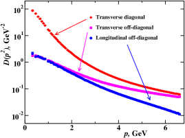
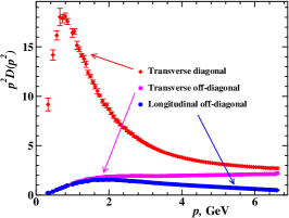
(a)	(b)

Figure 1: (a) The formfactors $D(p^{2})$, and (b) the gluon dressing functions, $p^{2}\,D(p^{2})$, vs. momentum, $p$.

One can see that all formfactors seem to tend to finite values as momentum goes to zero i.e. none of them is divergent or vanishing. The diagonal formfactor is dominating over the off–diagonal formfactors.

In Figure 1(b) the gluon dressing function, $p^{2}\,D(p^{2})$, is depicted. The diagonal (transverse) dressing function has a relatively narrow maximum at non–zero momentum $p^{\mathrm{diag}}_{0}\approx 0.7~{}\mathrm{GeV}$. Its behavior at small momenta is qualitatively very similar to the behavior of the gluon propagator in the Landau gauge (see e.g. [6]). The off-diagonal longitudinal dressing function has a wide maximum at $p^{\mathrm{offdiag}}_{0}\approx 2~{}\mathrm{GeV}$, while for the transverse off-diagonal dressing function formfactor it is a monotonically rising function for all available momenta.

One can compare the propagators obtained with the $U(1)$ gauge conditions (5) and (6). The first condition was implemented in Ref. [19] while the last one is adopted in the present paper. The comparison shows that the transverse diagonal propagators for these two gauge conditions coincide with each other at large momenta. At small momenta the formfactor obtained with Eq. (5) is slightly larger then the one calculated with Eq. (6). The difference at momentum $p=430~{}\mathrm{MeV}$ is about 15%. The formfactors for the off-diagonal gluons coincide with each other for all available momenta.

It is seen from Figure 1 that at $p\approx 6$ GeV dressing function $p^{2}\,D^{diag,offdiag}_{t,l}\approx 3$ and differ much from the free from $1/p^{2}$. The large renormalization of the formfactors in Landau gauge is discussed in Ref. [22]. There it has been shown that even three-loop corrections do not describe the behavior of the lattice gluon propagator at $p\approx 6$ GeV.

From Figures 1(a,b) it is clear that the off-diagonal gluon propagator is suppressed in comparison with the diagonal one. In Figure 2(a) we plot the ratio

$$R(p^{2})=\frac{D^{\mathrm{diag}}_{t}(p^{2})}{D^{\mathrm{offdiag}}_{t}(p^{2})}\,.$$ (13)

It is seen that the suppression of the off-diagonal propagator increases as the momentum decreases. This may be considered as an indication that in the MA gauge the diagonal gluons are responsible for physics in the infrared region.

From Figures 1(a,b) one may also notice that the formfactors $D^{\mathrm{offdiag}}_{t}(p^{2})$ and $D^{\mathrm{offdiag}}_{l}(p^{2})$ coincide at small momenta. In Figure 2(b) we plot the ratio

$$R_{\mathrm{offdiag}}(p^{2})=\frac{D^{\mathrm{offdiag}}_{t}(p^{2})-D^{\mathrm{offdiag}}_{l}(p^{2})}{D^{\mathrm{offdiag}}_{t}(p^{2})}\,.$$ (14)

One can see that $R_{\mathrm{offdiag}}$ decreases with decreasing momentum and vanishes at $p\sim 1$ GeV. This implies that in the IR region the off–diagonal propagator has the form

$$D^{\mathrm{offdiag}}_{\mu\nu}(p)\approx\delta_{\mu\nu}\cdot D_{t}^{\mathrm{offdiag}}(p^{2})\,,\quad p^{2}\lesssim 1~{}\mathrm{GeV}\,.$$ (15)

In order to characterize the propagators quantitatively we have fitted the formfactors in the infrared region by the following functions:

$$D(p^{2})= \frac{Z\,m^{2\alpha}}{{(p^{2}+m^{2})}^{1+\alpha}}\,,\qquad \mbox{(fit 1)}\,,$$ (16)

$$D(p^{2})= \frac{Z\,m^{2\alpha}}{p^{2(1+\alpha)}+m^{2(1+\alpha)}}\,,\qquad \mbox{(fit 2)}\,,$$ (17)

$$D(p^{2})= \frac{Z}{p^{2}+m^{2}}\,,\qquad \mbox{(Yukawa fit)}\,,$$ (18)

$$D(p^{2})= \frac{Z}{m^{2}+p^{2}+\kappa p^{4}/m^{2}}\,,\qquad \mbox{(Yukawa 2 fit)}\,,$$ (19)

$$D(p^{2})= \frac{Z\,p^{2}}{p^{4}+m^{4}}\,,\qquad \mbox{(Gribov fit)}\,.$$ (20)

where $Z$, $\alpha$ , $m$ and $\kappa$ are fitting parameters. The fitting functions (16),  (17),  (20) – after being modified to agree at large momenta with a known perturbation theory result – were used to fit the gluon propagator in Landau gauge [6]. It was concluded that function (17) provided the best fit. The fitting function (17) was also used in the compact U(1) theory and compact Abelian Higgs model [23] in three dimensions.

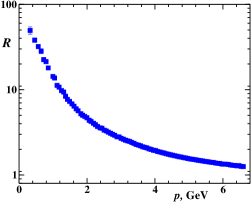
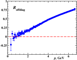
(a)	(b)

Figure 2: (a) The ratio of the transverse diagonal and off–diagonal components (13). (b) The ratio of the off–diagonal components (14) $vs.$ $p$.

The Yukawa fitting function, eq. (18), is introduced in order to compare our results with results of Refs. [14, 19], where such behavior was assumed for off-diagonal propagators. Another interesting possibility is to consider the momentum dependent mass in eq. (18), $m^{2}\to m^{2}(p^{2})$. Keeping only the lowest order of $p^{2}$ in $m^{2}(p^{2})$ expansion we get the fitting function (19) where $\kappa$ is an additional dimensionless parameter. Finally, we fit the data by the function (20) inspired by the Gribov proposal [24] for the Landau gauge.

The quality of the fitting result depends on the interval of momentum used in fitting. In this paper we restrict ourselves to the infrared region. We have chosen the interval starting from $p_{\min}=2\pi/(32a)=0.325~{}\mathrm{GeV}$ and ending at a variable value $p_{\max}$. For every fit we determine $p_{\max}$ as the highest momentum at which the data points corresponding to the lowest momenta are still consistent with the given fit. In other words, when momenta $p>p_{\max}$ are included in the fit the fitting curves go off the error bars of the lowest momenta data points. We employ this procedure for the diagonal propagator only, because the statistical weight of the infrared data points is low while the significance of these points is high. In the case of the off-diagonal propagators we have limited the region of fit by highest momentum $p_{\max}=1.7~{}\mathrm{GeV}$. The fits are shown in Figures 3(a-c) and the best fit parameters are presented in Table 1.

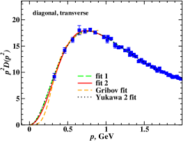
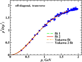
(a)	(b)
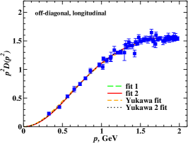
(c)

Figure 3: Fits of (a) transverse part of the diagonal propagator, (b) transverse and (c) longitudinal parts of the off-diagonal propagators, by the functions (16) and (17).

fit	$m$, GeV	$\alpha$ or $\kappa$	Z	$p_{\max},~{}\mathrm{GeV}$	$\chi^{2}/dof$
Transverse diagonal
fit 1	0.73(2)	0.92(3)	16.9(4)	1.7	0.8
fit 2	0.58(2)	0.49(5)	8.5(2)	1.0	0.4
Gribov fit	0.33(1)	-	4.58(5)	0.9	0.9
Yukawa 2 fit	0.50(2)	0.19(3)	8.3(3)	1.7	0.9
Transverse off-diagonal
fit 1	1.6(2)	0.6(2)	1.3(2)	1.7	1.0
fit 2	1.26(4)	0.19(4)	0.73(2)	1.7	1.0
Yukawa fit	1.08(2)	0	0.63(1)	1.7	1.5
Yukawa 2 fit	1.29(6)	0.15(5)	0.81(5)	1.7	1.0
Longitudinal off-diagonal
fit 1	1.4(2)	0.5(3)	1.0(3)	1.7	1.1
fit 2	1.14(6)	0.19(6)	0.63(3)	1.7	1.1
Yukawa fit	0.96(3)	0	0.52(1)	1.7	1.3
Yukawa 2 fit	1.14(8)	0.12(7)	0.66(6)	1.7	1.1

Table 1: The fitting results for the propagator formfactors at low momenta: best parameters of the fits (16–20). The corresponding highest momentum, $p_{\max}$, and $\chi^{2}/d.o.f.$ are also presented.

First we discuss the fits of the diagonal propagator. The three parameter fits (16,17,19) are working well and the corresponding curves are almost indistinguishable from each other, Figure 3(a). However, the fitting function (17) gives twice smaller value of $p_{\max}$ than the other functions, indicating that fit (17) works in a narrower region than the other fits. The mass parameters for these fits do not coincide, and the difference between them is about $30\%$.

We have also applied the two-parameter fits given by Yukawa (18) and Gribov (20) functions. The Gribov fit is working well for the diagonal propagator. One can see from Figure 3(a) that in order to discriminate the Gribov fitting function from the others we need the data at momenta smaller than available in our study. The Yukawa fit of the diagonal propagator does not work at all (we get $\chi^{2}/d.o.f.\sim 6$ for fits in $p_{\max}<1~{}\mathrm{GeV}$ region).

Concerning the transverse and longitudinal parts of the off-diagonal propagator one can make a few observations. First we notice, that the Gribov fitting function (20) is clearly not applicable for fitting of these propagators. Second, one can see that the formfactors for transverse and longitudinal parts almost coincide with each other at small momenta. The last fact implies that the best fit parameters for each particular type of the fits (16-19) must coincide as well,

$$m^{\mathrm{offdiag}}_{t}\approx m^{\mathrm{offdiag}}_{l}\,,\quad Z^{\mathrm{offdiag}}_{t}\approx Z^{\mathrm{offdiag}}_{l}\,,\quad\alpha^{\mathrm{offdiag}}_{t}\approx\alpha^{\mathrm{offdiag}}_{l}\,,\quad\kappa^{\mathrm{offdiag}}_{t}\approx\kappa^{\mathrm{offdiag}}_{l}\,,$$

in agreement with Table (1).

We have also found that the mass parameters in the off-diagonal gluon fits are approximately two times bigger then the corresponding parameters in the diagonal fit propagators:

$$m^{\mathrm{offdiag}}_{t,l}\approx 2m^{\mathrm{diag}}_{t}\,.$$

Thus, the off-diagonal propagator is clearly short–ranged compared to the diagonal one.

In Ref. [14] the off-diagonal propagator was successfully fitted in the infrared region of coordinate space by the Yukawa propagator. Our results (with respect to the off–diagonal propagator) indicate, that other fitting functions can also be used to describe this propagator.

Summarizing, we can say that the diagonal propagator can be fitted almost equally well with any of the three-parameter fits (16), (17) and (19). The same is true for the off-diagonal propagator. Among the two-parameter fits (20) is superior for the diagonal propagator while (18) is better for the off-diagonal one.

At smallest available momentum (325 MeV) the off-diagonal propagator is suppressed by the factor about 50 with respect to the diagonal one. Note that this suppression is only partially due to larger values of the mass parameter $m$ while equally or even more important role is played by smaller values of the parameter $Z$. We expect that the similar suppression exists also in the continuum theory because at our lattice spacing the renormalization effects for the $Z$–parameter are already quite small (according to Figure 1(a) the transverse diagonal and off–diagonal formfactors almost coincide with each other at largest available momentum).

5 Conclusions

Our results obtained in the Maximally Abelian gauge of $SU(2)$ gluodynamics clearly show that at low momenta the propagator of the diagonal gluon is much larger than the propagator of the off-diagonal gluons. This suggests that the colored objects at large distances interact mainly due to exchange by the diagonal gluons in agreement with the Abelian dominance property established in numerical studies of the MA gauge [16] for fundamental test charges.

The propagators do not show indications that they are either vanishing or divergent when $p\rightarrow 0$. To provide a quantitative description of the propagators at low momenta we fit the propagator formfactors using various functions. All infrared fits for both diagonal and off-diagonal propagators contain massive parameters, which are non-zero for both propagators. When the same fitting function is applied to the diagonal and off-diagonal formfactors the mass parameter for off-diagonal formfactor is more than twice bigger than that for the diagonal one. This is in a qualitative agreement with findings of Ref. [14]. But our more detailed analysis revealed that the difference in values of the mass parameters is not the only reason of the off-diagonal propagator suppression, the other reason is small values of parameter $Z$.

We have found that the diagonal propagator has qualitatively the same momentum dependence as the gluon propagator in Landau gauge while the off-diagonal propagator is very different. At small momenta the off-diagonal propagator is diagonal with respect to the space indices and thus defined by a single scalar function since its transverse and longitudinal formfactors become equal within error bars.

Appendix

The Maximally Abelian and the Abelian Landau gauges are defined as global maxima of the functionals (3) and (6), respectively. The global maxima is difficult to reach numerically and usually one finds several field configurations corresponding to local maxima of the gauge fixing functional and then the configuration with the highest value of the functional is chosen. The choice of the correct maximum, known as a Gribov problem [24], is crucial for the observables both in the MA gauge of $SU(2)$ gauge model [26] and in the Landau gauge of the U(1) gauge model [27].

Gauge fixing of the MA gauge with a careful treatment of the Gribov ambiguity was studied in Ref. [26]. In our investigation we follow this paper using the Simulated Annealing algorithm with 10 randomly generated gauge copies. The MA gauge fixing procedure is described in [26], and the Abelian Landau gauge fixing algorithm is briefly considered below.

To maximize the functional (6) we use the local over-relaxation algorithm with $\omega=1.8$, see, e.g., Ref. [28], with 20 randomly generated gauge copies. For the local gauge fixing we choose the following convergence criterion:

$${\cal G}(x)=|\sum_{\mu=1}^{4}\cos\varphi_{\mu}(x)\sin\theta_{\mu}(x)-\cos\varphi_{\mu}(x+\mu)\sin\theta_{\mu}(x+\mu)|\leq\varepsilon\,,$$ (A1)

where $\varepsilon$ is a small parameter. Note, that this condition must be satisfied at each site $x$ of the lattice.

To study the effects of the incomplete gauge fixing we chose the longitudinal part of the propagator of the diagonal gluon $D^{\mathrm{diag}}_{l}$ because it is most sensitive to the details of the gauge fixing procedure. According to the local gauge condition (4), $D^{\mathrm{diag}}_{l}$ must be zero when perfect numerical procedure is used. Its dependence on the convergence parameter $\varepsilon$ is presented in Figure 4(a). The propagator significantly depends on $\varepsilon$, especially in the region of small momenta. In our simulations we choose $\varepsilon=10^{-6}$.

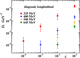
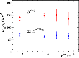
Figure 4: (a) The longitudinal part of the propagator of the diagonal gluon at various momenta $vs.$ convergence parameter $\varepsilon$; (b) the volume dependence of the diagonal and off-diagonal propagators at $p=0$, the corresponding lattice volumes are: $16^{4}$, $24^{4}$, $28^{4}$ and $32^{4}$.

We have also checked the dependence of $D^{\mathrm{diag}}_{t}$ on the number of gauge copies, $(N_{gc})$, used both in the MA and in the Abelian Landau gauge fixings. This check has been done using set of 30 configurations on $L=24$ lattice. Within error bars we have observed no dependence on the number of the MA gauge Gribov copies and we have found only very mild dependence on the number of the Abelian Landau gauge copies.

To check the finite volume effects we have calculated the propagators on different lattices at the same $\beta=2.40$. The transverse formfactors at zero momentum $D^{diag,offdiag}_{t}(0)$ were calculated as follows:

$$D^{diag,offdiag}_{t}(0)=\frac{1}{3}D^{diag,offdiag}_{\mu\mu}(0).$$ (A2)

We find that within error bars the values of the zero-momentum propagator are independent of the lattice volume, as can be seen from Figure 4(b).

We have also studied the volume dependence of the transverse part of the diagonal propagator at non–zero momenta. Since the finite volume affects mainly the low momentum region we have concentrated on the propagator at $p<1.5$ GeV. In Figure 5 we plot the transverse part of the diagonal propagator calculated on $24^{4}$ and $32^{4}$ lattices. It is seen that the volume dependence is very weak, it is within the error bars. The position of the maximum of $p^{2}D(p^{2})$ is the same for both lattices. The fit of the data for the propagator on $24^{4}$ lattice gives parameters which differs less than by $4\%$ from that given in Table 1 for $32^{4}$ lattice. Thus we estimate the systematic error induced by the finite volume effects to be less than $4\%$.

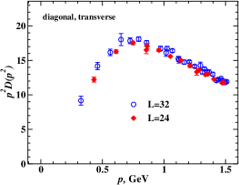
Figure 5: The transverse diagonal propagator at small momenta for the lattices $L=24$ and $L=32$.

References

- [1] S. Mandelstam, Phys. Rev. D 20 (1979) 3223; N. Brown and M. R. Pennington, Phys. Rev. D 39 (1989) 2723.
- [2] D. Zwanziger, Nucl. Phys. B 378 (1992) 525; Phys. Rev. D 65 (2002) 094039. L. von Smekal, R. Alkofer and A. Hauck, Phys. Rev. Lett. 79 (1997) 3591.
- [3] R. Alkofer and L. von Smekal, Phys. Rept. 353 (2001) 281.
- [4] P. Marenzoni, G. Martinelli and N. Stella, Nucl. Phys. B 455 (1995) 339.
- [5] A. Nakamura and S. Sakai, Prog. Theor. Phys. Suppl. 131 (1998) 585.
- [6] D. B. Leinweber et al., Phys. Rev. D 60 (1999) 094507.
- [7] F. D. Bonnet et. al, Phys. Rev. D 64 (2001) 034501.
- [8] H. Nakajima and S. Furui, arXiv:hep-lat/0208074.
- [9] C. Alexandrou, P. de Forcrand and E. Follana, Phys. Rev. D 65 (2002) 114508
- [10] J. M. Cornwall, Phys. Rev. D 26 (1982) 1453.
- [11] G. ’t Hooft, in High Energy Physics, ed. A. Zichichi, EPS International Conference, Palermo (1975); S. Mandelstam, Phys. Rept. 23, 245 (1976).
- [12] L. Del Debbio, M. Faber, J. Greensite and S. Olejnik, Phys. Rev. D 55 (1997) 2298.
- [13] M. N. Chernodub and M. I. Polikarpov, in ”Confinement, Duality and Non-perturbative Aspects of QCD”, p.387, Plenum Press, 1998, hep-th/9710205; R. W. Haymaker, Phys. Rept. 315 (1999) 153.
- [14] K. Amemiya and H. Suganuma, Phys. Rev. D 60 (1999) 114509.
- [15] Z. F. Ezawa and A. Iwazaki, Phys. Rev. D 25 (1982) 2681.
- [16] T. Suzuki and I. Yotsuyanagi, Phys. Rev. D 42 (1990) 4257.
- [17] M. Schaden, ”Mass generation in continuum SU(2) gauge theory in covariant Abelian gauges”, hep-th/9909011.
- [18] K. I. Kondo, Phys. Rev. D 58, 105019 (1998); Phys. Lett. B 514 (2001) 335; K. I. Kondo and T. Shinohara, Phys. Lett. B 491 (2000) 263; U. Ellwanger and N. Wschebor, ”Massive Yang-Mills theory in Abelian gauges, hep-th/0205057. D. Dudal and H. Verschelde, ”On ghost condensation, mass generation and Abelian dominance in the maximal Abelian gauge”, hep-th/0209025.
- [19] V. G. Bornyakov, S. M. Morozov and M. I. Polikarpov, “Gluon propagators in maximal abelian gauge of lattice gauge theory”, talk given at Lattice 2002, hep-lat/0209031.
- [20] G. ’t Hooft, Nucl. Phys. B 190 (1981) 455.
- [21] J. Fingberg, U. M. Heller and F. Karsch, Nucl. Phys. B 392 (1993) 493; Y. Koma et al., ”A fresh look on the flux tube in Abelian-projected gluodynamics”, hep-lat/0210014.
- [22] D. Becirevic, P. Boucaud, J. P. Leroy, J. Micheli, O. Pene, J. Rodriguez-Quintero and C. Roiesnel, Phys. Rev. D 60 (1999) 094509, hep-ph/9903364.
- [23] M. N. Chernodub, E. M. Ilgenfritz and A. Schiller, Phys. Rev. Lett. 88 (2002) 231601; Phys. Lett. B 555 (2003) 206, hep-lat/0212005; hep-lat/0208013, Phys. Rev. D, in press.
- [24] V. N. Gribov, Nucl. Phys. B 139 (1978) 1.
- [25] M. N. Chernodub and T. Suzuki, ”String breaking and monopoles”, hep-lat/0211026; hep-lat/0207018.
- [26] G. S. Bali, V. Bornyakov, M. Muller-Preussker and K. Schilling, Phys. Rev. D 54 (1996) 2863.
- [27] A. Nakamura and M. Plewnia, Phys. Lett. B 255 (1991) 274.
- [28] A. Cucchieri and T. Mendes, Nucl. Phys. B 471 (1996) 263.