Dynamical generation of a gauge symmetry
in the Double-Exchange model

Abstract

It is shown that a bosonic formulation of the double-exchange model, one of the classical models for magnetism, generates dynamically a gauge-invariant phase in a finite region of the phase diagram. We use analytical methods, Monte Carlo simulations and Finite-Size Scaling analysis. We study the transition line between that region and the paramagnetic phase. The numerical results show that this transition line belongs to the Universality Class of the Antiferromagnetic RP² model. The fact that one can define a Universality Class for the Antiferromagnetic RP² model, different from the one of the O($N$) models, is puzzling and somehow contradicts naive expectations about Universality.

, , , , , , , , and .

1 Introduction

The problem of the dynamical restoration of a gauge symmetry (see e.g. [1, 2] and references therein) has received considerable attention in the recent 10 years, because of the problem of introducing a chiral gauge theory in the lattice. Although the Ginsparg-Wilson [3] method has somehow superseded this approach, the question remains an interesting one. Naively, the problem could seem a trivial one [2]: the non gauge-invariant terms in the action generate a high-temperature-like gauge-invariant expansion with a finite radius of convergence. The subtle question is whether the radius of convergence of this expansion will remain finite in the continuum limit or not. In this letter, we want to address a related, but different question, namely, the generation of a local invariance in the low-temperature (broken-symmetry) phase of a system without any explicitly gauge-invariant term in the action. We have found this intriguing phenomenon in a numerical study of a simplified version of the Double-Exchange Model [4, 5](DEM), one of the most general models for magnetism in condensed matter physics, still under active investigation [6]. The local invariance does not follow from a high-temperature-like expansion, but from the infinite degeneracy of the ground-state (see next section), which occurs at a unique value of the control parameter at zero temperature, then extending to a finite region of the phase diagram at finite temperature. This phenomenon reminds one of the so-called Quantum-Critical Point phenomenology [7].

We have studied the model using Monte Carlo simulations and Finite-Size Scaling techniques [8, 9, 10]. We have found that the critical exponents are fully compatible with the ones [11] of the antiferromagnetic (AFM) RP² model in three dimensions [11, 12, 13], which has an explicit local Z₂ invariance. This might not be surprising, given the strong similarities in the ground-state of both models (see next section). However, the fact that one can explicitly show that there is a Universality Class associated to the AFM-RP² model is puzzling. Indeed, the most ambitious formulation of the Universality Hypothesis states that the critical properties of a system are fully determined by the space dimensionality and its symmetry groups at high-temperature ($\mathcal{G}$) and low-temperature ($\mathcal{H}$). Moreover, systems with a locally isomorphic $\mathcal{G}/\mathcal{H}$ are expected to have the same critical behavior. In our case, $\mathcal{G}$=O(3), and from our numerical study $\mathcal{H}$ seems to be O(2) [14], although the O(2) residual symmetry could be also broken (to O(1)=Z₂). In the former case, the Universality Class should be the one of the O(3) non-linear $\sigma$ model, while in the latter case one expects O(4) non-linear $\sigma$ model-like behavior [15]. Our results are definitely incompatible with an O(3)/O(2) scheme of symmetry breaking, and very hardly compatible with an O(4)/O(3) (locally isomorphic to O(3)/O(1)) scheme.

In recent years, the Universality Hypothesis (as stated above) has been challenged in a number of frustrated, chiral models [16]. Yet, detailed numerical simulations have shown that typical transitions are weakly first-order [17], which is hardly surprising, because the typical critical exponents proposed for chiral systems [16] are fairly similar to the effective exponents one expects in weak first-order transitions [18]. On the other hand, we have no doubt that the transition here studied is continuous, but we have no alternative explanation for our results.

2 The Model

Although some powerful techniques have been developed [19] for the Double-Exchange model [4] (involving dynamical fermions), lattice sizes beyond $L=16$ are extremely hard to study with the present generations of computers. Thus, one may turn to the simplified version proposed by Anderson [4], where a purely bosonic Hamiltonian is considered. This simplified model has been recently studied [5] by extensive Monte Carlo simulation. Yet, previous studies missed several phases in the phase diagram (see Fig. 1 and below).

Specifically, we consider a three dimensional cubic lattice of side $L$, with periodic boundary conditions. The dynamical variables, $\vec{\phi}_{i}$, live on the sites of the lattice and are three-component vectors of unit modulus. The Hamiltonian contains the Anderson version of the Double-Exchange model plus an antiferromagnetic first-neighbor Heisenberg interaction [20]:

$$-H=\sum_{<i,j>}J\vec{\phi}_{i}\cdot\vec{\phi}_{j}+\sqrt{1+\vec{\phi}_{i}\cdot\vec{\phi}_{j}}\,\quad,\quad J<0\,,$$ (1)

where $<\!i,j\!>$ means first-neighbor sites on the lattice. The partition function reads

$$Z=\int\mathrm{d}[\vec{\phi}]\,\e^{-H/T}\,,$$ (2)

the integration measure being the standard rotationally-invariant measure on the sphere. In the following, expectation values will be indicated as $\langle\dots\rangle$.

The zero temperature limit is dominated by the spin configurations that minimize the energy. Exploratory Monte Carlo simulations showed that these configurations have a bipartite structure. Indeed, let us call a lattice site even or odd, according to the parity of the sum of its coordinates ($\vec{r}_{i}=(x_{i},y_{i},z_{i})$, $x_{i}+y_{i}+z_{i}$ even or odd). Then the spins on the (say) even lattice are all parallel, while the spins on the odd sublattice are randomly placed on a cone of angle $\Omega$ ($\vec{\phi}_{i}\cdot\vec{\phi}_{j}=\cos\Omega$) around the direction of the even lattice. The energy when $T$ goes to zero is simply

$$H_{0}(\Omega)=-3L^{3}\left(J\cos\Omega+\sqrt{1+\cos\Omega}\right)\,.$$ (3)

Now, $\Omega(J)$ is obtained by minimizing $H_{0}(\Omega)$. For $J>-\sqrt{2}/4$, $\Omega=0$, meaning a ferromagnetic vacuum. For $-\sqrt{2}/4>J>-0.5$, one has $0<\Omega<\pi/2$ (ferrimagnetic vacuum), while for all $J<-0.5$, it is $\pi/2<\Omega<\pi$ (antiferrimagnetic vacuum). The full antiferromagnetic configuration ($\Omega=\pi$) is never stable at zero temperature. The $J=-0.5$ point is very peculiar: much like for the AFM-RP² model [13, 12, 11], spins in the even sublattice are randomly aligned or anti-aligned with the (say) $Z$ axis, while the spins in the odd sublattice are randomly placed in the $X,Y$ plane. Since spins in the two sublattices are perpendicular to each other, one can arbitrarily reverse every spin. A local Z₂ symmetry is dynamically generated and, as we will see, it extends to finite temperatures. An operational definition of dynamical generation of a gauge symmetry is the following. One must calculate the correlation-length for non gauge-invariant operators ($\xi_{\mathrm{NGI}}$) and compare it to the correlation-length corresponding to gauge-invariant quantities ($\xi_{\mathrm{GI}}$). In the continuum-limit ($\xi_{\mathrm{GI}}\to\infty$), one should have $\xi_{\mathrm{NGI}}/\xi_{\mathrm{GI}}\to 0$. We have checked that the correlation-length associated to the spin-spin correlation function (non Z₂ gauge-invariant) is smaller than $0.3$ for all temperatures at $J=-0.5$. The alert reader will notice that the symmetry group at the point $(T,J)=(0,-0.5)$ is rather a local O(2), besides the local Z₂ previously discussed. However, the associated correlation-length at finite temperature grows enormously when approaching the critical temperature (tenths of lattice-spacings already at $T=0.9T_{\mathrm{c}}$), and probably diverges. More details on this will be given in Ref. [14].

Figure 1: Phase diagram of the model (1), as obtained from Monte Carlo simulation. The labels correspond to paramagnetic (PM), ferromagnetic (FM), ferrimagnetic (FI), antiferrimagnetic (AFI), antiferromagnetic (AFM), and RP²-symmetric (RP²) phases.

A further analytical evidence for this fact can be obtained by performing a Taylor expansion of the action at $J=-1/2$ assuming that $\vec{\phi}_{i}\cdot\vec{\phi}_{j}$, which just vanishes at $J=-1/2$ and zero temperature, is small:

$$-H=1-{\textstyle\frac{1}{8}}\sum_{<i,j>}(\vec{\phi}_{i}\cdot\vec{\phi}_{j})^{2}+{\textstyle\frac{1}{16}}\sum_{<i,j>}(\vec{\phi}_{i}\cdot\vec{\phi}_{j})^{3}-{\textstyle\frac{5}{128}}\sum_{<i,j>}(\vec{\phi}_{i}\cdot\vec{\phi}_{j})^{4}+\ldots$$ (4)

We can assume that this expansion has a finite radius of convergence and so we can extend this series to the non zero temperature region. Notice that the first term in the expansion is just the AFM-RP² Hamiltonian modified by terms that are no longer gauge invariant (those with odd powers in the scalar product). We can argue that those terms, which break explicitly the gauge invariance, are irrelevant operators, in the Renormalization Group sense, at the PM to AFM-RP² critical point and so, our model at finite temperature should belong to the same Universality Class as the AFM-RP² model. Obviously, were the transition of the first order, the argument would not apply.

In the Z₂ gauge-invariant phase, the vectorial magnetizations defined as

$$\begin{array}[]{lcl}{\vec{M}}_{\mathrm{u}}&=&\frac{1}{L^{3}}\sum_{i}\vec{\phi}_{i}\,,\\ {\vec{M}}_{\mathrm{s}}&=&\frac{1}{L^{3}}\sum_{i}(-1)^{x_{i}+y_{i}+z_{i}}\vec{\phi}_{i}\,,\\ \end{array}$$ (5)

are zero. Thus, we define proper order parameters, invariant under that gauge symmetry, in terms of the spin field, $\vec{\phi}_{i}$ and the related spin-2 tensor field (which is $Z_{2}$ invariant):

$$\mathbf{\tau}_{i}^{\alpha\beta}=\phi_{i}^{\alpha}\phi_{i}^{\beta}-\frac{1}{3}\delta^{\alpha\beta}\quad,\quad\alpha,\beta=1,2,3\,.$$ (6)

Then we define:

$$\begin{array}[]{lcl}{\mbox{\boldmath$\tau$}}_{i}^{\mathrm{u}}&=&{\mbox{\boldmath$\tau$}}_{i}\,,\\ {\mbox{\boldmath$\tau$}}_{i}^{\mathrm{s}}&=&(-1)^{x_{i}+y_{i}+z_{i}}{\mbox{\boldmath$\tau$}}_{i}\,,\\ {\mathbf{M}}_{{\mathrm{u}},{\mathrm{s}}}&=&\frac{1}{V}\sum_{i}{\mbox{\boldmath$\tau$}}_{i}^{{\mathrm{u}},{\mathrm{s}}}\,.\end{array}$$ (7)

The different phases we find (see [14] for details) are: paramagnetic, ferromagnetic ($\langle{\vec{M}}_{\mathrm{u}}\rangle\neq 0$, $\langle{\vec{M}}_{\mathrm{s}}\rangle=0$), ferrimagnetic ($\|\langle{\vec{M}}_{\mathrm{u}}\rangle\|>\|\langle{\vec{M}}_{\mathrm{s}}\rangle\|>0$), antiferrimagnetic ($\|\langle{\vec{M}}_{\mathrm{s}}\rangle\|>\|\langle{\vec{M}}_{\mathrm{u}}\rangle\|>0$), antiferromagnetic ($\langle{\vec{M}}_{\mathrm{s}}\rangle\neq 0$, $\langle{\vec{M}}_{\mathrm{u}}\rangle=0$), and RP² ($\langle{\mathbf{M}}_{\mathrm{u}}\rangle,\langle{\mathbf{M}}_{\mathrm{s}}\rangle\neq 0$ but with vanishing vectorial magnetizations). The phase diagram can be seen in Fig. 1. Notice the strong similarities of the point $(T=0,J=-0.5)$ with a Quantum Critical Point [7]. A detailed analysis of this phase diagram will appear soon [14].

Let us end this section by defining the observables actually used in the simulation. They are obtained in terms of the Fourier transform of the tensor fields:

$$\widehat{\mathbf{T}}^{{\mathrm{u}},{\mathrm{s}}}_{p}=\sum_{\vec{r}\in L^{3}}\e^{-{\mathrm{i}}\vec{p}\cdot\vec{r}}\ {\mathbf{\tau}}^{{\mathrm{u}},{\mathrm{s}}}_{\vec{r}},$$ (8)

and their propagators

$$G_{{\mathrm{u}},{\mathrm{s}}}({\vec{p}})=\frac{1}{V}\left\langle{\mathrm{tr}}\widehat{\mathbf{T}}^{{\mathrm{u}},{\mathrm{s}}}_{\vec{p}}\widehat{\mathbf{T}}^{{\mathrm{u}},{\mathrm{s}}{\dagger}}_{\vec{p}}\right\rangle\,,$$ (9)

where

$$\vec{p}=\frac{2\pi}{L}\vec{n}\ ,\ n_{i}=0,\ldots,L-1\,.$$ (10)

Notice that $G_{\mathrm{u}}(0)=V{\mathrm{tr}}\langle({\mathbf{M}}_{\mathrm{u}})^{2}\rangle$, and $G_{\mathrm{u}}(\pi,\pi,\pi)=G_{\mathrm{s}}(0,0,0)=V{\mathrm{tr}}\langle({\mathbf{M}}_{\mathrm{s}})^{2}\rangle$. Then we have the usual ($\chi_{\mathrm{u}}$) and staggered ($\chi_{\mathrm{s}}$) susceptibilities,

$$\chi_{{\mathrm{u}},{\mathrm{s}}}=G_{{\mathrm{u}},{\mathrm{s}}}(0,0,0)\,.$$ (11)

Having those two order parameters, we must expect the following behavior for the propagators in the thermodynamic limit, in the scaling region and for $T>T_{\mathrm{c}}$:

$$\begin{array}[]{rcl}G^{{\mathrm{u}},{\mathrm{s}}}(\vec{p})&\simeq&\displaystyle\frac{Z_{{\mathrm{u}},{\mathrm{s}}}\xi_{{\mathrm{u}},{\mathrm{s}}}^{-\eta_{{\mathrm{u}},{\mathrm{s}}}}}{\vec{p}^{2}+\xi_{{\mathrm{u}},{\mathrm{s}}}^{-2}}\,,\\ \xi_{{\mathrm{u}},{\mathrm{s}}}&=&A_{{\mathrm{u}},{\mathrm{s}}}t^{-\nu}(1+B_{{\mathrm{u}},{\mathrm{s}}}t^{-\nu\omega}+\ldots),\end{array}$$ (12)

where $\xi_{\mathrm{u}}$ and $\xi_{\mathrm{s}}$ are correlation-lengths, $t=(T-T_{\mathrm{c}})/T_{\mathrm{c}}$ is the reduced temperature and $Z_{{\mathrm{u}},{\mathrm{s}}}$, $A_{{\mathrm{u}},{\mathrm{s}}}$ and $B_{{\mathrm{u}},{\mathrm{s}}}$ are constants. On the other hand, the anomalous dimensions $\eta_{\mathrm{u}}$ and $\eta_{\mathrm{s}}$ need not be equal: we can relate them to the dimensions of the composite operators following the standard way: $d-2+\eta_{\mathrm{u}}=2\mathrm{dim}({\mbox{\boldmath$\tau$}}^{\mathrm{u}})$ and $d-2+\eta_{{\mathrm{s}}}=2\mathrm{dim}({\mbox{\boldmath$\tau$}}^{{\mathrm{s}}})$, and in general $\mathrm{dim}({\mbox{\boldmath$\tau$}}^{{\mathrm{s}}})\neq\mathrm{dim}({\mbox{\boldmath$\tau$}}^{\mathrm{u}})$.

To study the propagators (12) on a finite lattice, we need to use the minimal momentum propagators

$$F_{{\mathrm{u}},{\mathrm{s}}}=\frac{1}{3}(G_{{\mathrm{u}},{\mathrm{s}}}(\pi/L,0,0)+\mathrm{(permutations)})\,.$$ (13)

With those quantities in hand, one can define a finite-lattice correlation-length [21] for the staggered, and non staggered sectors:

$$\xi_{{\mathrm{u}},{\mathrm{s}}}=\left(\frac{\chi_{{\mathrm{u}},{\mathrm{s}}}/F_{{\mathrm{u}},{\mathrm{s}}}-1}{4{\sin}^{2}(\pi/L)}\right)^{1/2}\,.\\$$ (14)

Other quantities of interest are the dimensionless cumulants

$$\kappa_{{\mathrm{u}},{\mathrm{s}}}=\frac{\langle\left({\mathrm{tr}}({\mathbf{M}}_{{\mathrm{u}},{\mathrm{s}}})^{2}\right)^{2}\rangle}{\langle{\mathrm{tr}}({\mathbf{M}}_{{\mathrm{u}},{\mathrm{s}}})^{2}\rangle^{2}}\,.$$ (15)

Besides the above quantities, we also measure the energy (1), which is used in a reweighting method [22], and temperature derivatives of operators through their crossed correlation with the energy.

3 Critical behavior

For an operator $O$ that diverges as $|t|^{-x_{O}}$, its mean value at temperature $T$ in a size $L$ lattice can be written, in the critical region, assuming the finite-size scaling ansatz as [8]

$$O(L,T)=L^{x_{O}/\nu}\left(F_{O}(\xi(L,T)/L)+O(L^{-\omega})\right),$$ (16)

where $F_{O}$ is a smooth scaling function and $\omega$ is the universal leading correction-to-scaling exponent.

In order to eliminate the unknown $F_{O}$ function, we use the method of quotients [9, 10, 11, 23]. One studies the behavior of the operator of interest in two lattice sizes, $L$ and $rL$ (typically $r=2$):

$$Q_{O}=O(rL,t)/O(L,t).$$ (17)

Then one chooses a value of the reduced temperature $t$, such that the correlation-length in units of the lattice size is the same in both lattices [11]. One readily obtains

$$\left.Q_{O}\right|_{Q_{\xi}=r}=r^{x_{O}/\nu}+O(L^{-\omega}).$$ (18)

Notice that the matching condition $Q_{\xi}=r$ can be easily tuned with a reweighting method. The usual procedure consists on fixing $r=2$, and obtaining the above quotients for several $L$ values in order to perform an infinite volume extrapolation.

In order to obtain the critical exponents, we use as operators $\chi_{{\mathrm{u}},{\mathrm{s}}}$ ($x_{\chi}=\gamma=2-\eta$), $\partial_{T}\xi_{\mathrm{s}}$ ($x_{\partial_{T}\xi_{\mathrm{s}}}=\nu+1$). Notice that several quantities can play the role of the correlation-length in Eq. (18): $\xi_{\mathrm{u}},\xi_{\mathrm{s}},L\kappa_{\mathrm{u}}$ and $L\kappa_{\mathrm{s}}$. This simply changes the amplitude of the scaling corrections, which will turn out to be quite useful.

Another interesting quantity is the shift of the apparent critical point (i.e. $r\xi(L,T_{\mathrm{c}}^{L,r})=\xi(rL,T_{\mathrm{c}}^{L,r})$), with respect to the real critical point:

$$T_{\mathrm{c}}^{L,r}-T_{\mathrm{c}}\propto\frac{1-r^{-\omega}}{r^{\frac{1}{\nu}}-1}L^{-\omega-\frac{1}{\nu}}\,.$$ (19)

4 The Simulation

We have studied the model (1) in lattices $L=6,8,12,16,24,32,48$ and $64$, with a Monte Carlo simulation at $J=-0.5$. The algorithm has been a standard Metropolis with 2 hits per spin. The trial new spin is chosen randomly in the sphere. The probability of finally changing the spin at least once is about $50\%$.

We have carried out 20 million full-lattice sweeps (measuring every 2 sweeps) at each lattice size at $T=0.056$. For the $L=64$ lattice we have also performed 20 million sweeps at $T=0.0558$. The largest autocorrelation time measured is about 1400 sweeps (corresponding to $\chi_{\mathrm{s}}$). To ensure the thermalization we have discarded a minimum of 150 times the autocorrelation time.

The computation was made on the RTN3 cluster of 28 1.9GHz PentiumIV processors at the University of Zaragoza and the total simulation time was equivalent to 11 months of a single processor.

5 Critical exponents

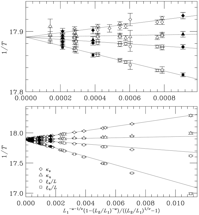
Figure 2: Shift of the apparent critical temperature Eq. (19) with the lattice size, using the four possible kinds of dimensionless operators: $\xi_{\mathrm{u}}/L$, $\xi_{\mathrm{s}}/L$, $\kappa_{\mathrm{u}}$ and $\kappa_{\mathrm{s}}$. The top panel is a magnification of the leftmost region. Only filled data points, corresponding to $r=2$, were used in the fit.

$L_{\mathrm{min}}$	$T_{\mathrm{c}}$	$\Delta T_{\mathrm{c}}$	$\omega$	$\Delta\omega$	$\chi^{2}/D$	$D$	$Q$
6	0.0559075	0.0000034	0.959	0.021	3.11	23	0.00
8	0.0558946	0.0000039	0.862	0.025	1.33	19	0.15
12	0.0558951	0.0000055	0.817	0.050	0.76	15	0.72
16	0.0558984	0.0000078	0.815	0.277	0.72	11	0.72

Table 1: Results of the infinite volume extrapolation with Eq. (19) to obtain $T_{\mathrm{c}}$ and $\omega$. $Q$ is the quality-of-fit parameter. Our final values are the bold values.

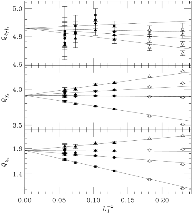
Figure 3: Quotients defined in Eq. (18), for $\partial_{T}\xi_{\mathrm{s}}$ (top), $\chi_{\mathrm{s}}$ (medium) and $\chi_{\mathrm{u}}$, as a function of $L^{-\omega}$, for $r=2$. We have measured at the crossing of four dimensionless operators, $\xi_{\mathrm{u}}/L$, $\xi_{\mathrm{s}}/L$, $\kappa_{\mathrm{u}}$ and $\kappa_{\mathrm{s}}$. Symbols are as in Fig. 2 .

$L_{\mathrm{min}}$	$\nu$	$\Delta\nu$	$\chi^{2}/D$	$D$	$Q$
6	0.7722	0.0041	2.55	23	0.00
8	0.7724	0.0055	1.66	19	0.03
12	0.7811	0.0107	1.03	15	0.42
16	0.7898	0.0179	0.83	11	0.61
	$\eta_{\mathrm{s}}$	$\Delta\eta_{\mathrm{s}}$
6	0.0238	0.0012	18.4	23	0.00
8	0.0278	0.0016	1.97	19	0.01
12	0.0315	0.0027	0.67	15	0.81
16	0.0359	0.0049	0.56	11	0.87
	$\eta_{\mathrm{u}}$	$\Delta\eta_{\mathrm{u}}$
6	1.3259	0.0013	8.52	23	0.00
8	1.3334	0.0018	1.56	19	0.06
12	1.3368	0.0031	0.77	15	0.72
16	1.3435	0.0058	0.62	11	0.82

Table 2: Infinite volume extrapolation for the critical exponents, using Eq. (18) and $\omega=0.82$. The fits were performed using $L\geq L_{\mathrm{min}}$. The goodness-of-fit ($Q$) is also indicated. The chosen extrapolation and error are emphasized.

The first step, as usual, is to estimate $\omega$ from Eq. (19). For this, one needs a rough-estimate of $\nu$. Since our data for the quotient of $\partial_{T}\xi_{\mathrm{s}}$ using $\xi_{\mathrm{s}}$ as correlation-length show very small scaling corrections (see Fig. 3), one can temporally choose $\nu=0.78$ and proceed with the determination of $\omega$. Having four possible dimensionless quantities, $\xi_{\mathrm{u}}/L$, $\xi_{\mathrm{s}}/L$, $\kappa_{\mathrm{u}}$ and $\kappa_{\mathrm{s}}$, we can perform a joint fit to Eq. (19) constrained to yield the same $T_{\mathrm{c}}$. This largely improves the accuracy of the final estimate. The full covariance matrix is used in the fit, and errors are determined by the increase of $\chi^{2}$ by one-unit. Our results are summarized in Fig. 2 and table 1. Although scaling corrections are clearly visible, good fits are obtained from $L_{\mathrm{min}}=12$. Thus, we conclude that

$$\omega=0.82(5)\ ,\ T_{\mathrm{c}}=0.055895(5)\,.$$ (20)

We are now ready for the infinite volume extrapolation of the critical exponents. As usual, one needs to worry about higher-order scaling corrections. Here we shall follow a conservative criterion: we shall perform the fit to Eq. (18) only for $L\geq L_{\mathrm{min}}$, and observe what happens varying $L_{\mathrm{min}}$. Once we found a $L_{\mathrm{min}}$ for which the fit is acceptable and the infinite volume extrapolation for $L\geq L_{\mathrm{min}}$ and $L>L_{\mathrm{min}}$ are compatible within errors, we take the extrapolated value from the $L\geq L_{\mathrm{min}}$ fit, and the error from the $L>L_{\mathrm{min}}$ fit. Our results can be found in Fig. 3 and in table 2. As well as for the critical temperature, we used all four dimensionless quantities in a single fit constrained to yield a common infinite volume extrapolation. Our final estimates are

$$\begin{array}[]{rclrclrcl}\nu&=&0.781(18)(1),&\eta_{\mathrm{s}}&=&0.032(5)(2),&\eta_{\mathrm{u}}&=&1.337(6)(7)\,,\end{array}$$ (21)

were the second error is due to the uncertainty in $\omega$.

One can compare these results with other models, once it is decided what is going to play the role of our $\eta_{\mathrm{u}}$ in the O($N$) models. Our candidate is the tensorial representation [9]

$$\begin{array}[]{lrclcclccl}\mathrm{RP}^{2}~{}\mbox{\cite[cite]{[\@@bibref{}{RP2D3}{}{}]}}:&\nu&=&0.783(11),&\eta_{\mathrm{s}}&=&0.038(3),&\eta_{\mathrm{u}}&=&1.339(10)\,,\\ \mathrm{O}(3)~{}\mbox{\cite[cite]{[\@@bibref{}{ON}{}{}]}}:&\nu&=&0.704(6),&\eta_{\phi}&=&0.0413(16),&\eta_{\vec{\phi}\otimes\vec{\phi}}&=&1.427(3)\,,\\ \mathrm{O}(4)~{}\mbox{\cite[cite]{[\@@bibref{}{ON}{}{}]}}:&\nu&=&0.748(9),&\eta_{\phi}&=&0.0384(25),&\eta_{\vec{\phi}\otimes\vec{\phi}}&=&1.374(5)\,.\end{array}$$ (22)

6 Conclusions

We have studied numerically a bosonic version of the DEM, Eq. (1), by Monte Carlo simulations, obtaining its full phase-diagram, missed in previous studies [5]. We have studied its critical behavior with Finite-Size Scaling techniques. As Eq. (21) and Eq. (22) show, our results for the critical exponents are fully compatible with the results for the AFM-RP² model, barely compatible with the O(4) model, and fully incompatible with the results for the O(3) model. Our results in the low temperature phase [14] seem to indicate that the scheme of symmetry-breaking is O(3)/O(2), which contradicts Universality. Most puzzling is the excellent agreement between the present results and the estimates for the AFM-RP² model. This seems to indicate that the AFM-RP² model really represents a new Universality Class in three dimensions, in plain contradiction with the Universality-Hypothesis (at least in its more general form). This seems to imply that the local isomorphism of ${\mathcal{G}}/{\mathcal{H}}$ is not enough to guarantee a common Universality Class. Of course, it could happen that we were seeing only effective exponents and that in the $L\to\infty$ limit a more standard picture arises. Yet, we do not find any obvious reason for two very different models to have such a similar effective exponents.

Another intriguing effect is that the augmented local $Z_{2}$ symmetry of the point $(T=0,J=-0.5)$ extends to the finite temperature plane, which is recalling a Quantum Critical Point [7]. Indeed, we find that the Universality Class is the one of an explicitly gauge-invariant model. To our knowledge this is a new effect in (classical) Statistical Mechanics, and deserves to be called dynamical generation of a gauge symmetry.

References

- [1] W. Bock, J. Smit and J.C. Vink, Nucl. Phys. B416 (1994) 645.
- [2] G. Parisi, Nucl. Phys. Proc. Suppl. 29BC (1992) 247.
- [3] P.H. Ginsparg, K.G. Wilson, Phys. Rev. B25 (1982) 2649; M. Lüscher, Lectures given at the International School of Subnuclear Physics, Erice (2000), hep-th/0102028.
- [4] C. Zener, Phys. Rev. 82 (1951) 403;P. W. Anderson and H. Hasegawa, Phys. Rev. 100 (1955) 675; P.-G. de Gennes, Phys. Rev. 118 (1960) 141.
- [5] Shan-Ho Tsai, D.P. Landau, J. of Mag. Mat. Mag. 226-230 (2001) 650 and J. of App. Phys. 87 (2000) 5807.
- [6] See e.g. E. Dagotto, T. Hotta and A. Moreo, Phys. Rep. 344 (2001) 1.
- [7] S. Sachdev, Quantum Phase Transitions, Cambridge University Press, Cambridge (1999); Science 288 (2000) 475.
- [8] J.L. Cardy Ed., Finite-Size Scaling. North-Holland, 1988.
- [9] H.G. Ballesteros, L.A. Fernández, V. Martín-Mayor, and A. Muñoz Sudupe, Phys. Lett. B387 (1996) 125.
- [10] H.G. Ballesteros, L.A. Fernández, V. Martín-Mayor, A. Muñoz Sudupe, G. Parisi and J.J. Ruiz-Lorenzo, J. Phys. A: Math. Gen. 32 (1999) 1.
- [11] H.G. Ballesteros, L.A. Fernández, V. Martín-Mayor, and A. Muñoz Sudupe, Phys. Lett. B378 (1996) 207; Nucl. Phys. B483 (1997) 707.
- [12] S. Romano, Int. J. of Mod. Phys. B8 (1994) 3389.
- [13] G. Korhing and R.E. Shrock, Nucl. Phys. B295 (1988) 36.
- [14] A. Cruz et al., in preparation.
- [15] P. Azaria, B. Delamotte and T. Jolicoeur, Phys. Rev. Lett. 64 (1990) 3175; P. Azaria, B. Delamotte, F. Delduc and T. Jolicoeur, Nucl. Phys. B408 (1993) 485.
- [16] See for example H. Kawamura, Can. J. Phys. 79 (2001) 1447, or A. Pelissetto, P. Rossi and E. Vicari Phys. Rev. B65 (2002) 020403, and references therein.
- [17] M. Itakura, cond-mat/0110306.
- [18] L.A. Fernández, M.P. Lombardo, J.J. Ruiz-Lorenzo and A. Tarancón, Phys. Lett. B277(1992) 485.
- [19] J.L. Alonso, L.A. Fernández, F. Guinea, V. Laliena and V. Martín-Mayor, Nucl. Phys. B569 (2001) 587.
- [20] J.L. Alonso, L.A. Fernández, F. Guinea, V. Laliena and V. Martín-Mayor, Phys. Rev. B63 (2001) 64416; J.L. Alonso, J.A. Capitán, L.A. Fernández, F. Guinea and V. Martín-Mayor, Phys. Rev.B 64 (2001) 54408.
- [21] F. Cooper, B. Freedman y D. Preston, Nucl. Phys. B 210 (1989) 210.
- [22] A.M. Ferrenberg and R.H. Swendsen, Phys. Rev. Lett. 61 (1988) 2635.
- [23] A. Pelissetto and E. Vicari, Phys. Rep. 368 (2002) 549.
- [24] J. Zinn-Justin, Quantum Field Theory and Critical Phenomena, Oxford University Press. First Edition 1989.