ITEP-LAT/2002–29
KANAZAWA 02–41
Finite temperature phase transition in lattice QCD with $N_{f}=2$ nonperturbatively improved Wilson fermions at $N_{t}=8$

Abstract

The finite temperature lattice QCD with $N_{f}=2$ nonperturbatively improved Wilson fermions is studied on $16^{3}8$ lattice. Using abelian projection after fixing to MA gauge we determine the transition temperature for $m_{\pi}/m_{\rho}\sim 0.8$.

1 Introduction

Determination of the critical temperature of the chiral phase transition is one of the important nonperturbative problems in QCD to be addressed in lattice simulations. Bielefeld group and CP-PACS collaborations using two different types of improved lattice action for fermions were able to estimate $T_{c}$ in the chiral limit and their values are in good agreement [1, 2]. Still there are many sources of systematic uncertainties and new computations of $T_{c}$ with different actions are useful as an additional check. We made first large scale simulations of the nonperturbatively $O(a)$ improved Wilson fermion action. Moreover we performed simulations with the lattice spacing $a$ substantially smaller than in studies by Bielefeld and CP-PACS groups.

The following fermionic action is employed in our study:

$$S_{F}=S^{(0)}_{F}-\frac{\rm i}{2}\kappa\,g\,c_{sw}a^{5}\sum_{x}\bar{\psi}(x)\sigma_{\mu\nu}F_{\mu\nu}\psi(x),$$ (1)

where $S^{(0)}_{F}$ is the original Wilson action, $c_{sw}$ is the clover coefficient determined nonperturbatively [3]. We use Wilson gauge field action.

The action (1) has been used in $T=0$ studies of lattice QCD by UKQCD and QCDSF collaborations [4, 5]. These studies confirmed that $O(a)$ lattice artifacts are suppressed as expected. To fix the physical scale and $m_{\pi}/m_{\rho}$ ratio we used results obtained by these collaborations [4]. So far only $N_{t}=4$ and $6$ finite temperature results obtained with action (1) are available [6]. These results were obtained at a rather large quark mass ($m_{\pi}/m_{\rho}>0.85$). In this work me make simulations with $N_{t}=8$ what allows us to decrease $m_{\pi}/m_{\rho}$ down to $\sim 0.8$. We choose the spatial extension of the lattice $N_{s}=16$ as a compromise between computational burden and need to reduce the finite size effects.

It is known that the order parameter of the finite temperature phase transition in quenched QCD is the Polyakov loop and the corresponding symmetry is global $Z(3)$ symmetry. In the chiral QCD the order parameter of the chiral symmetry breaking transition is the chiral condensate $<\bar{\psi}\psi>$. As numerical results show [1] both order parameters can be used to locate the transition point at intermediate values of the quark mass. We use Polyakov loop susceptibility to determine the transition temperature.

2 Simulation details

Hybrid Monte Carlo algorithm with parameters $\delta\tau=0.0125$, $n_{\tau}=20$, providing acceptance rates of about 70% is used in our simulations. The simulations were done on SR8000 Hitachi at KEK, Tsukuba and MVS 1000M at Joint Supercomputer Center, Moscow. For analysis SX5 NEC at RCNP and PC-cluster at ITP, Kanazawa were employed. Our code performs at the speed of 2.4 GFlops per node on Hitachi computer. We needed from 1000 ($\tau\equiv N_{traj}\cdot n_{\tau}\cdot\delta\tau=250$) to 3000 ($\tau=750$) trajectories for thermalization, depending on $\kappa$ and $\beta$. For runs started from configurations generated at the adjacent $\kappa$ this value was much lower. We determined the transition temperature at two values of $\beta$, 5.2 and 5.25, varying $\kappa$ as shown in Table 1.

$\beta=5.2,N_{s}=16$		$\beta=5.25,N_{s}=16$
$\kappa$	# of traj.	$\kappa$	# of traj.
0.1330	3409	0.1330	1540
0.1335	4500	0.1335	7439
0.1340	2100	0.13375	9225
0.1343	6650	0.1339	12470
0.1344	7485	0.1340	19479
0.1345	4647	0.1341	13750
0.1348	6013	0.13425	5155
0.1355	5650	0.1345	2650
0.1360	3699	0.1350	1780

Table.1  Simulation statistics.

We fixed the maximally abelian (MA) gauge on generated configurations. The simulated annealing algorithm has been used to fix the gauge. The advantages of this algorithm in comparison with the usual iterative algorithm has been demonstrated in $SU(2)$ pure gauge theory for MA gauge [8] and Maximal Center gauge [9].

Abelian and monopole Polyakov loops and their susceptibilities were measured on gauge fixed configurations. We found that for abelian and monopole observables the signal/noise ratio was better than that for gauge invariant nonabelian observables. This observation is in agreement with the results from quenched QCD at $T>0$ and both quenched and unquenched QCD at $T=0$. In particular the maximum of the Polyakov loop susceptibility is essentially better separated from the rest of the data for the monopole Polyakov loop than for nonabelian Polyakov loop. It is important that the transition temperature values determined by both susceptibilities are the same.

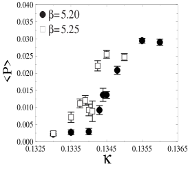
Figure 1: Nonabelian Polyakov loop at both $\beta$’s (left), and the abelian, monopole and photon Polyakov loops at $\beta=5.2$ (right).

3 Results and Conclusions

In Fig.1 we show results for average of various kinds of Polyakov loops. One can see that $\langle P\rangle$ is a smooth function of $\kappa$ and that abelian and monopole Polyakov loops behavior is qualitatively the same as behavior of the nonabelian Polyakov loop while the photon Polyakov loop is almost constant across the transition.

Transition point $\kappa$, denoted as $\kappa_{t}$, has been determined from the maximum of the Polyakov loop susceptibility, see Fig 2. As can be seen from Fig.2 the susceptibilities for abelian and monopole Polyakov loops have maxima at the same value of $\kappa$. We found that $\kappa_{t}=0.1344(1)$ at $\beta=5.2$ and $\kappa_{t}=0.1341(1)$ at $\beta=5.25$, see Fig.2. This was transformed into transition temperature with the help of the interpolation formula for $r_{0}/a$ [4]. The results are: $T_{c}r_{0}=0.54(2)$ and $0.56(2)$. In physical units, taking $1/r_{0}=394$ MeV, we obtained $T_{c}=213(10)$ and $222(10)$MeV, respectively. Using again data from [4] we estimate $m_{\pi}/m_{\rho}=0.78,0.82$ at the transition points.

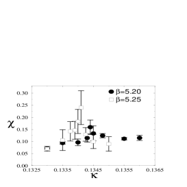
Figure 2: Nonabelian Polyakov loop susceptibilities at both $\beta$’s (left), abelian and monopole Polyakov loop susceptibilities at $\beta=5.2$ (right)

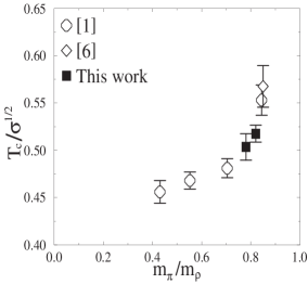
Figure 3: Transition temperature

In Fig.3 we show our results for transition temperature in comparison with results of refs. [1] and [6]. The ratio $T_{c}/\sqrt{\sigma}$ was computed for $\sqrt{\sigma}=425$ MeV used in [1]. We conclude that our results are in good qualitative agreement with previous results [1]. This agreement implies that the dependence of the transition temperature on the lattice spacing is rather weak.

For our lattice with $N_{s}/N_{t}=2$ the question of the finite volume effects is very important. To check this effect we made simulations at $\beta=5.2,\kappa=0.1343$ on $N_{s}=24$ lattice. The $\kappa$ value was chosen close to the transition point where finite volume effects should be more pronounced. We found that both average of the Polyakov loop and its susceptibility are the same within error bars as in our main simulations on $N_{s}=16$ lattice. This implies that the finite volume effects should not spoil our conclusions. We are planning to perform simulations on $24^{3}\cdot 10$ lattice at $m_{\pi}/m_{\rho}<0.7$ to determine $T_{c}$ closer to the chiral limit.

Acknowledgements
This work is partially supported by grants INTAS-00-00111, RFBR 02-02-17308, RFBR 01-02-117456, RFBR 00-15-96-786 and CRDF award RPI-2364-MO-02. We are very obliged to the staff of the Joint Supercomputer Center at Moscow and especially to A.V. Zabrodin for the help in computations. We thank Ph. De Forcrand, V. Mitrjushkin, M. Müller-Preussker for useful discussions. M.Ch. is supported by JSPS Fellowship grant No. P01023. V.B. acknowledges support by JSPS during period of work on this project.

References

- [1] F. Karsch, E. Laermann and A. Peikert, Nucl. Phys. B 605 (2001) 579 [arXiv:hep-lat/0012023].
- [2] A. Ali Khan et al. [CP-PACS Collaboration], action,” Phys. Rev. D 63 (2001) 034502 [arXiv:hep-lat/0008011].
- [3] K. Jansen and R. Sommer [ALPHA collaboration], Nucl. Phys. B 530 (1998) 185 [arXiv:hep-lat/9803017].
- [4] S. Booth et al. [QCDSF-UKQCD collaboration], Phys. Lett. B 519 (2001) 229 [arXiv:hep-lat/0103023].
- [5] C. R. Allton et al. [UKQCD Collaboration], Phys. Rev. D 65 (2002) 054502 [arXiv:hep-lat/0107021].
- [6] R. G. Edwards and U. M. Heller, Phys. Lett. B 462 (1999) 132 [arXiv:hep-lat/9905008].
- [7] O. Kaczmarek, F. Karsch, E. Laermann and M. Lutgemeier, Phys. Rev. D 62 (2000) 034021 [arXiv:hep-lat/9908010].
- [8] G. S. Bali, V. Bornyakov, M. Muller-Preussker and K. Schilling, Phys. Rev. D 54 (1996) 2863 [arXiv:hep-lat/9603012].
- [9] V. G. Bornyakov, D. A. Komarov and M. I. Polikarpov, Phys. Lett. B 497 (2001) 151 [arXiv:hep-lat/0009035].