Flavor Singlet Meson Mass in the Continuum Limit in Two-Flavor Lattice QCD

Abstract

We present results for the mass of the $\eta^{\prime}$ meson in the continuum limit for two-flavor lattice QCD, calculated on the CP-PACS computer, using a renormalization group improved gauge action, and Sheikoleslami and Wohlert’s fermion action with tadpole-improved $c_{\rm sw}$. Correlation functions are measured at three values of the coupling $\beta$ corresponding to the lattice spacing $a\approx 0.22,0.16,0.11$ fm and for four values of the quark mass parameter $\kappa$ corresponding to $m_{\pi}/m_{\rho}\approx 0.8,0.75,0.7,0.6$. For each $(\beta,\kappa)$ pair, 400-800 gauge configurations are used. The two-loop diagrams are evaluated using a noisy source method. We calculate $\eta^{\prime}$ propagators using both smeared and local sources, and find that excited state contaminations are much reduced by smearing. A full analysis for the smeared propagators gives $m_{\eta^{\prime}}=0.960(87)^{+0.036}_{-0.248}$ GeV in the continuum limit, where the second error represents the systematic uncertainty coming from varying the functional form for chiral and continuum extrapolations.

I Introduction

The large mass of the $\eta^{\prime}$ meson relative to members of the pseudoscalar octet has been an outstanding problem in low-energy hadron spectroscopy for some time weinberg ; metathooft ; wittenveneziano . A number of lattice QCD calculations has been carried out fukugitaetal ; itohetal ; kuramashietal ; duncanetal ; kilcup ; mcneile ; sesam to reproduce this feature, and to try to understand how it arises. These simulations, however, were made either with quenched configurations fukugitaetal ; itohetal ; kuramashietal ; duncanetal or, where full QCD was employed kilcup ; mcneile ; sesam , at a single lattice spacing. In this article we report on a two-flavor full QCD calculation of the flavor singlet meson mass including the continuum extrapolation. The calculation is made on a set of gauge configurations previously generated for a study of light hadron physics, the results of which have been reported in Ref. cppacsspectrum for meson and baryon spectra and in Ref. cppacsquarkmass for light quark masses. Three values of lattice spacing in the range $a\approx 0.22-0.11$ fm, and four values of quark mass covering $m_{\pi}/m_{\rho}\approx 0.8-0.6$ are used.

The main computational challenge in this work lies in the estimation of the the double quark loop diagram contribution to the $\eta^{\prime}$ propagator $G_{\eta^{\prime}}(t)$, for which the relative error $\Delta G_{{\eta^{\prime}}}(t)/G_{{\eta^{\prime}}}(t)$ increases quickly with $t$, the time separation from the source. If the error becomes large at a time slice $t_{\rm err}$ less than the first time slice of the plateau in the effective mass $t_{\mathrm{min}}$, it becomes undesirable to fit the $G_{{\eta^{\prime}}}$ directly. In such circumstances the ratio $G_{\eta^{\prime}}(t)/G_{\pi}(t)$ of $\eta^{\prime}$ to $\pi$ propagator has been used to try to cancel the effects of excited state contributions kilcup ; cppacspreliminary . In this work we set out to ensure a plateau, using an exponential-like smeared source and the method of $U(1)$ noise source noisenoise to decrease $t_{\mathrm{min}}$. The smearing technique has been previously employed in Refs. duncanetal ; kilcup ; mcneile ; sesam . We also calculate the disconnected contribution with a local source using the method of volume source without gauge fixing kuramashietal .

Preliminary results with the local source have been reported in Ref. cppacspreliminary . Here we present full results, and carry our analysis through in the case of the smeared source, where plateaux are achieved.

The organization of this article is as follows. Details of numerical calculations are described in Sec. II. In Sec. III, we give a full account of our analysis procedure and results including estimates of systematic errors arising from chiral and continuum extrapolations. Conclusions are given in Sec. IV.

II Numerical Calculations

II.1 Action and Configuration

Table 1: Overview of full QCD simulations. The lattice spacing $a$ is fixed by the vector meson mass at the physical quark mass and $M_{\rho}=768.4$ MeV. The set of trajectories used for flavor non-singlet hadrons cppacsspectrum ; cppacsquarkmass and measurements of $G_{\rm disc}$ with a local source cppacspreliminary is a subset of those referred to under $N_{\rm Traj}$.

$\beta$	$L^{3}\times T$	$a$ [fm]	$\kappa$	$m_{\rm PS}/m_{\rm V}$	$N_{\rm Traj}$	$N_{\rm Skip}$	$N_{\rm Smeared~{}Meas.}$
$c_{SW}$		$La$ [fm]
1.80	$12^{3}{\times}24$	0.2150(22)	0.1409	0.807(1)	6530	10	651
1.60		2.580(26)	0.1430	0.753(1)	5240	10	521
			0.1445	0.694(2)	7350	10	728
			0.1464	0.547(4)	5250	10	407
1.95	$16^{3}{\times}32$	0.1555(17)	0.1375	0.804(1)	7000	10	627
1.53		2.489(27)	0.1390	0.752(1)	7000	10	689
			0.1400	0.690(1)	7000	10	689
			0.1410	0.582(3)	5000	10	491
2.10	$24^{3}{\times}48$	0.1076(13)	0.1357	0.806(1)	4000	5	799
1.47		2.583(31)	0.1367	0.755(2)	4000	5	776
			0.1374	0.691(3)	4000	5	767
			0.1382	0.576(3)	4000	5	785

We use full QCD configurations for two flavors of dynamical quarks. In order to reduce discretization error, these configurations are generated with a renormalization-group (RG) improved gauge action and a mean field improved clover quark action. The RG-improved gauge action iwasakiaction has the form

$$S_{\rm RG}=\frac{\beta}{6}\left\{\;c_{0}\sum_{x,\mu<\nu}W_{\mu\nu}^{1\times 1}(x)+c_{1}\sum_{x,\mu,\nu}W_{\mu\nu}^{1\times 2}(x)\right\},$$ (1)

where $W^{i\times j}$ are Wilson loops with size $i\times j$, $c_{1}=-0.331$, and $c_{0}=1-8c_{1}$. For the clover quark action cloveraction , we set the coefficient $c_{\rm SW}=P^{-3/4}$, where $P$ is the plaquette value calculated in perturbation theory at one loop as $P=1-0.8412\beta^{-1}$.

A summary of the parameters and statistics is given in Table 1. We use three sets of configurations generated at bare gauge couplings $\beta=1.8$, 1.95, and 2.1, corresponding to the lattice spacings $a\approx 0.22$, 0.16 and 0.11 fm, with lattice dimensions $L^{3}\times T=12^{3}\times 24$, $16^{3}\times 32$ and $24^{3}\times 48$. The physical lattice sizes are roughly matched at $La\approx 2.5$ fm. At each $\beta$, four hopping parameters $\kappa$ are used. They correspond to $m_{\pi}/m_{\rho}\approx 0.8$, 0.75, 0.7 and 0.6. The lengths of runs range from 4000 to 7350 Hybrid Monte Carlo trajectories, and are listed under the column for $N_{\rm Traj}$ in Table 1.

II.2 Propagator Measurements

We calculate the single quark loop part of the $\eta^{\prime}$ meson propagator $G_{\rm conn}(t)$ ($=G_{\pi}(t)$) and the two quark loop part $G_{\rm disc}(t)$ both for local and smeared sources. The sink is always local. We use an exponential-like smearing kernel $K$

$$\begin{array}[]{rl}K(|\vec{n}-\vec{m}|\neq 0)&=Ae^{-B|\vec{n}-\vec{m}|}\\ K(0)&=1\end{array}$$

and parameters $A$ and $B$ are chosen to be the same as in Ref. cppacsspectrum . Gauge configurations are fixed to the Coulomb gauge.

We try applying source smearing to both, one or neither of the quark propagators. For the pion, Fig. 1 shows a case where smearing exactly one quark propagator delivers the earliest plateau. A comparison of ${\eta^{\prime}}$ propagators for different smearings can be found in Fig.2; again a preference for smearing is generally seen, although single smearing is not distinguished from double smearing as it was in the pion case. Since this trend holds over $(\beta,\kappa)$, we focus on the single-smeared-local combination for our analysis.

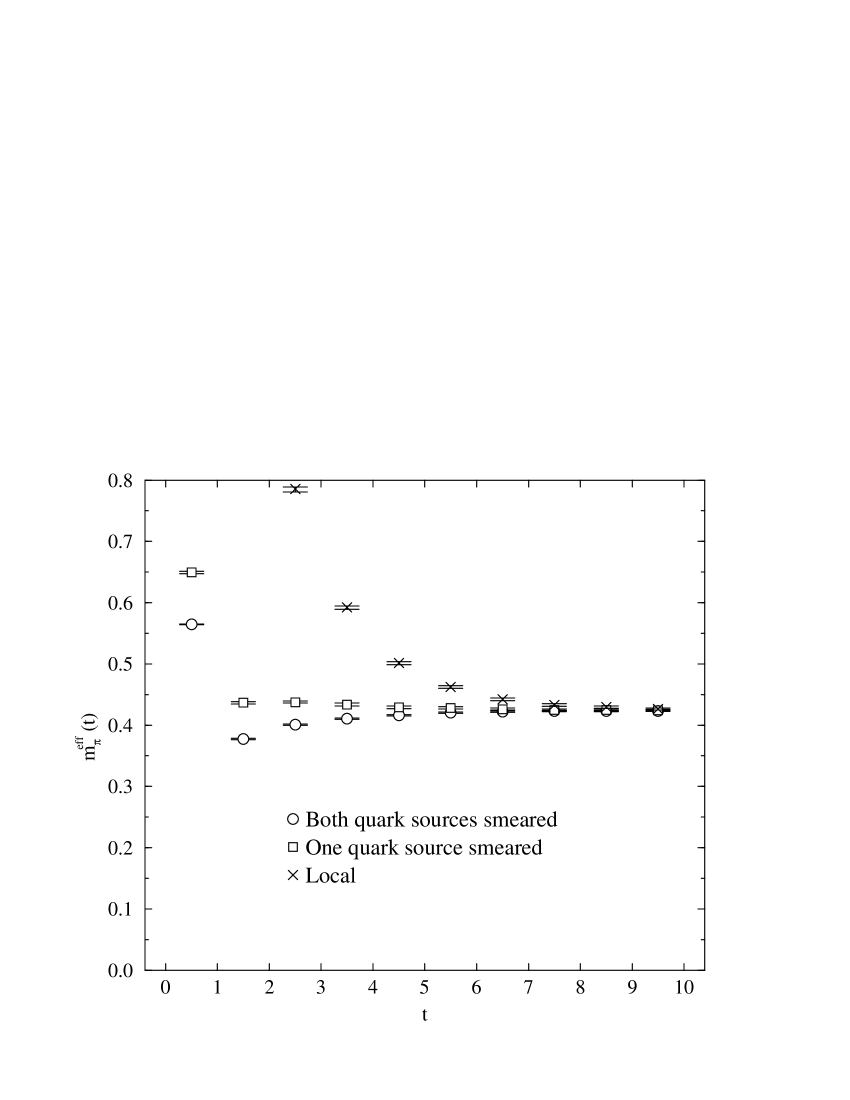
Figure 1: Comparison between smearing schemes for $\pi$ effective mass for $\beta=2.1$ and $\kappa=0.1374$ on a $24^{3}\times 48$ lattice.

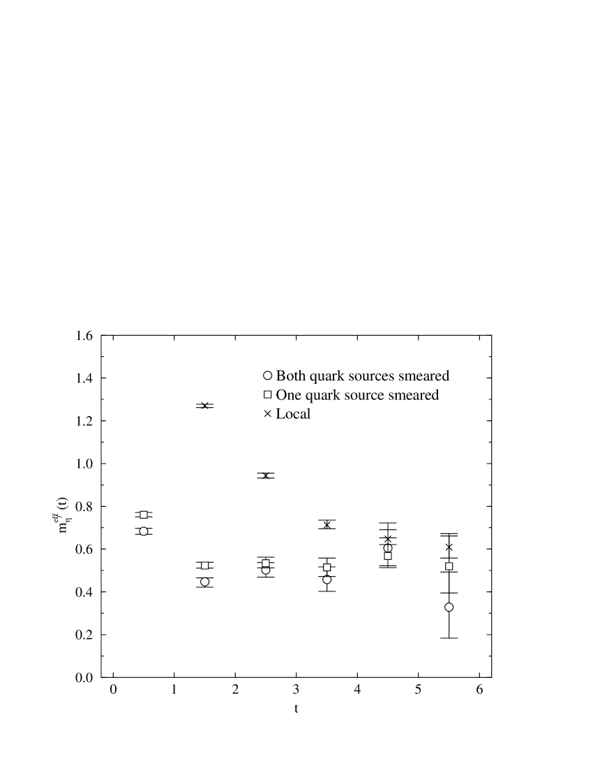
Figure 2: Comparison between smearing schemes for ${\eta^{\prime}}$ effective mass for $\beta=2.1$ and $\kappa=0.1374$ on a $24^{3}\times 48$ lattice.

Our implementation of the noisy source method is to use $U(1)$ random sources, fixing to the Coulomb gauge. A $U(1)$ random number $\exp(i\theta(\vec{n},t))$ is prepared for each site $(\vec{n},t)$ of the lattice, and a smeared source is made according to

$$\eta(\vec{n},t)=\sum_{\vec{m}}K(\vec{n}-\vec{m})\exp(i\theta(\vec{m},t)).$$ (2)

Combining the quark propagator $q(\vec{n},t)$ for the smeared source $\eta(\vec{n},t)$ with $\exp(-i\theta(\vec{n},t))$ yields the loop amplitude with a single smearing, while combining $q(\vec{n},t)$ with $\eta^{\dagger}(\vec{n},t)$ gives the doubly smeared amplitude.

Our noise sources are generated only at one value of the (spin, color) pair at a time; other spin and color components of the source are left at zero. The aim of this procedure is to decrease fluctuations. A similar procedure has been developed as the “spin explicit method” in smearonecomponent . In order to probe the gauge field evenly, we repeat 12 times, varying the spin-color index which is chosen to be non-zero over all its 12 possible values, generating a different noisy source for each. We repeat this whole process $N_{\rm noise}$ times, such that the total number of inversions for a fixed smearing is $N_{\rm inv}=N_{\rm noise}\times N_{\mathrm{spin}}\times N_{\mathrm{color}}$.

For the coarsest lattice at $\beta=1.8$ the noisy source measurement is made with four different values of $N_{\rm noise}$, 3, 5, 8 and 20. In Fig. 3 we show how the error in $G_{\rm disc}(t)$ varies as a function of $N_{\rm noise}$, taking $t=2$ as a representative time slice. In Fig. 4 a similar plot is shown for the $\eta^{\prime}$ meson mass obtained by fitting the $\eta^{\prime}$ propagator to a single hyperbolic cosine function. While the error is generally smaller for larger $N_{\rm noise}$ as expected, the precision increases only slowly with $N_{\rm noise}$, particularly for light quark masses. Furthermore these errors themselves fluctuate significantly. Overall, we cannot be certain that the $N_{\rm noise}$ reduction will benefit our result. Since $N_{\rm noise}$ and computer time are linearly related, we choose $N_{\rm noise}=3$ for measurements in the more costly cases of $\beta=1.95$ and 2.1. At $\beta=1.8$, we use $N_{\rm noise}=8$, since it gives the smallest observed error in the chiral limit.

Figure 3: Relative error of one-quark smeared $G_{\rm disc}(t=2)$ versus $N_{\rm noise}$ at $\beta=1.8$.

Figure 4: The same as Fig. 3 for relative error of $m_{\eta^{\prime}}$. Data at the chiral limit are also shown by crosses.

In our calculation with the local source cppacspreliminary , we evaluate $G_{\rm disc}$ with the volume source method without gauge fixing kuramashietal . This measurement is made for every trajectory. On the other hand, $G_{\rm conn}$ is measured every $N_{\rm Skip}$ trajectories, so an additional binning of $G_{\rm disc}$ is performed in preparation for constructing $G_{{\eta^{\prime}}}$.

We calculate errors of the propagator at each time separation by the jackknife method. In our study of flavor non-singlet hadrons cppacsspectrum , an autocorrelation analysis has shown that configurations separated by 50 trajectories are sufficiently decorrelated, so we use bins of 50 trajectories in the jackknife analyses, which translates into a bin size of 5 ($\beta=1.8$, 1.95) or 10 ($\beta=2.1$) measurements.

Slightly different numbers of configurations have been used for the ${\eta^{\prime}}$ in the smeared case. The number of measurements of smeared ${\eta^{\prime}}$ correlators for each $(\beta,\kappa)$ pair is given under the column for $N_{\rm Smeared~{}Meas.}$ in Table 1.

III Analysis and Result

III.1 Fitting of Propagators

To extract the $\eta^{\prime}$ meson mass, we fit the propagator using a single hyperbolic cosine function:

$$G_{\eta^{\prime}}(t)=A_{\eta^{\prime}}\left[\exp(-m_{\eta^{\prime}}t)+\exp(-m_{\eta^{\prime}}(T-t))\right],$$ (3)

where $T$ is the temporal lattice size. Alternatively one may fit the ratio $G_{\rm disc}(t)/G_{\pi}(t)$ to

$$\frac{G_{\rm disc}(t)}{G_{\pi}(t)}=1-B\exp(-\Delta m~{}t),$$ (4)

where $\Delta m=m_{\eta^{\prime}}-m_{\pi}$. The $\eta^{\prime}$ meson mass is then obtained by adding to $\Delta m$ the pion mass $m_{\pi}$ extracted from a standard fit of form

$$G_{\pi}(t)=A_{\pi}\left[\exp\left(-m_{\pi}t\right)+\exp\left(-m_{\pi}(T-t)\right)\right].$$ (5)

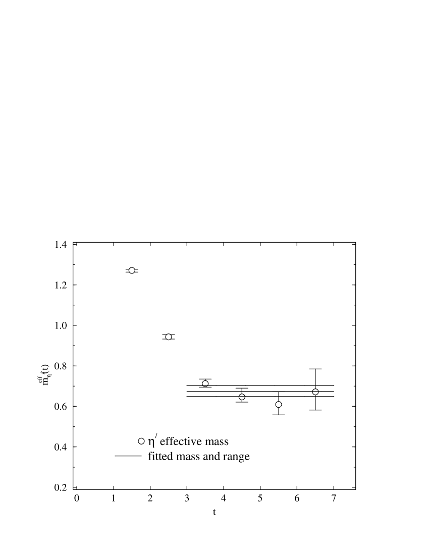
Figure 5: ${\eta^{\prime}}$ effective mass $m_{\eta^{\prime}}^{\rm eff}(t)$ obtained from local source at $\beta=2.1$ and $\kappa=0.1374$ on a $24^{3}\times 48$ lattice.

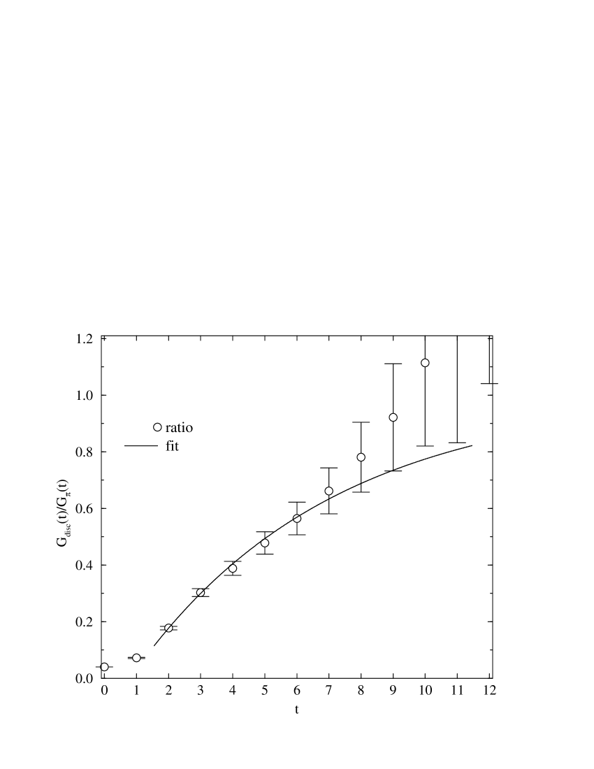
Figure 6: Ratio $G_{\rm disc}(t)/G_{\pi}(t)$ from local source for $\beta=2.1$ and $\kappa=0.1374$ on a $24^{3}\times 48$ lattice.

Let us first look at data obtained with the local source with the volume source method. Figure 5 shows the effective mass for the $\eta^{\prime}$ for a typical case of $(\beta,\kappa)=(2.1,0.1374)$ on a $24^{3}\times 48$ lattice. The $\eta^{\prime}$ effective mass does not show a clear plateau. We nonetheless try to fit the propagator for $3\leq t\leq 6$ for this example, in order to compare with the ratio method. Figure 6 shows the corresponding ratio as a function of time. A fit of form (4) over $t\geq t_{\rm min}$ yields stable values for $m_{\eta^{\prime}}$ when one varies $t_{\rm min}$ over $2\leq t_{\mathrm{min}}\leq 3$. This conceals an unquantifiable systematic error from the effect of excited states. In fact, we obtain $m_{\eta^{\prime}}=$ 0.670(26) from the direct fit, while 0.584(16) from the ratio fit, showing a 14% discrepancy.

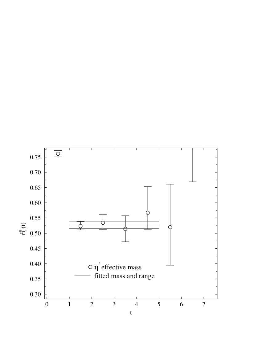
Figure 7: ${\eta^{\prime}}$ effective mass $m_{\eta^{\prime}}^{\rm eff}(t)$ from smeared source for $\beta=2.1$ and $\kappa=0.1374$ on a $24^{3}\times 48$ lattice.

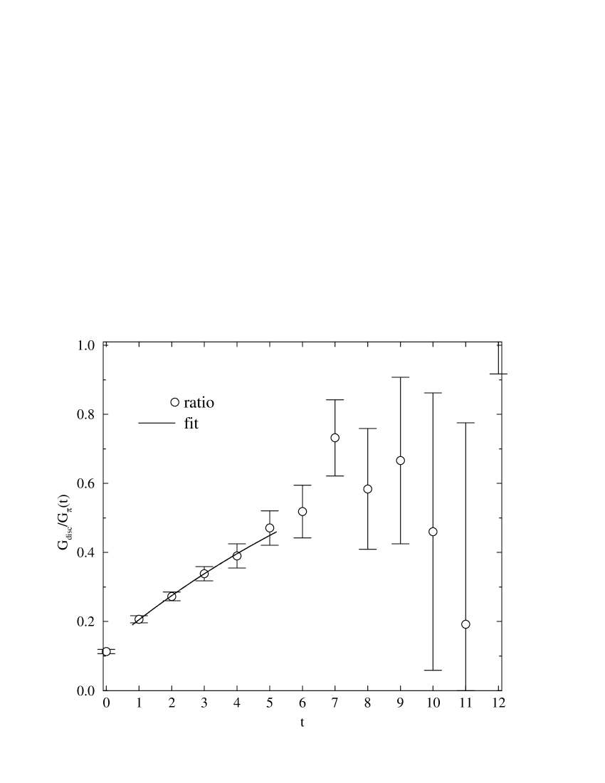
Figure 8: Ratio $G_{\rm disc}(t)/G_{\pi}(t)$ from smeared source for $\beta=2.1$ and $\kappa=0.1374$ on a $24^{3}\times 48$ lattice.

On the other hand, fitting propagators from the smeared source leads to more reliable estimate of $m_{\eta^{\prime}}$. We show in Fig. 7 the ${\eta^{\prime}}$ effective mass for smeared source for the same simulation parameter as that for local source above. There is an apparent plateau starting as early as $t_{\mathrm{min}}=1$. Fitting with $t_{\mathrm{min}}=1$ gives $m_{\eta^{\prime}}=$ 0.528(12). Figure 8 shows the corresponding ratio $G_{\rm disc}(t)/G_{\pi}(t)$ and the fit, which gives $m_{\eta^{\prime}}=$ 0.515(11). The difference of the two fits remains within 3%.

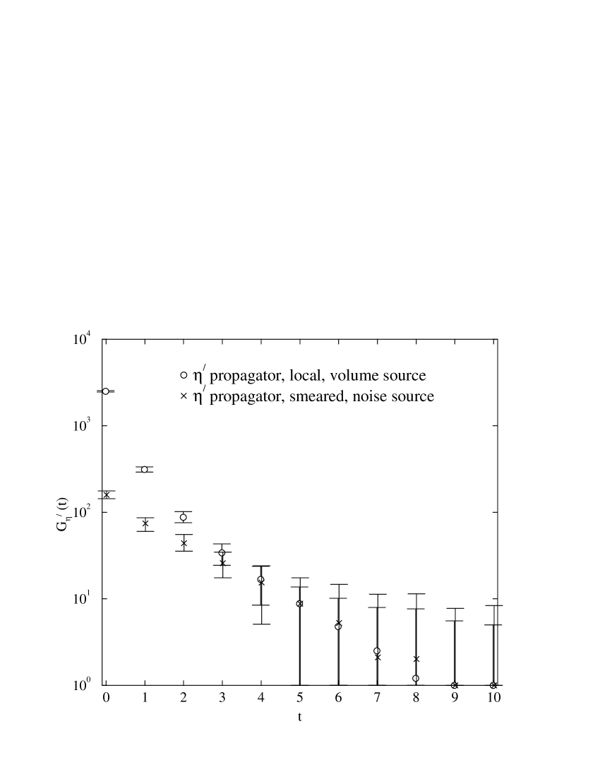
Figure 9: Comparison of ${\eta^{\prime}}$ propagator for local and smeared source for $\beta=2.1$ and $\kappa=0.1374$ on a $24^{3}\times 48$ lattice. The local source propagator has been normalized to be coincident with the smeared source propagator at t=5.

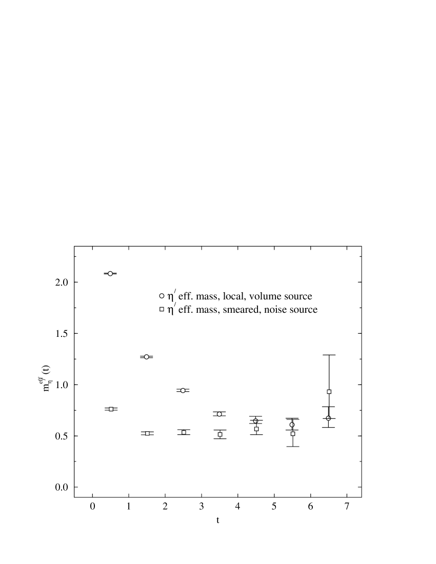
Figure 10: Comparison of ${\eta^{\prime}}$ effective mass for local and smeared source for $\beta=2.1$ and $\kappa=0.1374$ on a $24^{3}\times 48$ lattice.

In order to compare the quality of data from the local and smeared sources, we overlay two propagators and two effective masses in Figs. 9 and 10, respectively. The signal for $\eta^{\prime}$ in the smeared case has larger errors than the local case. On balance, however, the advantage of having plateaux in the smeared case, as shown in Fig. 10, greatly outweighs the disadvantage of its larger statistical error, which can at any rate be quantified. We therefore concentrate on data from smeared propagators in our full analyses.

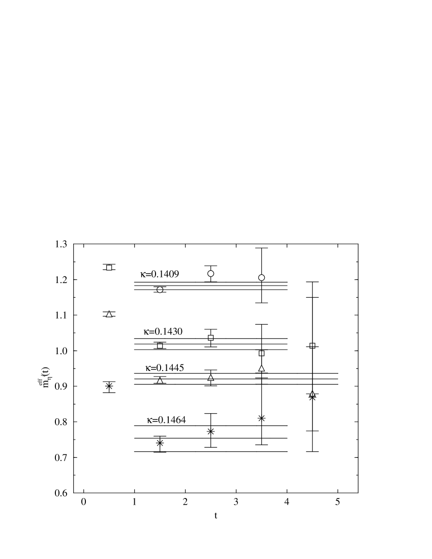
Figure 11: ${\eta^{\prime}}$ effective masses $m_{\eta^{\prime}}^{\rm eff}(t)$ from one-quark smeared sources for $\beta$=1.8 on a $12^{3}\times 24$ lattice.

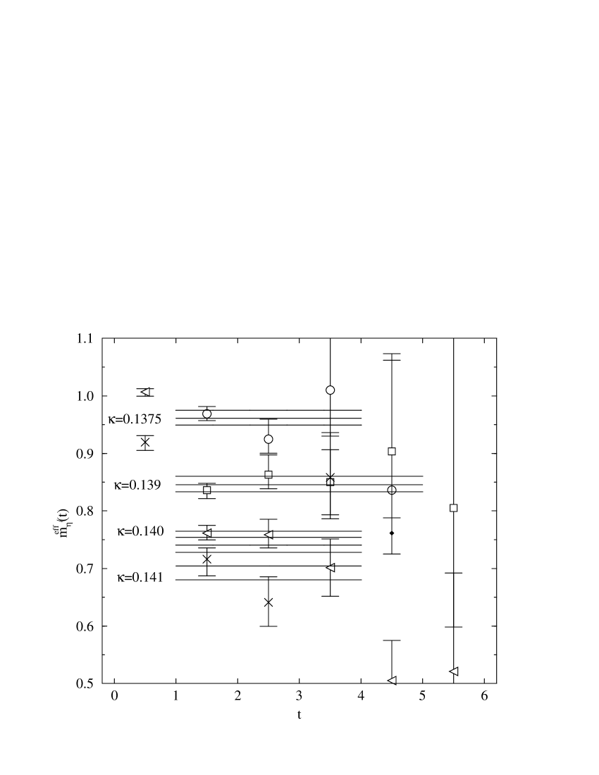
Figure 12: ${\eta^{\prime}}$ effective masses $m_{\eta^{\prime}}^{\rm eff}(t)$ from one-quark smeared sources for $\beta$=1.95 on a $16^{3}\times 32$ lattice.

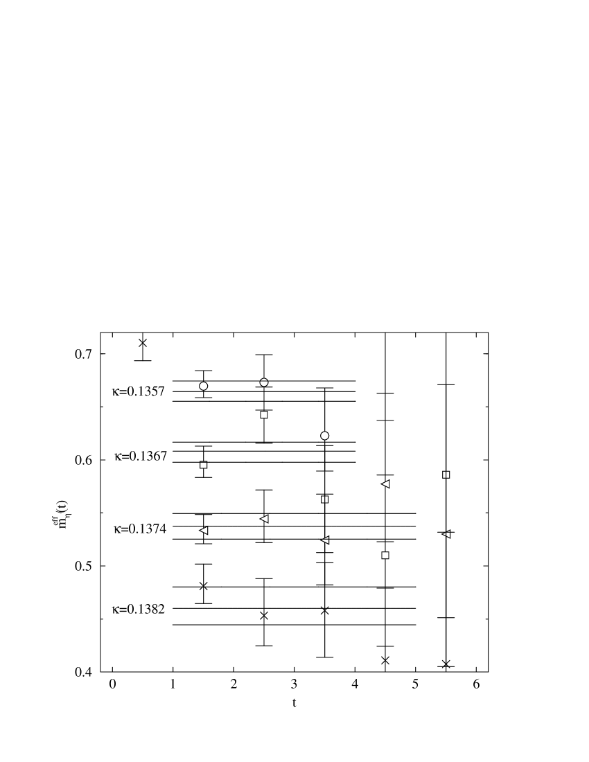
Figure 13: ${\eta^{\prime}}$ effective masses $m_{\eta^{\prime}}^{\rm eff}(t)$ from one-quark smeared sources for $\beta$=2.1 on a $24^{3}\times 48$ lattice.

Table 2: Fitted values of $m_{\pi}$ and $m_{\eta^{\prime}}$ for smeared source, with fit ranges.

$\beta$	$\kappa$	$am_{\pi}$	[$t_{\mathrm{min}},t_{\mathrm{max}}$]	$am_{\eta^{\prime}}$
				Direct Fit	[$t_{\mathrm{min}},t_{\mathrm{max}}$]	Ratio Fit	[$t_{\mathrm{min}},t_{\mathrm{max}}$]
$\beta=1.8$	$\kappa=0.1409$	1.155(1)	[5,12]	1.182(10)	[1,4]	1.218(8)	[1,4]
	$\kappa=0.1430$	0.984(1)	[6,12]	1.019(16)	[1,4]	1.057(11)	[1,5]
	$\kappa=0.1445$	0.821(1)	[6,12]	0.921(15)	[1,5]	0.937(15)	[1,5]
	$\kappa=0.1464$	0.532(2)	[6,12]	0.755(36)	[1,4]	0.769(35)	[1,5]
$\beta=1.95$	$\kappa=0.1375$	0.895(1)	[7,16]	0.960(13)	[1,4]	0.957(12)	[1,4]
	$\kappa=0.1390$	0.729(1)	[7,16]	0.846(13)	[1,5]	0.823(13)	[1,5]
	$\kappa=0.1400$	0.595(1)	[6,16]	0.754(12)	[1,4]	0.716(11)	[1,5]
	$\kappa=0.1410$	0.427(1)	[6,16]	0.705(24)	[1,4]	0.653(22)	[1,5]
$\beta=2.1$	$\kappa=0.1357$	0.630(1)	[10,24]	0.654(9)	[1,4]	0.680(10)	[1,4]
	$\kappa=0.1367$	0.516(1)	[10,24]	0.598(9)	[1,4]	0.602(9)	[1,5]
	$\kappa=0.1374$	0.424(1)	[10,24]	0.528(12)	[1,5]	0.515(11)	[1,5]
	$\kappa=0.1382$	0.295(1)	[10,24]	0.450(18)	[1,5]	0.426(18)	[1,5]

Effective masses from smeared propagator at every pair of $\left(\beta,\kappa\right)$ are plotted in Figs. 11 ($\beta=1.8$),  12 ($\beta=1.95$) and  13 ($\beta=2.1$). Consulting these effective masses, we determine $m_{\eta^{\prime}}$ from fitting to propagators with $t_{\rm min}=1$. Numerical values of $m_{\eta^{\prime}}$ are listed in Table 2.

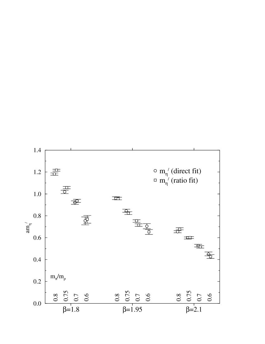
Figure 14: Comparison of ${\eta^{\prime}}$ effective mass from direct and ratio fit (smeared source).

For completeness, we carry out ratio fits to smeared propagators with $t_{\rm min}=1$. Numerical values are also given in Table 2. Comparison of results from the direct and ratio fits are made in Fig. 14. We find that the difference is contained within $8\%$. We should be aware that the $\pi$ effective mass does not exhibit a plateau as early as $t_{\rm min}=1$ even for the smeared source (see, e.g., Fig. 15). While the amount of decrease in the pion effective mass is small for the smeared source, the ratio fit involves systematic uncertainties of this origin. We therefore do not use ratio results in our final analyses.

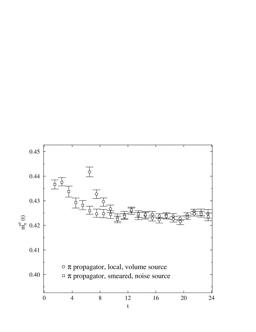
Figure 15: Comparison of pion effective mass for local and smeared source for $\beta=2.1$ and $\kappa=0.1374$ on a $24^{3}\times 48$ lattice.

III.2 Chiral Extrapolation

To chirally extrapolate the mass of the ${\eta^{\prime}}$, we test two functional forms. One is the form appropriate to a Nambu-Goldstone boson, with an extra constant term to reflect the non-zero mass of the ${\eta^{\prime}}$ in the chiral limit:

$$(am_{\eta^{\prime}})^{2}=A(am_{\pi})^{2}+B.$$ (6)

We refer to this form as NGB fit. Alternatively, one may take $\eta^{\prime}$ mass itself in a linear form in $(am_{\pi})^{2}$, which is standard for vector mesons (non-NGB. fit):

$$am_{\eta^{\prime}}=A(am_{\pi})^{2}+B.$$ (7)

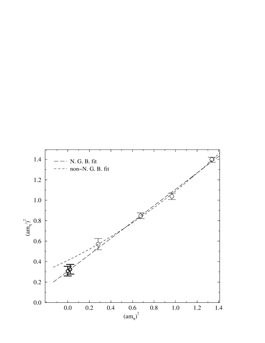
Figure 16: Chiral extrapolation for $\beta=1.8$ and smeared sources. The two extrapolated points correspond to physical and to zero pion mass.

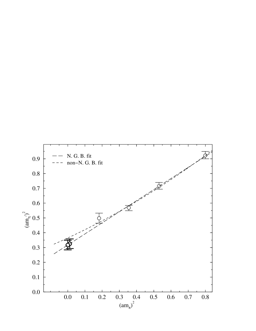
Figure 17: Chiral extrapolation for $\beta=1.95$ and smeared sources. The meaning of symbols is the same as in Fig. 16.

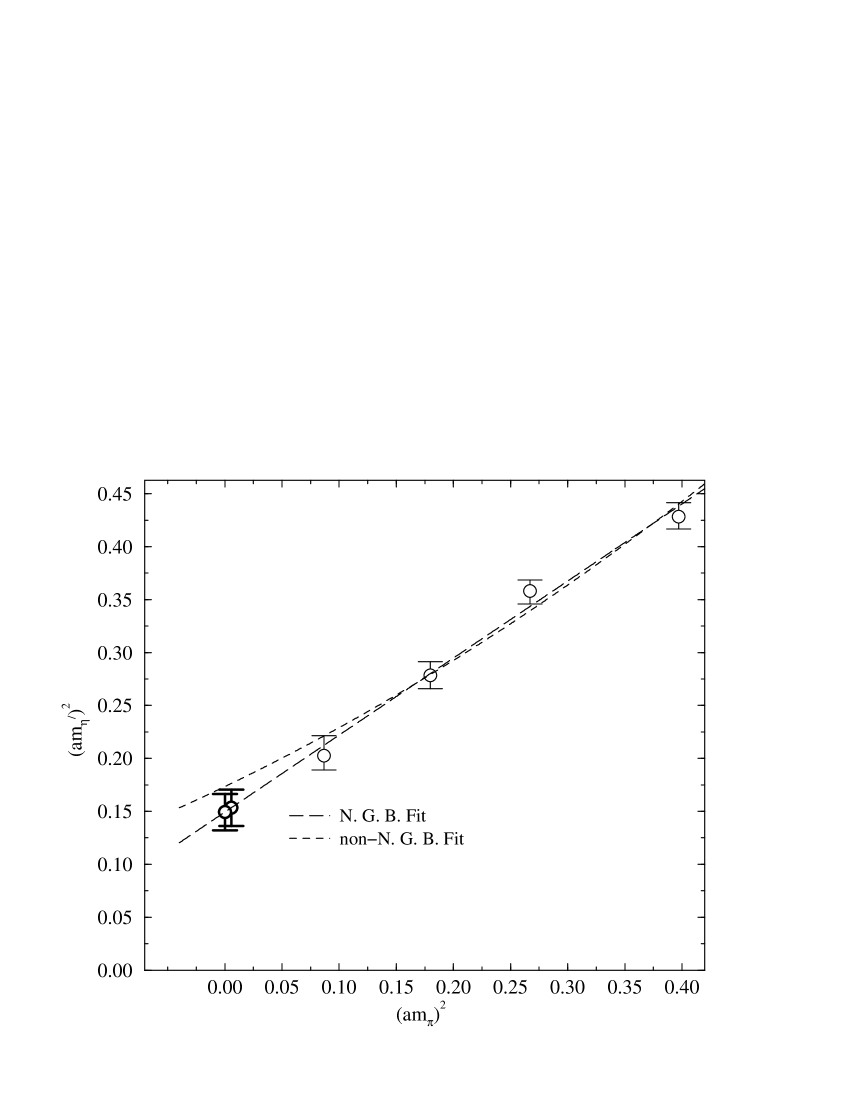
Figure 18: Chiral extrapolation for $\beta=2.1$, smeared sources. The meaning of symbols is the same as in Fig. 16.

Both fitting forms reproduce our data well with comparable $\chi^{2}/d.f.=$ 0.9–1.1 (NGB fit) and $\chi^{2}/d.f.=$ 0.4–2.2 (non-NGB fit), as shown in Figs. 16, 17 and 18. We use the NGB fit to determine the central values, while the non-NGB fit is used for estimation of systematic errors.

In order to extract $m_{\eta^{\prime}}$ at the physical point and in physical units, we follow the full spectrum analysis of Ref.cppacsspectrum and set the degenerate $u$ and $d$ quark masses and the lattice scale from the ratio of $\pi$ to $\rho$ mass $m_{\pi}/m_{\rho}=0.1757$ and the $\rho$ mass $m_{\rho}=0.7684~{}\,\mathrm{Ge\kern-1.00006ptV}$.

Table 3: Comparison of ${\eta^{\prime}}$ mass at the physical point from Eqs. (6) (NGB fit) and (7) (non-NGB fit).

$\beta$	$m_{\eta^{\prime}}({\rm GeV})$
	NGB	non-NGB
1.8	0.509(39)	0.589(24)
1.95	0.714(36)	0.766(26)
2.1	0.709(41)	0.764(30)

The ${\eta^{\prime}}$ meson mass at the physical point at each $\beta$ is given in Table 3. The Non-NGB fit leads to values of $m_{\eta^{\prime}}$ larger than the NGB fit. The difference is the largest for the coarsest lattice (16% which is about $2\sigma$) and smaller for the two finer lattices (8% or $1.5\sigma$ ). This difference yields a systematic error of about 4% ($0.4\sigma$) in the continuum limit, as discussed in detail in Sec. III.4.

III.3 Continuum Extrapolation

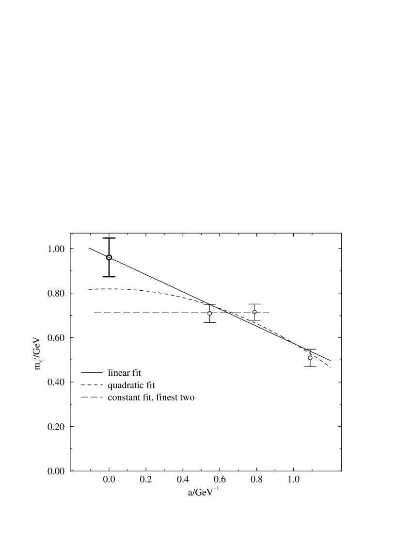
Figure 19: Continuum extrapolation of ${\eta^{\prime}}$ meson mass obtained with smeared sources.

Figure 19 shows $m_{\eta^{\prime}}$ as a function of $a$. We use a linear form for the continuum extrapolation,

$$m_{\eta^{\prime}}=C+Da$$ (8)

to estimate the central value in the continuum limit, since we employ a tadpole-improved value for the clover coefficient in our quark action. The $\chi^{2}/d.f.$ of the fit is 4.2. We also try a constant plus quadratic form, since one may expect ${\mathrm{O}}(a)$ effects which remain after tadpole improvement are small:

$$m_{\eta^{\prime}}=C+Da^{2}.$$ (9)

We find $\chi^{2}/d.f.$ of this fit to be 2.8. Finally, since the data hardly change between the finest two lattice spacings, we try removing the coarsest point and fitting to a constant. The quadratic and constant fits are used to estimate the systematic error.

Table 4: Systematic variations in $m_{\eta^{\prime}}$ over fit forms for chiral and continuum extrapolations.

	$m_{\eta^{\prime}}$(GeV)
central value	0.960(87)
quadratic continuum extrapolation	0.819(50)
constant continuum extrapolation	0.712(27)
non-N. G. B. chiral extrapolation	0.997(61)

III.4 Systematic Error Estimate and Final Result

We now consider the systematic errors based on the two variant forms for the continuum extrapolation, and the alternative form for the chiral extrapolation. In Table 4 we list the four estimates of masses in the continuum limit. The central value is obtained from the linear continuum extrapolation of results from the NGB fit. The quadratic continuum extrapolation gives a lower estimate, and the constant extrapolation a still lower one. On the other hand, the non-NGB chiral fit gives a raised estimate. We therefore take the difference between the central value and the value from the constant continuum extrapolation as the lower part of systematic error, and the deviation of the non-NGB chiral fit as the upper part.

Our final result for $m_{\eta^{\prime}}$ in the continuum limit reads

$$m_{\eta^{\prime}}=0.960(87)^{+0.036}_{-0.248}\mbox{\rm\ GeV}.$$ (10)

IV Conclusions

We have made the first calculation of the mass for the flavor singlet pseudoscalar meson in the continuum limit. We find that, using smearing, it becomes possible to fit the flavor singlet pseudoscalar meson correlator directly with a hyperbolic cosine ansatz. Similar conclusions have been reached in Refs. duncanetal ; sesam .

There is a lower systematic uncertainty of nearly $30\%$ in our final result. The systematic error breakdown indicates control over the continuum extrapolation to be the most important aim for future simulations, although this control may be established indirectly by some pattern of reduction in statistical error. On the other hand, the higher systematic error, coming entirely from the chiral extrapolation, is only $4\%$.

Our continuum result is in agreement with the experimental value for the ${\eta^{\prime}}$ mass of $m_{\eta^{\prime}}=0.956~{}{\rm GeV}$, despite the fact that our calculation is carried out for a flavor singlet meson composed of $u$ and $d$ quarks and within two-flavor approxaimation to QCD. Thus, calculations are underway to attempt to extract the elements of the mixing matrix between quark-based states and eigenstates of mass in the framework of the three-flavor QCD with a partially quenched strange quark. We also aim to follow this analysis with a continuum result from “2+1” flavor QCD, in which the strange quark is also treated dynamically, with similar or better statistics than the present work.

- (1) S. Weinberg, Phys. Rev. D11, 3583 (1975).
- (2) G. ’t Hooft, Phys. Rev. Lett. 37, 8 (1976).
- (3) E. Witten, Nucl. Phys. B156, 269 (1979); G. Veneziano, Nucl. Phys. B159, 213 (1979).
- (4) S. Itoh, Y. Iwasaki and T. Yoshié, Phys. Rev. D36, 527 (1987).
- (5) M. Fukugita, T, Kaneko and A. Ukawa, Phys. Lett. B154 (1984) 93.
- (6) Y. Kuramashi, M. Fukugita, H. Mino, M. Okawa and A. Ukawa, Phys. Rev. Lett. 72, 3448 (1994); M. Fukugita, Y. Kuramashi, M. Okawa and A. Ukawa, Phys. Rev. D51 (1995) 3952.
- (7) A. Duncan, E. Eichten, S. Perrucci, and H. Thacker, Nucl. Phys. B(Proc. Suppl.)53, 256 (1997); W. Bardeen, A. Duncan, E. Eichten, and H. Thacker, Phys. Rev. D62, 114505 (2000).
- (8) I. Venkataraman and G. Kilcup, Nucl. Phys. B(Proc. Suppl.)53, 259 (1997); hep-lat/971106 (1997).
- (9) C. Michael and C. McNeile, Phys. Lett. B491, 123 (2000).
- (10) T. Struckmann et al., Phys. Rev. D63, 074503 (2001).
- (11) CP-PACS Collaboration, A. Ali Khan et al., Phys. Rev. D65, 054505 (2002).
- (12) CP-PACS Collaboration, A. Ali Khan et al., Phys. Rev. Lett. 85, 4674 (2000).
- (13) CP-PACS Collaboration, A. Ali Khan et al., Nucl. Phys. B(Proc. Suppl.) 83, 162 (2000).
- (14) K. Bitar et al., Nucl. Phys. B313 348 (1989); H. R. Fiebig and R. M. Woloshyn, Phys. Rev. D42 3520 (1990).
- (15) Y. Iwasaki, Nucl. Phys. B258, 141(1985); University of Tsukuba preprint UTHEP-118 (1983) (unpublished).
- (16) B. Sheikoleslami and R. Wohlert, Nucl. Phys. B259, 572 (1985).
- (17) TXL Collaboration, S. Guesken et al., Phys. Rev. D59, 054504 (1999).