The Quark-Gluon Mixed Condensate $g\langle\bar{q}\sigma_{\mu\nu}G_{\mu\nu}q\rangle$ in SU(3)_c Quenched Lattice QCD

Abstract

Using the SU(3)_c lattice QCD with the Kogut-Susskind fermion at the quenched level, we study the quark-gluon mixed condensate $g\langle\bar{q}\sigma_{\mu\nu}G_{\mu\nu}q\rangle$, which is another chiral order parameter. For each current quark mass, $m_{q}=21,36$ and $52$ MeV, we generate 100 gauge configurations in the $16^{4}$ lattice with $\beta=6.0$, and perform the measurement of $g\langle\bar{q}\sigma_{\mu\nu}G_{\mu\nu}q\rangle$ at 16 points in each gauge configuration. Using the 1600 data for each $m_{q}$, we find $m_{0}^{2}\equiv g\langle\bar{q}\sigma_{\mu\nu}G_{\mu\nu}q\rangle/\langle\bar{q}q\rangle\simeq 2.5$ GeV² at the lattice scale in the chiral limit. The large value of $g\langle\bar{q}\sigma_{\mu\nu}G_{\mu\nu}q\rangle$ suggests its importance in the operator product expansion in QCD.

I Introduction

The main signature of the non-perturbative nature of quantum chromodynamics (QCD) is its nontrivial vacuum structure, which is represented by various condensates, or vacuum expectation values. For instance, the quark condensate $\langle\bar{q}q\rangle$ is a standard order parameter of spontaneous chiral symmetry breaking in QCD, and it determines properties of hadrons, especially the pion and the other pseudoscalar Nambu-Goldstone bosons. In the gluonic sector, the gluon condensate $\langle G_{\mu\nu}G^{\mu\nu}\rangle$ is an important quantity associated with the trace anomaly in QCD, and the topological susceptibility $\langle Q^{2}\rangle$ is responsible for the large $\eta^{\prime}$ mass due to the U_A(1) anomaly. Recently, the behavior of the various condensates at finite temperature/density is a subject of intensive research in the context of the QCD phase diagram, particularly the transition to the quark-gluon-plasma phase.

Among various condensates, we emphasize here the importance of the quark-gluon mixed condensate $g\langle\bar{q}\sigma_{\mu\nu}G_{\mu\nu}q\rangle\equiv{g\langle\bar{q}\sigma_{\mu\nu}G_{\mu\nu}^{A}\frac{1}{2}\lambda^{A}q\rangle}$. First, the mixed condensate represents a direct correlation between quarks and gluons in the QCD vacuum. In this point, the mixed condensate differs from the above-mentioned condensates even at the qualitative level. Second, this mixed condensate is another chiral order parameter of the second lowest dimension and it flips the chirality of the quark as

$$g\langle\bar{q}\sigma_{\mu\nu}G_{\mu\nu}q\rangle=g\langle\bar{q}_{R}\ (\sigma_{\mu\nu}G_{\mu\nu})\ q_{L}\rangle+g\langle\bar{q}_{L}\ (\sigma_{\mu\nu}G_{\mu\nu})\ q_{R}\rangle.$$ (1)

Note here that the mixed condensate plays a relevant role in the operator product expansion (OPE) in QCD as the next-to-leading chiral variant operator.

Also for the low-energy phenomena of hadrons, the mixed condensate is found to be important through the framework of the QCD sum rule SVZ , which connects the various condensates in OPE and the hadronic properties with the help of the dispersion relation. The condensates are determined phenomenologically so as to reproduce various hadronic properties systematically, considering the Borel stability of the sum rules RRY . For instance, in the standard QCD sum rule, the nucleon mass $m_{N}$ and the delta mass $m_{\Delta}$ are given in terms of $\langle\bar{q}q\rangle$ and $g\langle\bar{q}\sigma_{\mu\nu}G_{\mu\nu}q\rangle$ asIoffe ; Dosch

$$\lambda_{N}^{2}m_{N}e^{-m_{N}^{2}/M^{2}} = \frac{1}{(2\pi)^{2}}M^{4}(-\langle\bar{q}q\rangle)+0+{\cal O}(\mbox{7 dim. condensates}),$$ (2)

$$\lambda_{\Delta}^{2}m_{\Delta}e^{-m_{\Delta}^{2}/M^{2}} = \frac{4}{3(2\pi)^{2}}M^{4}(-\langle\bar{q}q\rangle)-\frac{2}{3(2\pi)^{2}}M^{2}(-g\langle\bar{q}\sigma_{\mu\nu}G_{\mu\nu}q\rangle)+{\cal O}(\mbox{7 dim. condensates})$$ (3)

$$= \frac{4}{3(2\pi)^{2}}M^{4}\left(1-\frac{m_{0}^{2}}{2M^{2}}\right)(-\langle\bar{q}q\rangle)+{\cal O}(\mbox{7 dim. condensates}),$$ (4)

where $M$ denotes the Borel mass and $\lambda_{N}$ and $\lambda_{\Delta}$ parameters in the QCD sum rule Ioffe ; Dosch . Here, we have used the standard parameterization as

$$m_{0}^{2}\equiv g\langle\bar{q}\sigma_{\mu\nu}G_{\mu\nu}q\rangle/\langle\bar{q}q\rangle.$$ (5)

In the QCD sum rules, the value $m_{0}^{2}\simeq 0.8\pm 0.2\ {\rm GeV}^{2}$ has been proposed as a result of the phenomenological analyses Bel ; RRY2 ; Ovchi ; Narison1 . Therefore, for the sum rule on $\Delta$, the second OPE term, which is proportional to the mixed condensate, amounts to the same magnitude to the leading OPE term, if we take the Borel mass $M$ equals to the typical baryon mass as $1$GeV. From these equations, one finds that the condensate $g\langle\bar{q}\sigma_{\mu\nu}G_{\mu\nu}q\rangle$ has large effects on the $N$-$\Delta$ splitting Dosch .

The condensate $g\langle\bar{q}\sigma_{\mu\nu}G_{\mu\nu}q\rangle$ is also important in the light-heavy meson systems Dosch2 , since the term $m_{H}\cdot g\langle\bar{q}\sigma_{\mu\nu}G_{\mu\nu}q\rangle$ proportional to the heavy quark mass $m_{H}$ contributes significantly in OPE of the corresponding sum rule. Furthermore, through the direct mixing of $q$, $\bar{q}$ and gluons, the mixed condensate $g\langle\bar{q}\sigma_{\mu\nu}G_{\mu\nu}q\rangle$ directly contributes in the exotic meson systems Latorre .

Needless to say, it is desirable to estimate $g\langle\bar{q}\sigma_{\mu\nu}G_{\mu\nu}q\rangle$, not only by the phenomenological parameter fitting in QCD sum rules, but also by a direct calculation from QCD. For this purpose, the lattice QCD Monte Carlo simulation Wilson is a powerful tool. With this method, the condensates can be directly calculated from QCD, keeping the non-perturbative effect. However, in spite of the importance of $g\langle\bar{q}\sigma_{\mu\nu}G_{\mu\nu}q\rangle$, there was only one preliminary lattice QCD study for $g\langle\bar{q}\sigma_{\mu\nu}G_{\mu\nu}q\rangle$ done about 15 years ago K&S . This pioneering study K&S gave an estimate $m_{0}^{2}\sim 1.1{\rm GeV}^{2}$, but this result is not conclusive yet because the simulation was done with insufficient statistics using a small and coarse lattice: the authors used only 5 gauge configurations on the $8^{4}$ lattice with $\beta=5.7$, and calculated the condensates at only 1 space-time point for each gauge configuration.

Therefore, in this paper, we present the calculation of $g\langle\bar{q}\sigma_{\mu\nu}G_{\mu\nu}q\rangle$ in lattice QCD with a large and fine lattice and with high statistics. We perform the measurement of $g\langle\bar{q}\sigma_{\mu\nu}G_{\mu\nu}q\rangle$ as well as $\langle\bar{q}q\rangle$ in the SU(3)_c lattice at the quenched level. Since these condensates are chiral order parameters, we adopt the Kogut-Susskind (KS) fermion, which keeps the explicit chiral symmetry in the massless quark limit. We generate 100 gauge configurations and pick up 16 space-time points for each configuration to calculate the condensates. Therefore, we obtain 1600 data for each quark mass and each $\beta$. We perform reliable estimate of the condensates with this high statistics.

This paper is organized as follows. In Sec. II, we explain our formalism to calculate the condensates. In Sec. III, we present the lattice QCD data, and discuss its reliability by performing several checks. Sec. IV is devoted to summary and concluding remarks.

II Formalism

In this section, we describe the formalism on the calculation of the condensates $\langle\bar{q}q\rangle$ and $g\langle\bar{q}\sigma_{\mu\nu}G_{\mu\nu}q\rangle$ in SU(3)_c quenched lattice QCD. Note that, even without the dynamical quark effects, the quenched lattice QCD calculations have reproduced various hadronic properties in good agreement with empirical values Rothe . Moreover, the characteristics of the quenched simulation are well under control owing to the accumulated knowledge. Therefore, it is worth performing the quenched lattice QCD calculation before proceeding to the full QCD calculation as a next step.

The lattice QCD is formulated in terms of the link-variable $U_{\mu}(s)\equiv\exp[-iagA_{\mu}(s)]$ on the lattice with spacing $a$, instead of the continuum gluon field $A_{\mu}(x)$. For the gauge sector, we adopt the standard Wilson action as

$$S_{G}=\sum_{s}\sum_{\mu>\nu}\beta\left[\ 1-\frac{1}{N_{c}}{\rm Re\ Tr\ }U_{\mu\nu}(s)\right],$$ (6)

with $\beta\equiv 2N_{c}/g^{2}$ and the plaquette operator $U_{\mu\nu}(s)$ on the $(\mu,\nu)$-plane, which is described by

$$U_{\mu\nu}(s)\equiv U_{\mu}(s)U_{\nu}(s+\mu)U^{\dagger}_{\mu}(s+\nu)U^{\dagger}_{\nu}(s).$$ (7)

For the fermion action, we adopt the KS-fermion. As the advantage of the KS-fermion, its action takes a simple form and preserves the explicit chiral symmetry in massless quark limit, $m=0$. The latter property of the KS-fermion is desirable for our study, since both of the condensates $\langle\bar{q}q\rangle$ and $g\langle\bar{q}\sigma_{\mu\nu}G_{\mu\nu}q\rangle$ are expected to be sensitive to explicit chiral symmetry breaking as chiral order parameters.

We comment here on the other lattice fermions briefly. The domain-wall fermion would be attractive from the viewpoint of chiral symmetry. However, its simulation is much more expensive in comparison with the KS-fermion. In addition, there are ambiguities originating from the newly introduced simulation parameters such as the domain-wall height. The Wilson and the clover fermions would not be appropriate for our purpose, because they have a serious disadvantage from the viewpoint of chiral symmetry. Specifically, the action for these fermions contains the term

$${\cal L}_{\rm E\chi SB}\propto\ \ \bar{q}(s)\left[\ U_{\mu}(s)q(s+\mu)+U^{\dagger}_{\mu}(s-\mu)q(s-\mu)-2q(s)\right],$$ (8)

which explicitly breaks chiral symmetry even for $m=0$. Although this term vanishes in the continuum limit, the chiral order parameters inevitably suffer the nontrivial contamination from this unphysical term at finite lattice spacing. This uncontrollable contamination should be avoided.

The action for the KS-fermion Rothe with the mass $m$ is described by

$$S_{F}=\frac{1}{2}\sum_{s,\mu}\eta_{\mu}(s)\bar{\chi}(s)\left[U_{\mu}(s)\chi(s+\mu)-U^{\dagger}_{\mu}(s-\mu)\chi(s-\mu)\right]+ma\sum_{s}\bar{\chi}(s)\chi(s),$$ (9)

where $\bar{\chi}$ and $\chi$ are Grassmann fields which have no spinor degrees of freedom, and $\eta_{\mu}(s)$ is the staggered phase defined as $\eta_{\mu}(s)\equiv(-1)^{s_{1}+\cdots+s_{\mu-1}}$, i.e.,

$$\eta_{1}(s)=1,\ \ \eta_{2}=(-1)^{s_{1}},\ \ \eta_{3}=(-1)^{s_{1}+s_{2}},\ \ \eta_{4}=(-1)^{s_{1}+s_{2}+s_{3}}.$$ (10)

In order to make the definition of the sign of $g\langle\bar{q}\sigma_{\mu\nu}G_{\mu\nu}q\rangle$ unambiguous, we note here that the definition of the continuum covariant derivative is $D_{\mu}\equiv\partial_{\mu}-igA_{\mu}$, corresponding to the definition of $U_{\mu}\equiv e^{-iagA_{\mu}}$.

In this formalism, the quark field $q$ is introduced as an ${\rm SU}(N_{f}=4)$ spinor field. The explicit relation between the quark field $q$ and the spinless Grassmann field $\chi$ is understood in the following way. When the gauge field is set to be zero, the quark field $q$ is expressed by

$$q_{i}^{f}(x) = \frac{1}{8}\sum_{\rho}\ (\Gamma_{\rho})_{if}\ \chi(x+\rho),$$ (11)

$$\Gamma_{\rho} \equiv \gamma_{1}^{\rho_{1}}\gamma_{2}^{\rho_{2}}\gamma_{3}^{\rho_{3}}\gamma_{4}^{\rho_{4}},$$ (12)

where $\rho=(\rho_{1},\rho_{2},\rho_{3},\rho_{4})$ with $\rho_{\mu}\in\{0,1\}$ runs over the 16 sites in the $2^{4}$ hypercube. The indices $i$ and $f$ denote the spinor and the flavor indices, respectively. When the gluon field is turned on, we insert additional link-variables in Eq. (11) in order to respect the gauge covariance.

The evaluation of the condensates amounts to the following expressions as

$$a^{3}\langle\bar{q}q\rangle = -\frac{1}{4}\sum_{f}{\rm Tr}\left[S^{f}(x,x)\right],$$ (13)

$$a^{5}g\langle\bar{q}\sigma_{\mu\nu}G_{\mu\nu}q\rangle = -\frac{1}{4}\sum_{f}\sum_{\mu,\nu}{\rm Tr}\left[S^{f}(x,x)\sigma_{\mu\nu}G_{\mu\nu}\right],$$ (14)

where the trace “${\rm Tr}$” is taken with respect to both the spinor and the color indices, and $S^{f}(y,x)$ denotes the Euclidean quark propagator for $f$-th flavor as

$$S^{f}(y,x)=\langle q^{f}(y)\bar{q}^{f}(x)\rangle.$$ (15)

In terms of $\chi$ and $\bar{\chi}$-fields, the flavor-averaged quark condensate is rewritten on the lattice as

$$a^{3}\langle\bar{q}q\rangle = -\frac{1}{2^{8}}\sum_{\rho}{\rm Tr}\left[\Gamma_{\rho}\Gamma_{\rho}^{\dagger}\ \langle\chi(x+\rho)\bar{\chi}(x+\rho)\rangle\right].$$ (16)

The corresponding diagram is shown in figure 1.

Figure 1: The diagrammatic representation of $\langle\bar{q}q\rangle$ in terms of the spinless Grassmann field $\chi$ on the lattice. The solid curve with the arrow denotes the propagation of $\chi$.

On the other hand, the flavor-averaged quark-gluon mixed condensate is given by

$$a^{5}g\langle\bar{q}\sigma_{\mu\nu}G_{\mu\nu}q\rangle = -\frac{1}{2^{8}}\sum_{\mu,\nu}\sum_{\rho}{\rm Tr}\left[\ {\cal U}_{\pm\mu,\pm\nu}(x+\rho)\ \Gamma_{\rho^{\prime}}\Gamma_{\rho}^{\dagger}\ \langle\chi(x+\rho^{\prime})\bar{\chi}(x+\rho)\rangle\ \sigma_{\mu\nu}\ G_{\mu\nu}^{\rm lat}(x+\rho)\ \right],$$

$$\rho^{\prime}\equiv\rho\pm\mu\pm\nu,$$

where the sign $\pm$ is taken such that the sink point $(x+\rho^{\prime})=(x+\rho\pm\mu\pm\nu)$ belongs to the same hypercube of the source point $(x+\rho)$. Here, in order to respect the gauge covariance, we have used in Eq. (II)

$${\cal U}_{\pm\mu,\pm\nu}(x)\equiv\frac{1}{2}\left[\ U_{\pm\mu}(x)U_{\pm\nu}(x\pm\mu)+U_{\pm\nu}(x)U_{\pm\mu}(x\pm\nu)\ \right],$$ (18)

where we use the definition of $U_{-\mu}(x)\equiv U^{\dagger}_{\mu}(x-\mu)$.

On the gluon field strength $G_{\mu\nu}$, we adopt the clover-type definition on the lattice,

$$G_{\mu\nu}^{\rm lat}(s)=\frac{i}{16}\sum_{A}\lambda^{A}\ {\rm Tr}\left[\lambda^{A}\{U_{\mu\nu}(s)+U_{\nu\,-\!\mu}(s)+U_{-\!\mu\,-\!\nu}(s)+U_{-\!\nu\,\mu}(s)\}-\lambda^{A}\{\mu\leftrightarrow\nu\}\right],$$ (19)

where $\lambda^{A}$ ($A=1,2,\cdots,8$) denotes the color SU(3) Gell-Mann matrix normalized as $\mbox{Tr}(\lambda^{A}\lambda^{B})=2\delta^{AB}$. In figure 2, we show the diagrams corresponding to Eqs. (II) and (19).

Figure 2: The diagrammatic representation of the two ingredients in $g\langle\bar{q}\sigma_{\mu\nu}G_{\mu\nu}q\rangle$ in terms of the spinless Grassmann field $\chi$ and the gluon field on the lattice. (a) The left diagram shows the propagation of $\chi$, with the insertion of gauge links. The solid curve with the arrow denotes the propagation of $\chi$, and the curly lines denote the inserted gauge link ${\cal U}_{\mu,\nu}$. (b) The right diagram shows the gluon field strength $G_{\mu\nu}^{\rm lat}$, where each loop of the curly line denotes a plaquette operator.

In the continuum limit, Eq. (19) leads to

$$G_{\mu\nu}^{\rm lat}(s)\rightarrow a^{2}\left[\ gG^{A}_{\mu\nu}(s)\frac{\lambda^{A}}{2}+{\cal O}(a^{2})\ \right].$$ (20)

It is worth mentioning that this definition has no ${\cal O}(a)$ discretization error. On the other hand, in Ref.K&S , the authors adopted a simple insertion of the gluon field strength,

$$a^{5}g\langle\bar{q}\sigma_{\mu\nu}G_{\mu\nu}q\rangle = \frac{1}{4}\sum_{f}\bar{q}^{f}(s)\sigma_{\mu\nu}U_{\mu}(s)U_{\nu}(s+\mu)q^{f}(s+\mu+\nu),$$ (21)

which contains ${\cal O}(a)$ error. Although both of the definitions, Eqs. (II) and (21), coincide to the $g\langle\bar{q}\sigma_{\mu\nu}G_{\mu\nu}q\rangle$ in the continuum limit, our definition of $G_{\mu\nu}$ will give less systematic errors in the actual lattice simulations with finite lattice spacing $a$.

III The lattice QCD results

III.1 Lattice QCD results for $g\langle\bar{q}\sigma_{\mu\nu}G_{\mu\nu}q\rangle$

We calculate the condensates $\langle\bar{q}q\rangle$ and $g\langle\bar{q}\sigma_{\mu\nu}G_{\mu\nu}q\rangle$ using the SU(3)_c lattice QCD at the quenched level. The Monte Carlo simulation is performed with the standard Wilson action for $\beta=5.7,5.8$ and $6.0$ on the $8^{4},12^{4}$ and $16^{4}$ lattice, respectively. The pseudo-heat-bath algorithm is adopted for the update of the gauge configuration. After 1000 sweeps for the thermalization, we pick up 100 gauge configurations for every 500 sweeps. The lattice unit $a$ is determined so as to reproduce the string tension $\sigma=0.89{\rm GeV/fm}$ rabbit:3Q . In Table 1, we summarize the lattice parameters for the gauge configuration. We note that the physical volume $V$ is roughly the same for the three calculations with different $\beta$.

We use the quark mass parameter, $m=21,36$ and $52$ MeV, which correspond to $ma=0.0105,\ 0.0184$ and $0.0263$ for $\beta=6.0$, respectively. Also for $\beta=5.7$ and $5.8$, we use the same values of the physical quark mass $m$. The corresponding values of $ma$ are also tabulated in Table 1.

Table 1: The lattice QCD parameter $\beta\equiv 2N_{c}/g^{2}$ and the lattice size used in the simulation. The lattice spacing $a$, the physical volume $V$ and the adopted values of the current quark mass $ma$ are also listed for each $\beta$. As for the current quark mass, the corresponding physical values are $m=21,36$ and $52$ MeV from the left.

$\beta$	lattice size	$a$ [fm]	$V$[fm4]		$ma$
5.7	$8^{4}$	0.19	$(1.5)^{4}$	0.0200	0.0350	0.0500
5.8	$12^{4}$	0.14	$(1.7)^{4}$	0.0147	0.0258	0.0368
6.0	$16^{4}$	0.10	$(1.6)^{4}$	0.0105	0.0184	0.0263

In the determination of the Euclidean propagator $\langle\chi(y_{\chi})\bar{\chi}(x_{\chi})\rangle$, we solve the matrix inverse equations iteratively using the CG, BiCGSTAB and MR algorithms, until the residual error $r^{2}$ becomes small enough to satisfy $r^{2}<10^{-8}(\beta=6.0)$ or $r^{2}<10^{-10}(\beta=5.7,5.8)$. By checking the differences of the results among these algorithms, we confirm the numerical errors are smaller than the statistical errors for all $\beta$. For the Grassmann $\chi$-field, the anti-periodic condition is imposed. The dependence on the boundary condition will be discussed later.

In the KS-fermion formalism, the source point $x_{\chi}\equiv x+\rho$ of the $\chi$-field is taken to be on the hypercubic site around the physical source point $x$. We take 16 physical space-time source points $x$ in each gauge configuration as follows: on the lattices with the volume $(2n)^{4}=8^{4},12^{4}$ and $16^{4}$, we take $x=(x_{1},x_{2},x_{3},x_{4})$ with $x_{\mu}\in\{0,n\}$ in the lattice unit. For each physical space-time point $x$, we take the sum over $\rho$ in the hypercube, corresponding to the flavor and spinor contractions. For each $\beta$ and $m$, we calculate the flavor-averaged condensates according to Eqs. (16) and (II), and average them over the 16 physical space-time points and 100 gauge configurations. Statistical errors are calculated using the jackknife error estimate.

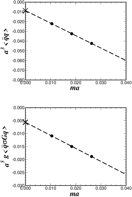
Figure 3: The bare condensates $a^{3}\langle\bar{q}q\rangle$ and $a^{5}g\langle\bar{q}\sigma_{\mu\nu}G_{\mu\nu}q\rangle$ plotted against the quark mass $ma$ at $\beta=6.0$. The dashed lines denote the best linear extrapolations, and the cross symbols correspond to the values in the chiral limit. The jackknife errors are hidden in the dots.

Figure 3 shows the values of the bare condensates $a^{3}\langle\bar{q}q\rangle$ and $a^{5}g\langle\bar{q}\sigma_{\mu\nu}G_{\mu\nu}q\rangle$ against the quark mass $ma$. We emphasize that the jackknife errors are almost negligible, due to the high statistics of $1600$ data for each quark mass. From figure 3, both $\langle\bar{q}q\rangle$ and $g\langle\bar{q}\sigma_{\mu\nu}G_{\mu\nu}q\rangle$ show a clear linear behavior against the quark mass $m$. This feature is also found for $\beta=5.7$ and $5.8$. Therefore, we fit the data with a linear function and determine the condensates in the chiral limit. The results are summarized in Tables  2, 3 and  4.

Table 2: The numerical results of $a^{3}\langle\bar{q}q\rangle$ and $a^{5}g\langle\bar{q}\sigma_{\mu\nu}G_{\mu\nu}q\rangle$ for various $ma$ in SU(3)_c lattice QCD with $\beta$=6.0 and $16^{4}$. The last column denotes their values in the chiral limit obtained by the linear chiral extrapolation.

	$ma=0.0263$	$ma=0.0184$	$ma=0.0105$	chiral limit
$a^{3}\langle\bar{q}q\rangle$	$-0.04240(16)$	$-0.03247(15)$	$-0.02212(16)$	$-0.00872(17)$
$a^{5}g\langle\bar{q}\sigma_{\mu\nu}G_{\mu\nu}q\rangle$	$-0.01882(15)$	$-0.01498(14)$	$-0.01088(14)$	$-0.00565(14)$

Table 3: The numerical results of $a^{3}\langle\bar{q}q\rangle$ and $a^{5}g\langle\bar{q}\sigma_{\mu\nu}G_{\mu\nu}q\rangle$ for various $ma$ in SU(3)_c lattice QCD with $\beta$=5.8 and $12^{4}$. The last column denotes their values in the chiral limit obtained by the linear chiral extrapolation.

	$ma=0.0368$	$ma=0.0258$	$ma=0.0147$	chiral limit
$a^{3}\langle\bar{q}q\rangle$	$-0.08031(35)$	$-0.06667(35)$	$-0.05159(36)$	$-0.03271(38)$
$a^{5}g\langle\bar{q}\sigma_{\mu\nu}G_{\mu\nu}q\rangle$	$-0.03883(32)$	$-0.03375(32)$	$-0.02783(31)$	$-0.02064(32)$

Table 4: The numerical results of $a^{3}\langle\bar{q}q\rangle$ and $a^{5}g\langle\bar{q}\sigma_{\mu\nu}G_{\mu\nu}q\rangle$ for various $ma$ in SU(3)_c lattice QCD with $\beta$=5.7 and $8^{4}$. The last column denotes their values in the chiral limit obtained by the linear chiral extrapolation.

	$ma=0.050$	$ma=0.035$	$ma=0.020$	chiral limit
$a^{3}\langle\bar{q}q\rangle$	$-0.12346(68)$	$-0.10788(73)$	$-0.09017(80)$	$-0.06833(90)$
$a^{5}g\langle\bar{q}\sigma_{\mu\nu}G_{\mu\nu}q\rangle$	$-0.06200(53)$	$-0.05695(56)$	$-0.05064(60)$	$-0.04327(66)$

III.2 Check on the systematic uncertainty

In this section, we check the reliability of our lattice QCD results. We first consider the finite volume artifact. As indicated by the Banks-Casher formula Banks ,

$$\lim_{m\rightarrow 0}\lim_{V\rightarrow\infty}\langle\bar{q}q\rangle = -\pi\frac{\rho(0)}{V},$$ (22)

for the spectral density $\rho(\lambda)$ of the Dirac operator, the total volume $V$ should be large enough before the quark mass goes to zero. In order to estimate this finite volume artifact, we carry out the same calculation imposing the periodic boundary condition on the Grassmann fields $\chi$ and $\bar{\chi}$, instead of the anti-periodic boundary condition, keeping the other parameters same. If the lattice total volume is too small, the quark propagates over the total volume, and the results would be sensitive to the boundary conditions. Thus, the difference will indicate ambiguity from the finite volume artifact.

Table 5: The lattice results of $a^{3}\langle\bar{q}q\rangle$ and $a^{5}g\langle\bar{q}\sigma_{\mu\nu}G_{\mu\nu}q\rangle$ with $\beta$=6.0 and $16^{4}$ in the case of the periodic boundary condition for the fermion field. This calculation is done for the check of the boundary effect and the finite volume artifact.

	$ma=0.0263$	$ma=0.0184$	$ma=0.0105$	chiral limit
$a^{3}\langle\bar{q}q\rangle$	$-0.04236(16)$	$-0.03240(16)$	$-0.02200(16)$	$-0.00854(17)$
$a^{5}g\langle\bar{q}\sigma_{\mu\nu}G_{\mu\nu}q\rangle$	$-0.01880(15)$	$-0.01493(14)$	$-0.01078(14)$	$-0.00551(14)$

We show in Table 5 the lattice results with the periodic boundary condition for $\beta=6.0$. Comparing with Table 2, one finds that the difference is only 1% level. The similar results are obtained for $\beta=5.7$ and $5.8$. Therefore, we conclude that the physical volume $V\sim(1.6\ {\rm fm})^{4}$ in our simulations is large enough to avoid the finite volume artifact.

We next consider the discretization error. As an advanced feature of the KS-fermion, the discretization error begins from ${\cal O}(a^{2})$ on the lattice spacing $a$. This is because ${\cal O}(a)$ errors cancel with each other when the average over the SU(4) flavor is taken. Therefore, there is no ${\cal O}(a)$ error originating from the quark propagator in Eqs. (13) and (14). On the other hand, there is an ambiguity coming from a particular choice of the gauge link ${\cal U}_{\mu,\nu}$ in Eq. (18), which is introduced to respect the gauge covariance. This ambiguity can be checked by changing the definition of $g\langle\bar{q}\sigma_{\mu\nu}G_{\mu\nu}q\rangle$, adopting a different path which connects the source point $(x+\rho)$ and the sink point $(x+\rho^{\prime})$ in Eq. (II). Specifically, instead of ${\cal U}_{\mu,\nu}$ in Eq. (18), we examine the other product $\tilde{\cal U}_{\mu,\nu}$ as

$$\tilde{\cal U}_{\pm\mu,\pm\nu}(x)\equiv U_{\pm\mu}(x)U_{\pm\nu}(x\pm\mu),$$ (23)

and thus define $g\langle\bar{q}\sigma_{\mu\nu}G_{\mu\nu}q\rangle$ by

$$a^{5}g\langle\bar{q}\sigma_{\mu\nu}G_{\mu\nu}q\rangle = -\frac{1}{2^{7}}\sum_{\mu>\nu}\sum_{\rho}{\rm Tr}\left[\ \tilde{\cal U}_{\pm\mu,\pm\nu}(x+\rho)\ \Gamma_{\rho^{\prime}}\Gamma_{\rho}^{\dagger}\ \langle\chi(x+\rho^{\prime})\bar{\chi}(x+\rho)\rangle\ \sigma_{\mu\nu}\ G_{\mu\nu}^{\rm lat}(x+\rho)\ \right],$$ (24)

where $\rho^{\prime}=\rho\pm\mu\pm\nu$ and the sign $\pm$ is taken as before. We perform the calculation for $\beta=5.7$ and $ma=0.050$. In this case, the lattice spacing $a$ is largest in our simulations, and therefore the discretization error is expected to be larger than the other cases for $\beta=5.8$ and $6.0$. At each gauge configuration, we check the difference of the results between the choice of Eq. (18) and Eq. (23). Since the typical difference is about 1%, we conclude that the discretization error is small enough, which confirms the reliability of our lattice results.

III.3 Determination of $m_{0}^{2}=g\langle\bar{q}\sigma_{\mu\nu}G_{\mu\nu}q\rangle/\langle\bar{q}q\rangle$

The values of the condensates in the continuum limit are to be obtained after the renormalization. To this end, the lattice perturbation theory has often been used, although it is afflicted with uncertainty originating from the non-perturbative effect. In principle, the non-perturbative renormalization scheme is desirable, which, however, requires a lot of computational power Martinelli . Therefore we seek for another way which can reduce this uncertainty. Here we provide the ratio $m_{0}^{2}\equiv g\langle\bar{q}\sigma_{\mu\nu}G_{\mu\nu}q\rangle/\langle\bar{q}q\rangle$, where some of the uncertainties are canceled with each other. In particular, this ratio is free from the uncertainty from the wave function renormalization of the quark. As a consequence, the results become more reliable with less uncertainties. In addition, the dependence of $m_{0}^{2}$ on the lattice spacing is weakened to $a^{2}$, while $\langle\bar{q}q\rangle$ and $g\langle\bar{q}\sigma_{\mu\nu}G_{\mu\nu}q\rangle$ are proportional to $a^{3}$ and $a^{5}$, respectively. We note that $m_{0}^{2}$ itself has the following physical meaning. In the QCD sum rule, $g\langle\bar{q}\sigma_{\mu\nu}G_{\mu\nu}q\rangle$ generally appears as the chiral variant term next to $\langle\bar{q}q\rangle$ in OPE. Therefore, $m_{0}^{2}$ is usually used without referring to the absolute value of $g\langle\bar{q}\sigma_{\mu\nu}G_{\mu\nu}q\rangle$ itself, and thus it represents the level of importance of $g\langle\bar{q}\sigma_{\mu\nu}G_{\mu\nu}q\rangle$ in OPE.

Now, we present the result of the ratio $m_{0}^{2}$ using the bare results in SU(3)_c lattice QCD. We adopt the results at $\beta=6.0$, since its lattice spacing is the finest in our calculations. We find in the chiral limit

$$m_{0}^{2}\equiv g\langle\bar{q}\sigma_{\mu\nu}G_{\mu\nu}q\rangle/\langle\bar{q}q\rangle\simeq 2.5\ {\rm GeV}^{2}\ (\beta=6.0),$$ (25)

at the lattice cutoff scale as $a^{-1}\simeq 2$ GeV. This large value of $m_{0}^{2}$ suggests the significance of the mixed condensate in OPE. Although we do not include renormalization effect, this result itself is determined very precisely.

IV Summary and Discussions

We have studied the quark-gluon mixed condensate $g\langle\bar{q}\sigma_{\mu\nu}G_{\mu\nu}q\rangle$ using SU(3)_c lattice QCD with the Kogut-Susskind fermion at the quenched level. First, we have emphasized that the mixed condensate is one of the key quantities in various quark hadron physics, especially in the baryon sector such as the $N$-$\Delta$ splitting. In spite of its importance, the lattice QCD studies of this quantity have been limited to only one preliminary study for 15 years. Recently, due to the progress in lattice QCD Monte Carlo calculations, it becomes possible to calculate this mixed condensate with much better statistics on a finer and larger lattice. For each quark mass of $m_{q}=21,36$ and $52$ MeV, we have generated 100 gauge configurations on the $16^{4},12^{4}$ and $8^{4}$ lattice with $\beta=6.0,5.8$ and $5.7$, respectively. We have performed the measurements of $g\langle\bar{q}\sigma_{\mu\nu}G_{\mu\nu}q\rangle$ as well as $\langle\bar{q}q\rangle$ at 16 physical space-time points in each gauge configuration. Using the 1600 data for each $m_{q}$, we have found $m_{0}^{2}\equiv g\langle\bar{q}\sigma_{\mu\nu}G_{\mu\nu}q\rangle/\langle\bar{q}q\rangle\simeq 2.5$ GeV² in the chiral limit at the lattice scale $a^{-1}\simeq 2$ GeV corresponding to $\beta=6.0$. We have checked that the systematic and statistical errors are almost negligible. Therefore, the value of $m_{0}^{2}$ at the lattice scale has been well determined in this calculation.

Finally, we compare our result with the standard value employed in the QCD sum rule. To this end, we change the renormalization point from $\mu\simeq\pi/a$ to $\mu\simeq 1$ GeV corresponding to the QCD sum rule. Following Ref. K&S , we first take the lattice results of the condensates as the starting point of the flow, then rescale the condensates using the anomalous dimensions evaluated in a perturbative manner. We have the following rescaled condensates as Narison2 ,

$$\langle\bar{q}q\rangle\Big{|}_{\mu} =\left(\frac{\alpha_{s}(\mu)}{\alpha_{s}(\pi/a)}\right)^{-4/b_{0}}\ \ \langle\bar{q}q\rangle\big{|}_{\pi/a},$$ (26)

$$g\langle\bar{q}\sigma_{\mu\nu}G_{\mu\nu}q\rangle\Big{|}_{\mu} =\left(\frac{\alpha_{s}(\mu)}{\alpha_{s}(\pi/a)}\right)^{2/(3b_{0})}\ \ g\langle\bar{q}\sigma_{\mu\nu}G_{\mu\nu}q\rangle\Big{|}_{\pi/a},$$ (27)

where we use the one-loop formula, $\alpha_{s}(\mu)=\frac{4\pi}{b_{0}\ln(\mu^{2}/\Lambda_{\rm QCD}^{2})}$ with $\Lambda_{\rm QCD}=200-300\mbox{MeV}$ and $b_{0}=(11/3)N_{c}-(2/3)N_{f}$. (The anomalous dimension given in Refs. Beneke ; Alad for $g\langle\bar{q}\sigma_{\mu\nu}G_{\mu\nu}q\rangle$ is different from Ref. Narison2 . However, this difference does not change our semi-quantitative analysis here.) For the case of the quenched lattice QCD, we adopt $N_{f}=0$. By using our bare lattice QCD results at $\beta=6.0$, we obtain $m_{0}^{2}\big{|}_{\mu}\equiv g\langle\bar{q}\sigma_{\mu\nu}G_{\mu\nu}q\rangle/\langle\bar{q}q\rangle\big{|}_{\mu}\sim 3.5-3.7\ {\rm GeV}^{2}$ at $\mu=1$GeV, from $\langle\bar{q}q\rangle\big{|}_{\mu}\sim-(0.0477-0.0506)\ {\rm GeV}^{3}=-(0.36-0.37{\rm GeV})^{3}$ and $g\langle\bar{q}\sigma_{\mu\nu}G_{\mu\nu}q\rangle\big{|}_{\mu}\sim-(0.176-0.177)\ {\rm GeV}^{5}$. Comparing with the standard value of $m_{0}^{2}=0.8\pm 0.2$ GeV² in the QCD sum rule, our calculation results in a rather large value. Note that the instanton model has made a slightly larger estimate as $m_{0}^{2}\simeq 1.4$ GeV² at $\mu\simeq 0.6$ GeV Polyakov . For a more definite determination of $m_{0}^{2}$, the renormalization procedure should be performed more carefully, which is also expected to improve the value of $\langle\bar{q}q\rangle$ simultaneously. In principle, the non-perturbative renormalization scheme is most desirable, which would, however, require a significant calculation cost Martinelli .

We again emphasize that the mixed condensate $g\langle\bar{q}\sigma_{\mu\nu}G_{\mu\nu}q\rangle$ plays very important roles in various contexts in quark hadron physics. Hence, it is preferable to perform further studies. In particular, the dynamical quark effects would be nontrivial, since the mixed condensate includes quark field. The thermal effects are also interesting in relation to chiral restoration, because the mixed condensate is another chiral order parameter. Actually, we are in progress with these two studies on the lattice DOIS:T . Considering the RHIC project, it becomes more and more important to understand the nature of finite temperature QCD. Therefore, it is quite desirable to determine thermal effects on the condensates with lattice QCD in understanding the finite temperature QCD.

References

• (1) M.A. Shifman, A.I. Vainshtein and V.I. Zakharov, Nucl. Phys. B 147, 385 (1979), ibid., 448 (1979).
• (2) L.J. Reinders, H. Rubinstein and S. Yazaki, Phys. Rep. 127, 1 (1985) and references therein.
• (3) B. L. Ioffe, Nucl. Phys. B188, 317 (1981), Erratum-ibid. B191, 591 (1981).
• (4) H.G. Dosch, M. Jamin, and S. Narison, Phys. Lett. B220, 251 (1989).
• (5) V.M. Belyaev and B.L. Ioffe, Sov. Phys. JETP 56, 493 (1982).
• (6) L.J. Reinders, H.R. Rubinstein, and S. Yazaki, Phys. Lett. B120, 209 (1983).
• (7) A.A. Ovchinnikov and A.A. Pivovarov, Sov. J. Nucl. Phys. 48, 721 (1988) (Yad. Fiz. 48, 1135 (1988)).
• (8) S. Narison, Phys. Lett. B210, 238 (1988).
• (9) H.G. Dosch, and S. Narison, Phys. Lett. B417, 173 (1998) and references therein.
• (10) J.I. Latorre, P. Pascual, and S. Narison, Z. Phys. C34, 347 (1987).
• (11) K.G. Wilson, Phys. Rev. D10, 2445 (1974).
• (12) M. Kremer and G. Schierholz, Phys. Lett. B194, 283 (1987).
• (13) H. J. Rothe, β€œLattice Gauge Theories” (World Scientific, 1997) 1.
• (14) T.T. Takahashi, H. Suganuma, Y. Nemoto and H. Matsufuru, Phys. Rev. D65, 114509 (2002).
• (15) T. Banks and A. Casher, Nucl. Phys. B169, 103 (1980).
• (16) G. Martinelli, C. Pittori, C.T. Sachrajda, M. Testa, and A. Vladikas, Nucl. Phys. B445, 81 (1995).
• (17) S. Narison and R. Tarrach, Phys. Lett. B125, 217 (1983).
• (18) K. Aladashvili and M. Margvelashvili, Phys. Lett. B372, 299 (1996).
• (19) M. Beneke and H.G. Dosch, Phys. Lett. B284, 116 (1992).
• (20) M.V. Polyakov and C. Weiss, Phys. Lett. B387, 841 (1996).
• (21) T. Doi, N. Ishii, M. Oka and H. Suganuma, Nucl. Phys. A (2003) in press, hep-lat/0212006; Proc. Int. Conf. on β€œQuark Confinement and the Hadron Spectrum V”, Italy, 2002, hep-lat/0212025 .