Residual mass effects in improved domain wall fermions

Abstract

In order to improve simulations with domain wall fermions (DWFs), it has been suggested to project out a number of low-lying eigenvalues of the 4-dimensional Dirac operator that generates the transfer matrix of DWF. We investigate how this projection method affects chiral properties of quenched DWF. In particular, we study the behaviour of the residual mass as a function of the size of the extra dimension.

1 Introduction

Domain wall fermions (DWFs) preserve chiral symmetry [1, 2, 3] when the lattice size in the 5th direction, $N_{s}$, is taken to infinity. A measure of chiral symmetry breaking is the residual mass $m_{\mathrm{res}}$. Even though the restoration of chiral symmetry is expected to be exponentially fast in $N_{s}$, in practice $m_{\mathrm{res}}$ decreases very slowly as first shown by CP-PACS [4, 5]. This is due to the existence of very small eigenvalues of the transfer matrix along the 5th direction. At large $N_{s}$ these eigenvalues determine the rate of the exponential decay. It is clear that any improvement of the chiral properties of DWF has to come from eliminating these low-lying eigenvalues.

One idea is to improve the gauge actions [4, 5, 6, 7]. However, besides the potential difficulties with unitarity violations and the sampling of topological charge sectors, this method does not solve completely the problem. In particular with the Iwasaki gauge action, the convergence rate also becomes slow at large $N_{s}$ [5] (see Fig. 2): very small eigenvalues of the transfer matrix, even though less frequently, also appear in this case. Using the DBW2 action seems to be much better in this respect [7], but it is unclear whether these small eigenvalues could eventually appear there, too, leading to similar problems.

Another method to eliminate the small eigenvalues is to project them out of the transfer matrix [8, 9]. In this contribution, we investigate the projection method based on Ref.[8], where the projection is performed on the transfer matrix itself. (In Ref.[9], the projection is operated only on a boundary term.) The aim of this paper is to investigate the effects of the projection method on the residual mass in the quenched configurations.

2 Domain wall fermions

Details of our notation can be found in Ref.[8], and we give only a brief summary below.

The 5D domain wall operator is defined as

$${\cal D}=\frac{1}{2}\left\{\gamma_{5}\left(\partial^{*}_{s}+\partial_{s}\right)-a_{5}\partial_{s}\partial_{s}\right\}+{\cal M}\quad,$$ (1)

where the operator ${\cal M}$ is obtained from the standard 4D Wilson–Dirac operator with negative mass (DW mass). Choosing open boundary conditions in the 5th dimension, chiral modes with opposite chiralities are localized on the 4D boundary plane at $s=1$ and $N_{s}$. The action of “quark fields”, which are constructed from the boundary fermions, is related to an effective 4D operator $D_{N_{s}}$, which satisfies

$$aD\equiv\lim_{N_{s}\rightarrow\infty}aD_{N_{s}}=1-\frac{A}{\sqrt{A^{\dagger}A}}\quad,$$ (2)

where

$$A=\frac{-a_{5}{\cal M}}{2+a_{5}{\cal M}}\quad.$$ (3)

The $D$ of eq.(2) satisfies the Ginsparg–Wilson relation and thus an exact lattice chiral symmetry.

In realistic simulations, for finite $N_{s}$, chiral symmetry is explicitly broken to a certain extent that can be quantified by the values of the so-called residual mass, which measures the anomalous term in the axial Ward–Takahashi identity [3]: $2J_{5q}(x)\equiv\nabla_{\mu}A_{\mu}(x)-2m_{f}P(x)$, where $A_{\mu}$ is the axial current and $P$ is the pseudoscalar density. The size of this extra chiral symmetry-breaking term can be described by the residual mass

$$m_{\mathrm{res}}=\lim_{t\rightarrow\infty}\frac{\sum_{\bf x}\langle J_{5q}(t,{\bf x})P(t,{\bf x})\rangle}{\sum_{\bf x}\langle P(t,{\bf x})P(t,{\bf x})\rangle}\quad.$$ (4)

2.1 Improvement of domain wall fermion

We employ a method to project out the small eigenvalue of $A^{\dagger}A$ [8]. The improved operator $\widehat{\cal{M}}$, instead of $\cal M$, satisfies the following relations in order that eqs.(2) and (3) hold;

$$\widehat{\cal M}^{\dagger}=\gamma_{5}\widehat{\cal M}\gamma_{5}\quad,\quad\det(2+a_{5}\widehat{\cal M})\neq 0\quad.$$ (5)

This is used to construct $\widehat{\cal M}$ in such a way that the very low eigenvalues of $A^{\dagger}A$ disappear, while keeping $D$ invariant. Following Ref.[8], the new operator ${\widehat{\cal M}}$ satisfying eq.(5) is given by the following expression;

$$\widehat{A}=\frac{-a_{5}\widehat{\cal M}}{2+a_{5}{\widehat{\cal M}}}=A+\sum_{k=1}^{r}(\widehat{\alpha}_{k}-\alpha_{k})\gamma_{5}v_{k}\otimes v_{k}^{\dagger}\,\,,$$ (6)

where $v_{k}$ is the eigenvector of $\gamma_{5}A$,

$$\gamma_{5}Av_{k}=\alpha_{k}v_{k}\,,\,\gamma_{5}\widehat{A}v_{k}=\widehat{\alpha}_{k}v_{k}\,,\,(v_{k},v_{l})=\delta_{kl}\,\,,$$ (7)

and $r$ is the number of eigenvalues projected out. Therefore an improved DWF operator can be obtained after substituting ${\cal M}$ in eq.(1) with $\widehat{\cal M}$ given by

$$a_{5}\widehat{\cal M}=a_{5}{\cal M}-\sum_{k,l=1}^{r}X_{kl}w_{k}\otimes w_{l}^{\dagger}\gamma_{5}\quad,$$ (8)

where $(X^{-1})_{kl}=2\delta_{kl}(\widehat{\alpha}_{k}-\alpha_{k})^{-1}+(v_{k},w_{l})$ and $w_{k}=(2+a_{5}{\cal M})\gamma_{5}v_{k}$.

3 Eigenvalues of matrix $A^{\dagger}A$

The eigenvalues of $A^{\dagger}A$ can be calculated by a straightforward generalization [8] of the Ritz functional method in Ref.[10]. We have calculated the convergence rate from eigenvalues of $A^{\dagger}A$ [8, 11] and the distributions of low-lying eigenvalues for various gauge actions [11].

4 Simulation of improved DWF

The values $\widehat{\alpha}_{k}$ can be chosen freely as long as $\widehat{\alpha}_{k}>\alpha_{k}$. This can be used to reduce the value of the residual mass. Here we use ${\widehat{\alpha}}_{k}=2{\rm sgn}(\alpha_{k})|\alpha_{l}|$ with $(\max\{k\};l)=(3;10)$ and $(10;10)$ in the plaquette gauge action. The notation in the figures is $\lambda_{\mathrm{proj}}=2\lambda_{l}=2|\alpha_{l}|$, then ${\widehat{\alpha}}_{k}={\rm sgn}(\alpha_{k})\lambda_{\mathrm{proj}}$.

For the Wilson gauge action we have chosen the gauge coupling to be $\beta=6.0$ ($a^{-1}\sim 2$ GeV) and the DW mass to be $m_{0}=1.8$. The lattice size is $12^{3}\times 24\times N_{s}$. This size is a little smaller than the ones used in simulations of the CP-PACS and RBC collaborations ($16^{3}\times 32\times N_{s}$); the value of the lattice spacing is, however, the same. The bare quark mass is always fixed to $m_{f}=0.02$.

In Fig.1, the quantity $\frac{\langle J_{5q}P\rangle}{\langle PP\rangle}$ without and with projection for $N_{s}=32$ and 48 is plotted. The number of projected modes is 0, 3 and 10. Note the large fluctuations of the residual mass when no projection is performed. As the number of eigenvalues projected out is increased, the determination of the residual mass is much more stable and cleaner.

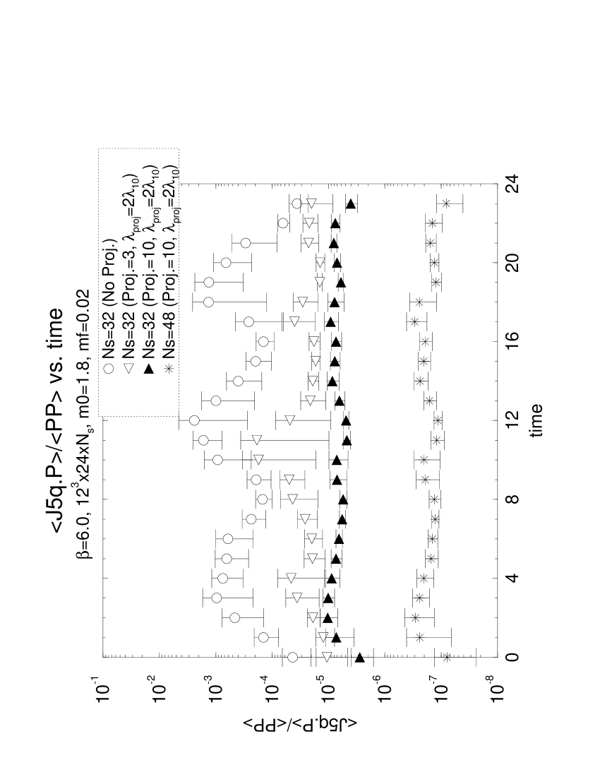
Figure 1: $\frac{\langle J_{5q}P\rangle}{\langle PP\rangle}$ without and with projection for $N_{s}=32$ and with projection for $N_{s}=48$. The fitting range for $m_{\mathrm{res}}$ is $4\leq t\leq 20$.

Figure 2 shows our main result: the comparison of the behaviour of the residual mass against $N_{s}$ for different improvement methods. The result at small $N_{s}$, for example $N_{s}=16$, reveals that the projection method does not show any effect. In the large-$N_{s}$ region, the effect of the projection of the low-lying eigenvalues on the residual mass is, however, remarkable. This is explained [5] by simple and qualitative arguments, as follows; $m_{\mathrm{res}}\sim\sum_{\alpha}e^{-\alpha N_{s}}\sim\int d\alpha\rho(\alpha)e^{-\alpha N_{s}}$, where $\alpha$ is the square root of eigenvalues of the operator $A^{\dagger}A$ and $\rho(\alpha)$ is the eigenvalue density, which grows with $\alpha$. In the contribution to the residual mass of each eigenvalue, there is a competition between the density function and the exponential suppression. Therefore, at large $N_{s}$, the low-lying eigenvalues dominate owing to the exponential suppression. At small $N_{s}$, however, not only low-lying but also bulk eigenvalues contribute to $m_{\mathrm{res}}$, owing to $\rho(\alpha)$.

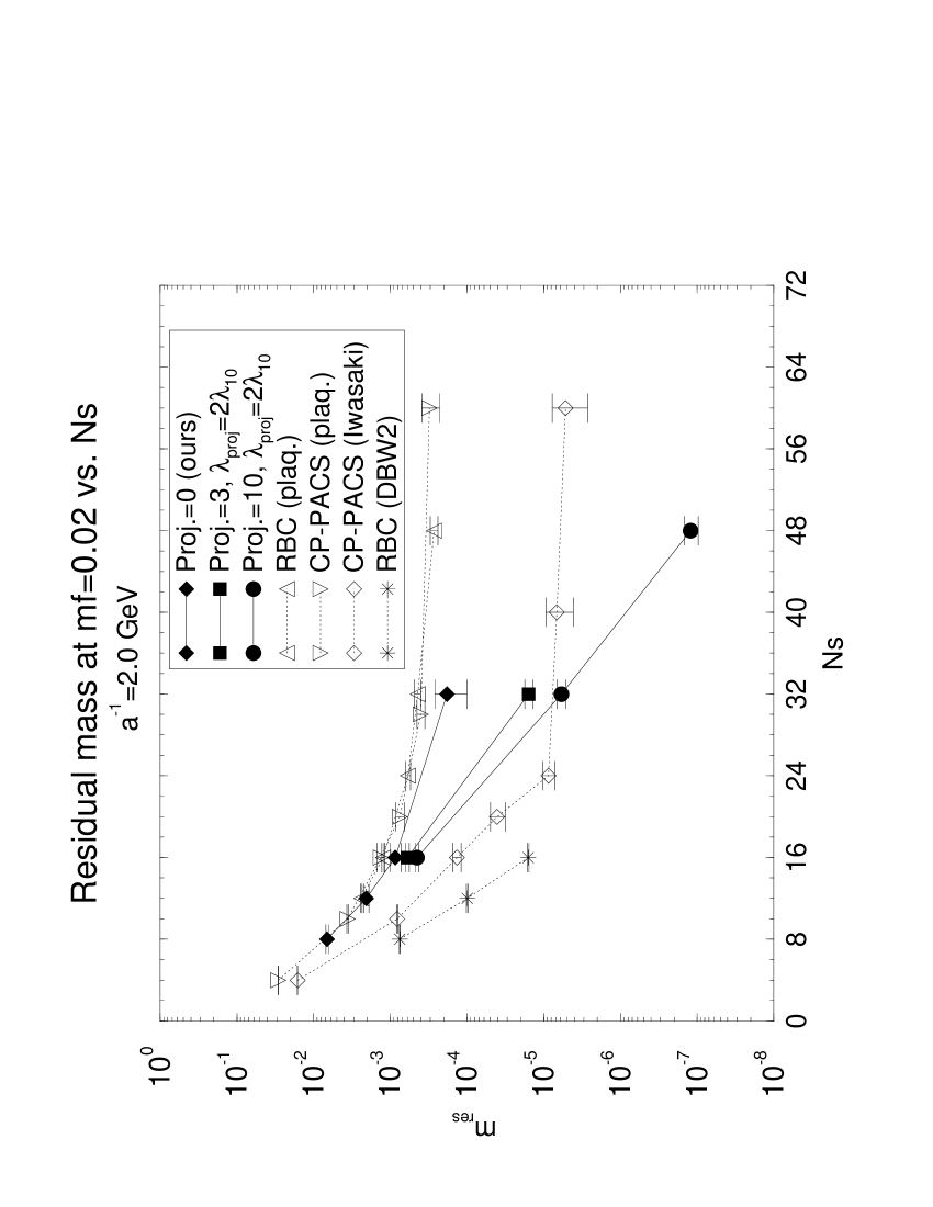
Figure 2: Residual mass as a function of $N_{s}$ with and without using the projection method. Filled symbols represent our data. We also add data from simulations of the CP-PACS and RBC collaborations for comparison. The lines are just to guide the eyes.

5 Summary

We have studied the residual mass effect of the projection method [8] on the restoration of chiral symmetry for quenched DWF. At large $N_{s}$, the low-lying eigenvalues of $A^{\dagger}A$ dominate the behaviour of the residual mass. Therefore the decay rate of the residual mass with $N_{s}$ can be simply controlled by the number of modes projected out. The residual mass for smaller $N_{s}$, however, is controlled by the low-lying and bulk eigenvalues. This is consistent with the arguments in the previous section [5]. Our numerical study shows that the projection method is superior to the improvement of the gauge action at large $N_{s}$.

We have also observed that the quantity $\langle J_{5q}P\rangle/\langle PP\rangle$ becomes much more stable after performing the projection, which may affect also other correlation functions to be stable and clean.

Since the projection method leads to a small numerical overhead, we conclude that using Wilson gauge action combined with the projection method is competitive with using improved gauge actions. To understand the projection method further, we are investigating the projection method with improved gauge actions [11].

References

- [1] D. Kaplan, Phys. Lett. B288 (1992) 342.
- [2] Y. Shamir, Nucl. Phys. B406 (1993) 90.
- [3] V. Furman and Y. Shamir, Nucl. Phys. B439 (1995) 54.
- [4] CP-PACS collaboration, Phys. Rev. D63 (2001) 114504.
- [5] CP-PACS collaboration, Nucl. Phys. B (Proc. Suppl.) 106 (2002) 718-720.
- [6] RBC collaboration, hep-lat/0007038.
- [7] RBC collaboration, Nucl. Phys. B (Proc. Suppl.) 106 (2002) 721-723.
-
[8]
P. Hernández, K. Jansen and M. Lüscher,
hep-lat/0007015. - [9] R. Edwards and U. Heller, Phys. Rev. D63 (2001) 094505.
- [10] B. Bunk, K. Jansen, M. Lüscher and H. Simma, DESY report (September 1994).
-
[11]
P. Hernández, K. Jansen and K.-I. Nagai,
in preparation.