Electric Polarizability of Hadrons

Abstract

The electric polarizability of a hadron allows an external electric field to shift the hadron mass. We try to calculate the electric polarizability for several hadrons from their quadratic response to the field at $a=0.17\,$fm using an improved gauge field and the clover quark action. Results are compared to experiment where available.

1 Introduction

The electric polarizability of a hadron characterizes the reaction of the quarks to an external electric field and can be measured by experiment (via Compton scattering) and on the lattice. Conceptually, an electric field will tend to separate charges in a hadron, thereby affecting the internal energy of the hadron and thus the mass. As in classical physics, the energy density goes as the square of the electric and magnetic fields:

$$\Delta m=-\frac{1}{2}\,\alpha E^{2}-\frac{1}{2}\,\beta B^{2}$$ (1)

where ${\alpha}$ $(\beta)$ is the electric (magnetic) polarizability that compares to experiment. See [1] for a calculation of the magnetic polarizability.

As is usual in lattice calculations, the mass of a hadron can be calculated from the exponential decay of a correlation function. By calculating the ratio of the correlation function in the field to that without the field, we have a ratio of exponentials that decays as a single exponential at the rate of the mass difference. Equation (1) implies that this mass difference (between in and out of the field) plotted versus the electric field will be parabolic with coefficient equal to minus half the polarizability. By averaging $\Delta m$ over the field, $E$, and its inverse, $-E$, we hope to minimize the linear term in the parabolic fit.

This calculation of the polarizabilities of several hadrons will follow the ideas discussed by Fiebig, et al. [2]; however, they used staggered fermions and we do not. Specifically, we include the static E-field on the links as a phase: (with fermion charge $q=Qe$)

$$e^{iaqA}=e^{i(a^{2}qE)(x_{4}/a)}=e^{i\eta\tau}\rightarrow(1+i\eta\tau)$$ (2)

Since the electric field is linearized in the continuum, we used the linearized form on the lattice. Fiebig, et al. found no significant difference between the exponential and linearized formats for similar electric field values. In addition, although the electric field breaks the isospin symmetry and allows the pion, a vector meson, to mix with glueballs, we ignore this effect in our calculation.

2 Lattice Details

This calculation uses the tadpole-improved clover quark action on a quenched $12^{3}\times 24$ lattice with $\beta=7.26$ ($a=0.17\,{\rm fm}$). The gauge field was thermalized to $10^{4}$ sweeps and then saved every 1000. We have 100 configurations, but only 17 were used in these preliminary results.

Including the static electric field as a phase on the links affects the Wilson term, but not the clover loops. In units of $10^{-3}e^{-1}a^{-2}$, the electric field took the values $-2.16$, $4.32$, $-8.64$, and $17.28$ via the parameter $\eta=a^{2}QeE$ in Eq. (2).

With $\kappa_{\rm cr}=0.1232(1)$, we used six values of $\kappa=0.1182$, $0.1194$, $0.1201$, $0.1209$, $0.1214$, and $0.1219$, which roughly correspond to $m_{q}\sim 200$, $150$, $120$, $90$, $70$, and $50$ MeV.

3 Results and Conclusion

The tightness of the parabola formed by graphing the mass shift of a particle versus the applied electric field will give the electric polarizability when fit with Eq. (1) at $B=0$.

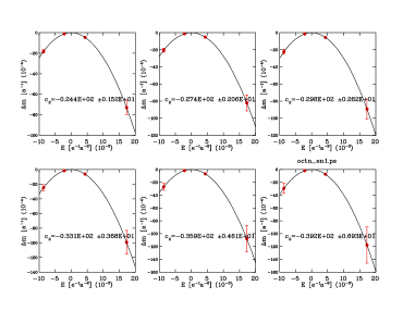
Figure 1: The neutron mass shift plotted versus electric field for the six $\kappa$ values given in the text.

The results for the neutron are shown in Fig. 1. The graphs are sorted by mass, large to small displayed from the upper-left across and down to the lower-right. The nice parabolic fit of Fig. 1 indicates that averaging over both directions of the field, $E$ and $-E$, has minimized any linear dependence. Similar graphs can be produced for the $\Delta^{0}$, $\pi^{0}$ and $\rho$ to varying degrees of confidence.

With more configurations, we will consider the chiral limit by combining the quadratic coefficient from these results into a plot of polarizability versus mass. Fig. 2 shows the neutron polarizability increasing in this limit.

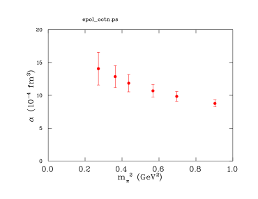
Figure 2: The polarizability of the neutron plotted versus $m_{\pi}^{2}$ as determined from the six graphs of Fig. 1.

With only 17 configurations, our preliminary result is not quite consistent with the average of the tabulate results, $10.4\times 10^{-4}\,{\rm fm^{3}}$.

Although $\chi$PT [3] predicts that $\alpha_{\pi}$ will be small and negative, $\approx-0.5\times 10^{-4}\,{\rm fm^{3}}$, Fig. 5 shows peculiarly large results.

Figure 3: The polarizability of the $\pi^{0}$ plotted versus $m_{\pi}^{2}$.

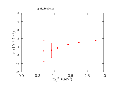
Figure 4: The polarizability of the $\Delta^{0}$ plotted versus $m_{\pi}^{2}$.

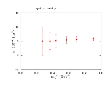
Figure 5: The polarizability of the $\rho^{0}$ plotted versus $m_{\pi}^{2}$.

The delta polarization seems to be dropping off in Fig. 5, and amidst large error-bars, the rho of Fig. 5 seems quite flat.

Table 1 lists the following subset of existing values for the neutron polarizability. There is by no means a consensus in the results.

Table 1: Current experimental values ([4, 5, 6, 7] with modifications by [8, 9]) and theoretical values (back to 2000) for the polarizability of the neutron. Several calculations are refinements to previous calculations. $\alpha_{n}$ is listed in units of $10^{-4}\,{\rm fm^{3}}$.

ref: method	$\alpha_{\rm n}$
[4]: Exp: Quasi-Free $\gamma d$	$10.7^{+3.3}_{-10.7}$
[5, 8]: Exp: $n$-208Pb	$12.6\pm 1.5\pm 2.0$
[6, 8]: Exp: $n$-208Pb	$0.6\pm 5$
[7]: Exp: uses [4]	$13.6^{+0.4}_{-6.0}$
[9]: claims [5, 8] is	$7-19$
[10]: Potential model	$9\pm 3$
[11]: Dressed K model	$12.7$
[12]: using [10]’s results	$12.5\pm 1.8^{+1.1}_{-0.6}\pm 1.1$
[13]: with [10]’s authors	$9.2\pm 2.2$

Experimentally, $\alpha_{n}$ is found through Compton scattering off of a deuteron and the polarizability of a proton must be included in the model. In this data, there are four experimental results, [4, 5, 6, 7]; but [7] incorporates [4]. L’vov [8] corrected the earlier values by adding $0.6\times 10^{-4}\,{\rm fm^{3}}$ to their results. The experiments measure $\alpha-\beta$ and the results are found using a sum rule that gives $\alpha+\beta$. The results are quite model-dependent, and even the experiments do not agree. We note that [9] claims [5, 8] miscalculated their errors. Further, [12] used [10]’s results to get a different number and then the authors of [10] joined others [13] to find a result close to their original value.

With consistent results for the neutron, we believe that finishing this calculation on the rest of our configurations will give results that can reliably be compared to the experimental results.

References

- [1] L. Zhou, F.X. Lee, W. Wilcox, J. Christensen, these proceedings.
- [2] H. R. Fiebig, W. Wilcox, R. M. Woloshyn, Nucl. Phys. B324 (1989) 47.
- [3] J. Portoles, M. R. Pennington, Second DAPHNE Physics Handbook 2* (1994) 579, [hep-ph/9407295v2].
- [4] K. W. Rose, et al., Nucl. Phys. A514 (1990) 621; Phys. Lett. B234 (1990) 460-464.
- [5] J. Schmiedmayer, P. Riehs, J. A. Harvey, N. W. Hill, Phys. Rev. Lett. 66 (1991) 1015.
- [6] L. Koester, et al., Phys. Rev. C51 (1995) 3363.
- [7] N. R. Kolb, et al., Phys. Rev. Lett. 85 (2000) 1388, [nucl-ex/0003002v3].
- [8] A. I. Lvov, Int. J. Mod. Phys. A8 (1993) 5267.
- [9] T. L. Enik, L. V. Mitsyna, V. G. Nikolenko, A. B. Popov, G. S. Samosvat, Phys. Atom. Nucl. 60 (1997) 567.
- [10] M. I. Levchuk, A. I. L’vov, Nucl. Phys. A674 (2000) 449, [nucl-th/9909066v2].
- [11] S. Kondratyuk, O. Scholten, Phys. Rev. C64 (2001) 024005, [nucl-th/0103006v2].
- [12] K. Kossert, et al., Phys. Rev. Lett. 88 (2002) 162301, [nucl-ex/0201015v2].
- [13] M. Lundin, et al. [nucl-ex/0204014v1].