The phase diagram of the three-dimensional $Z_{2}$ gauge Higgs system
at zero and finite temperature

Abstract

We study the effect of adding a matter field to the $\mathbb{Z}_{2}$ gauge model in three dimensions at zero and finite temperature. Up to a given value of the parameter regulating the coupling, the matter field produces a slight shift of the transition line without changing the universality class of the pure gauge theory, as seen by finite size scaling analysis or by comparison, in the finite temperature case, to exact formulas of conformal field theory. At zero temperature the critical line turns into a first-order transition. The fate of this kind of transition in the finite temperature case is discussed.

1 INTRODUCTION

The three-dimensional $\mathbb{Z}_{2}$ gauge Higgs system is perhaps the simplest example of a gauge theory coupled to a matter field. Its action can be written as

$$S=-\beta_{G}\sum_{\square\in\Lambda}U_{\square}-\beta_{I}\sum_{\langle xy\rangle}\sigma_{x}U_{xy}\sigma_{y}$$ (1)

where $U_{\square}=\prod_{\ell\,\in\square}U_{\ell}$, $U_{\ell}=\pm 1$, $\Lambda$ is a cubic lattice and $\sigma=\pm 1$ denotes the matter field. This model is self-dual under a Kramers-Wannier transformation:

$$Z(\beta_{G},\beta_{I})=\sum_{conf.}{\rm e}^{-S}\propto Z(\tilde{\beta}_{I},\tilde{\beta}_{G})~{},$$ (2)

with $\tilde{\beta}=-\log\sqrt{\tanh\beta}$. Its phase structure has been determined long ago [1] and it has been shown to be very similar to that of $SU(2)$ gauge system coupled to a matter field in the fundamental representation, but of course it is much simpler, moreover the coupling to the Ising matter can be now efficiently implemented by a non-local cluster algorithm [2] which leads to very accurate Monte Carlo (MC) simulations. Therefore it appears as an ideal laboratory to test new ideas on the confining-deconfining properties of coupled gauge models. Recently it has been used to study the phenomenon of string breaking [3, 4, 5] in order to probe a general mechanism proposed to explain why this phenomenon is not visible in the Wilson loops [6].

In this contribution we report an accurate analysis of the transition lines of this model at zero and at finite temperature.

At zero temperature we use the histogram method and the re-weighting techniques [8, 9, 10] to locate the first order transition line and the standard finite size scaling study of the continuous transitions, which turn out to be in the universality class of $3D$ Ising model. We find that the apparent triple point suggested by the old analysis based on the hysteresis cycles [1] is a finite size effect.

At finite temperature we argue that the matter field term in the action, for not too large values of $\beta_{I}$, is an irrelevant operator of the deconfining transition of the pure $\mathbb{Z}_{2}$ gauge theory, which is known to belong to the $2D$ Ising universality class. We support this conjecture by comparing the Polyakov correlator with the exact formula of spin-spin correlator in a finite box given by the underlying 2D conformal theory. This allows us to locate the transition lines in the plane $\beta_{G},\beta_{I}$ . For large enough $\beta_{I}$ the nature of the transitions changes and becomes strongly influenced by the boundary conditions.

2 ZERO TEMPERATURE

The problem of detecting a first order transition by MC simulations on a finite system of volume $V=L^{3}$ can be solved by computing the histogram of energy distribution $P(E,L)$ at a point $\beta_{G},\beta_{I}$ close to the transition line and then extrapolating the data to nearby values [8, 9, 10]

Figure 1: The double peak structure of the histogram of the link and the plaquette distribution near a first-order transition.

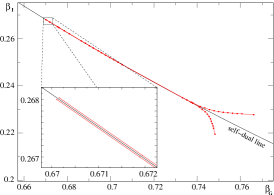
Figure 2: Location of the double peak in the L=18 lattice as a result of nine actual simulations corresponding to $1.2\,10^{7}$ MC steps.

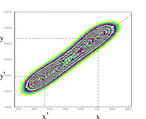
Figure 3: Contour plot of the double peak structure of Fig.(1) in the plaquette ($x$) and link ($y$) plane.

Figure 4: A typical plot of $W=-\log P(E,L)$ with $L=18$ on the self-dual line.

Figure 5: Finite size scaling behavior of the transition line near the bifurcation. The three curves are the fits to Eq.(7). At each value of $L$ the points are obtained by re-weighting the data of a single simulation.

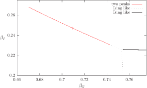
Figure 6: A schematic view of the phase diagram of the $\mathbb{Z}_{2}$ gauge Higgs model at zero temperature in the infinite volume limit. The cross indicates the point where the first-order transition has its maximal strength.

$$P(E,L)=\Omega(E,L)\frac{\exp{-\beta_{G}E}}{Z}~{}~{},$$ (3)

where $Z$ is the partition function and $\Omega(E,L)$ is the number of states of energy $E=-\sum_{\square}U_{\square}-\frac{\beta_{I}}{\beta_{G}}\sum_{\langle xy\rangle}\sigma_{x}U_{xy}\sigma_{y}$. In the vicinity of a first order transition it has a characteristic double peak structure as shown in the double histogram of the links and plaquettes of Fig.(1). A suitable re-weighting through Eq.(3) yields the line $\beta_{I}=f(\beta_{G},L)$ where the two peaks at $E_{1}(\beta_{G},\beta_{I},L)$ and $E_{2}(\beta_{G},\beta_{I},L)$ are of equal height. We located numerically this line for cubic lattices of sides ranging from $L=10$ to $L=30$. The autocorrelation times for larger lattices were too large in our canonical MC simulations. Perhaps more refined techniques such as multi-canonical algorithm [11] could reduce this correlation significantly. A typical plot of $\beta_{G}=f(\beta_{I},L)$ is reported in Fig.(2): it is formed by two dual lines which cross each other on a self-dual point. Above the crossing point the distance of these two curves from the self-dual line (SDL) decreases rapidly when $L$ increases and is already microscopic at $L=18$ (see the inset of Fig.(2)). If the system had a true triple point, one should see a triple peak near the crossing point, while we observe in all the cases a sharp double peak structure as represented in Fig.(1). Denoting by $(x,y)$ and $(x^{\prime},y^{\prime})$ the coordinates of the two peaks in the $(plaquette,link)$ plane (see Fig.(3)) it is easy to prove that, if two states coexist at a self-dual point, they are related, in the thermodynamic limit, by

$$x+y^{\prime}\,\sinh 2\beta_{I}=\cosh 2\beta_{I}$$ (4)

$$x^{\prime}+y\,\sinh 2\beta_{I}=\cosh 2\beta_{I}$$ (5)

which turn out to be approximately verified also in the finite lattices. It is worth observing that the presence of a double peak is not sufficient to assure a true first order transition. A useful quantity in this regard is the bulk free-energy barrier $\Delta F$ between the two coexisting states, defined by

$$\Delta F(L)=W(E_{m})-W(E_{1})~{},$$ (6)

where $W=-\log P(E,L)$ and $E_{m}((\beta_{G},\beta_{I},L)$ is the local maximum which separates the two dips at $E_{1}$ and $E_{2}$ when $W(E_{1})=W(E_{2})$, as shown in Fig.(4). At a continuous transition, $\Delta F(L)$ is independent of $L$ and at a first-order transition it increases monotonically with $L$. For large enough $L$ one has [12], for periodic boundary conditions, $\Delta F(L)\sim 2\sigma L^{2}$, where $\sigma$ is the interface tension. In our data at fixed $L$ $\Delta F$ is maximal at the crossing point. Extrapolating to large $L$ we locate the point where the first-order transition has its maximal strength at $\beta_{G}=0.708(2)$, $\beta_{I}=-\log(\tanh(\beta_{G}))/2$ and the corresponding interface tension is $2\sigma=.00108(9)$.

Using the behavior of $\Delta F(L)$ as a criterion for discriminating the order of the transition, we can prove the first-order nature only for a small interval around the crossing point. Near the bifurcation, where the transition lines go off the SDL, even if small lattices show still the double peak structure, the transition is second order. To extract an estimate for the infinite-volume transition line in this region, we tried the standard finite-size scaling form

$$\beta_{G}(L)=f(\beta_{I},\infty)-c(\beta_{I})\,L^{-\frac{1}{\nu}}~{},$$ (7)

which turns out to fit well the data, as Fig.(5) shows, using $\nu=0.63$, which is the value of the corresponding critical index of the $3D$ Ising universality class. The resulting phase diagram in the thermodynamic limit is reported in Fig.(6).

3 FINITE TEMPERATURE

The universality class of a continuous deconfining transition of a pure gauge theory in $D$ dimensions is well understood in terms of the Svetitsky and Yaffe (SY) conjecture [13]: it coincides with that of the spin model in $D-1$ dimensions with a global symmetry coinciding with the center $C(G)$ of the gauge group. What is the effect of adding matter to a pure gauge system? there is no general answer. Even when the matter can be treated as a ’small’ perturbation ( using for instance the inverse mass $1/m$ as a perturbing parameter), it does not change the nature of the transition only if it is an irrelevant operator.

At first sight one is tempted to conclude that the matter acts always as a relevant operator, since it breaks explicitly the global center symmetry of the pure gauge theory at finite temperature, which is the hart of the SY conjecture.

In the model at hand, when the coupling $\beta_{I}$ of the matter is small enough, it is easy to show that this is not actually the case: the addition of the matter does not modify the universality class of the deconfining transition both at zero and at finite temperature. The argument goes as follows. Performing a duality transformation as defined in Eq.(2), when $\tilde{\beta}_{I}\to\infty$ we recover the usual 3D Ising model. For large $\tilde{\beta}_{I}$ it is possible to do a perturbation expansion in ${\rm e}^{-\tilde{\beta}_{I}}$. The first order correction is due to a single anti-ferromagnetic link, and the corresponding change in the free energy is proportional to ${\rm e}^{-4\tilde{\beta}_{I}}\langle\sum_{\langle xy\rangle}{\rm e}^{-2\tilde{\beta}_{G}\sigma_{x}\sigma_{y}}\rangle$. Near the critical point, this may be expanded in a sum of scaling operators all of which will be even under spin reversal. The dominant term is therefore proportional to the energy operator of the unperturbed Ising model, both at zero and at finite $T$. Therefore the only effect is that of a slight shift of the transition line, without changing the universal critical properties. So, in a sense, the matter field acts as an irrelevant perturbation of the universality class of the pure gauge theory. In order to extend this property to larger values of $\beta_{I}$ we have to resort to numerical work.

At finite $T$, where the deconfining transition is known to be well described by the $2D$ Ising universality class, we can support this property even at larger values of $\beta_{I}$ by accurate numerical tests of comparison with the exact finite size formulas dictated by the $2D$ conformal field theory.

At $\beta_{I}=0$, $N_{t}=6=1/T_{c}$ the deconfining transition is estimated to be at $\beta_{G}=0.746035$ [14]. Here the Polyakov loop correlators, according to the SY conjecture combined with the universal finite size effects dictated by the 2d conformal field theory, should be given by [15]

$$\langle L(0)L(\vec{x})\rangle\propto\frac{\sum_{\nu=1}^{4}|\theta_{\nu}(\frac{1}{2}z,\tau)|\left|\frac{\theta_{1}^{\prime}(0,\tau)}{\theta_{1}(z,\tau)}\right|}{\sum_{\nu=2}^{4}|\theta_{\nu}(0,\tau)|},$$ (8)

where $\hat{t}$ is the temporal direction, $L(\vec{x})=\prod_{n=1,\dots N_{t}}U_{\vec{x}+(n-1)\hat{t},\vec{x}+n\hat{t}}~{}$ is the Polyakov loop along $\hat{t}$ and $\theta_{\nu}(z,\tau)$ denotes the Jacobi theta functions of argument $z$ and modulus $\tau=i\frac{N_{y}}{N_{x}}\;$; a point $\vec{x}=(x_{1},x_{2})$ in the spatial plane is mapped to a complex number through $z=x_{1}+\tau x_{2}$. Note that $\langle L(0)L(\vec{x})\rangle\sim_{\vec{x}\to 0}\frac{1}{|\vec{x}|^{\frac{1}{4}}}~{},$ as expected at the critical point in the infinite volume limit.

If the matter field behaves as an irrelevant perturbation, this property should be valid even at $\beta_{I}>0$ at an appropriate value of $\beta_{G}(\beta_{I})$. This has been checked accurately on large lattices at $N_{t}=6$ and $20\leq N_{x},N_{y}\leq 160$.

A typical fit is reported in Fig.(7). Note that Eq.(8), being a formula derived in the context of the conformal field theory, is valid only in the continuum limit, so at short distance it is expected that Polyakov loop correlators may be affected by lattice artifacts. Our data suggest that the value predicted by the continuum limit is reached already at distances of $\sim$ 3 lattice spacings. Finite-size effects at criticality are rather strong due to scale invariance, and nontrivial. Therefore they are ideally suited to compare theoretical predictions with MC simulations. In particular Eq.(8) produces strong, universal shape effects through the modulus $\tau$, which takes into account the asymmetry of the lattice. A fit of the Polyakov correlators in an asymmetric lattice is reported in Fig.(8). Similar shape effects in the pure $\mathbb{Z}_{2}$ gauge theory at criticality where already observed in Ref. [16].

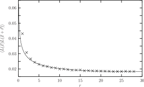
Figure 7: The Polyakov loop correlator at $\beta_{G}=0.7445,~{}\beta_{I}=0.17$ in a lattice of size $6\times 55\times 55$ compared with the critical 2D spin spin Ising correlator in a square box.

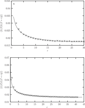
Figure 8: Shape effects on the Polyakov loop correlator: same as Fig.(7) with an asymmetric lattice of size $6\times 55\times 80$. In the two figures the correlator is taken along the two different coordinate axes.

We used the goodness of the data fits to Eq.(8) as a criterion to locate the transition line $\beta_{G}=f(\beta_{I})$ in the plane $\beta_{G},\beta_{I}$ below the SDL. The Kramers- Wannier transformation generates another critical line which is the dual $\tilde{\beta}_{I}=\tilde{f}(\tilde{\beta}_{G})$ of the previous line (see Fig.(9)). In the limit $\beta_{I}\to 0$ Eq.(2) yields $Z(\beta_{G},0)\propto\sum_{x,y,z}Z_{xyz}^{I}(\tilde{\beta}_{G})$ where $x,y,z$ denote periodic or anti-periodic boundary conditions (BC) in the 3 directions, and $Z_{xyz}^{I}$ is the usual Ising partition function. Anti-periodic BC are implemented by closed surfaces of anti-ferromagnetic links wrapped around the periodic directions.

When $\beta_{I}>0$ the sign of the links and consequently the BC become dynamical degrees of freedom, however

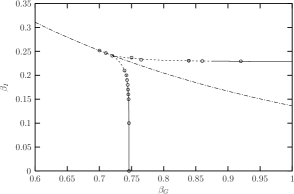
Figure 9: The phase diagram at finite temperature. The points below the SDL are obtained through comparison with Eq.(8). The points above are obtained by comparison with the critical partition function of $2D$ Ising model, as explained in Ref.[14].

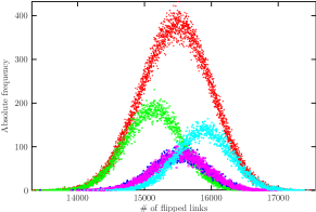
Figure 10: The histogram of the link distribution (highest curve) is separated into the contributions associated to different BC on the transition line near $\beta_{G}=0.86~{}$.

local updating algorithms on the critical line do not mix periodic and anti-periodic BC. Therefore the system behaves near the transition line above the SDL as a pure $2D$ critical Ising model. In the Fortuin Kasteleyn (FK) random cluster description we can indirectly evaluate the status of the BC by looking for the FK clusters with a linkage along the periodic directions. Transitions between periodic and anti-periodic BC are possible for not too large values of $\beta_{G}$. It turns out that when these kinds of transitions become statistically relevant, the nature of the transition line seems modified. In particular, the agreement of the dual transition below the SDL worsens and the expectation value of the link on the transition line above the SDL is somewhat influenced by the BC: even if the histogram of the distribution of the link (or the plaquette) variable does not show any macroscopic double peak structure, we can separate this distribution in various sets, according to the linking properties of the largest FK cluster, which gives an indirect information on the BC of the underlying Ising model. The result of this separation is reported in Fig.(10), which seems to indicate a very week first-order transition driven by the BC.

References

- [1] G.Jogeward, J.Stack, Phys.Rev. D21 (1980) 3360.
- [2] R.H. Swendsen and J.-S. Wang, Phys. Rev. Lett. 58, 86 (1987).
- [3] F. Gliozzi, Nucl. Phys. Proc. Suppl. 94 (2001) 550 [arXiv:hep-lat/0010084].
- [4] F. Gliozzi and A. Rago, [arXiv:hep-lat/0110064].
- [5] F. Gliozzi and A. Rago, [arXiv:hep-lat/0206017].
- [6] F. Gliozzi and P. Provero, Nucl. Phys. B 556 (1999) 76 [arXiv:hep-lat/9903013].
- [7] F. Gliozzi and P. Provero, Nucl. Phys. Proc. Suppl. 83 (2000) 461 [arXiv:hep-lat/9907023].
- [8] M. Falcioni, E. Marinari, M.L. Paciello, G.Parisi and B. Taglienti, Phys. Lett. 108B, 331 (1982)
- [9] E. Marinari, Nucl. Phys. B235 [FS11], 123 (1984).
- [10] A.M. Ferrenberg and R.H. Swendsen, Phys. Rev. Lett. 61, 2635 (1988).
- [11] B.A. Berg and Y. Neuhaus, Phys. Lett. B267, 249 (1991).
- [12] K. Binder, Phys. Rev. A25, 1699 (1982); J. Lee and J.M. Kosterlitz, Phys. Rev. Lett. 65 , 137 (1990).
- [13] B. Svetitsky and L. G. Yaffe, Nucl. Phys. B 210 (1982) 423.
- [14] M. Caselle and M. Hasenbusch, Nucl. Phys. B 470 (1996) 435 [arXiv:hep-lat/9511015].
- [15] P. Di Francesco, H. Saleur and J. B. Zuber, Nucl. Phys. B 290 (1987) 527.
- [16] F. Gliozzi and P. Provero, Phys. Rev. D 56 (1997) 1131 [arXiv:hep-lat/9701014].