Dynamical fermions on anisotropic lattices

Abstract

We report on our study of two-flavor full QCD on anisotropic lattices using $O(a)$-improved Wilson quarks coupled with an RG-improved glue. The bare gauge and quark anisotropies corresponding to the renormalized anisotropy $\xi=a_{s}/a_{t}=2$ are determined as functions of $\beta$ and $\kappa$, using the Wilson loop and the meson dispersion relation at several lattice cutoffs and quark masses.

1 Introduction

Study of quark gluon plasma using finite-temperature lattice QCD has seen a remarkable progress over the last decade. The equation of state (EOS) is one of the most studied topics, for which many calculations have been reported and have made clear the effects of dynamical quarks [1]. However, most studies on EOS in full QCD are made for the temporal lattice size of $N_{t}=4$ or $6$, and a reliable continuum extrapolation of EOS is prevented by large scale violation present for small $N_{t}$.

Recently, the CP-PACS Collaboration proposed the use of anisotropic lattice for calculations of EOS. This proposal was tested for the pure gluon system [2], for which a well-controlled continuum extrapolation of EOS was performed for the first time.

We wish to extend the use of anisotropic lattice to calculations of EOS for full QCD. This requires a tuning of the bare gauge and quark anisotropy parameters which corresponds to a given value of the anisotropy. In this paper we report results of such a tuning.

2 Lattice action

We adopt an O(a)-improved Wilson quark action coupled with an RG-improved action for gluons. This combination of actions has been adopted in a series of systematic investigations at $T=0$ [4]. It also shows better scaling properties in finite-temperature QCD, e.g., the expected O(4) scaling is observed around $T_{c}$ [3].

Here, we extend the study to anisotropic lattices. We focus on the anisotropy $\xi=a_{s}/a_{t}=2$, where $a_{s}$ and $a_{t}$ are the spatial and temporal lattice spacings, respectively. This choice of $\xi$ is based on a study of efficiency in calculations of EOS as described in our previous study in quenched QCD [2].

We consider the following gauge action which includes plaquette, $P_{\mu\nu}(x)$, and rectangle loop, $R_{\mu\nu}(x)$:

$$S_{G}=$$ (1)

$$\beta\{\gamma_{G}^{-1}\sum_{x,i>j}(c_{0}^{s}P_{ij}(x)+c_{1}^{s}\{R_{ij}(x)+R_{ji}(x)\})$$

$$+\gamma_{G}\sum_{x,k}(c_{0}^{t}P_{k4}(x)+c_{1}^{t}R_{k4}(x)+c_{2}^{t}R_{4k}(x))\},$$

where $c_{0}^{s}+8c_{1}^{s}=1$ and $c_{0}^{t}+4(c_{1}^{t}+c_{2}^{t})=1$. Carrying out the RG improvement program of Ref. [5] on this action, we find that a simple choice $c_{1}^{s}=c_{1}^{t}=c_{2}^{t}=-0.331$, which is the same as for the isotropic case, sufficiently improves the theory for small anisotropy $\xi\approx 1-4$ [6].

The quark action we study is as follows [7].

$$S_{F}=\sum_{x,y}\bar{q}(x)K(x,y)q(y),$$ (2)

$$K(x,y)=\delta_{x,y}-\kappa_{t}\{(1-\gamma_{4})U_{4}(x)\delta_{x+\hat{4},y}$$

$$+(1+\gamma_{4})U^{\dagger}_{4}(x-\hat{4})\delta_{x-\hat{4},y}\}$$

$$-\kappa_{s}\sum_{i}\{(r-\gamma_{i})U_{i}(x)\delta_{x+\hat{i},y}$$

$$+(r+\gamma_{i})U^{\dagger}_{i}(x-\hat{i})\delta_{x-\hat{i},y}\}$$

$$-(\kappa_{s}c_{t}\sum_{i}\sigma_{4i}F_{4i}(x)+r\kappa_{s}c_{s}\sum_{i>j}\sigma_{ij}F_{ij}(x))\delta_{x,y}.$$ (3)

The bare anisotropy $\gamma_{F}$ of the fermion field is defined by the ratio of the spatial and the temporal hopping parameters, $\kappa_{t}=\gamma_{F}\kappa_{s}$. We set the Wilson parameter to be $r=1/\xi$ [7]. The hopping parameters are related to the bare quark mass as $\kappa_{s}=1/[2(m_{q}+\gamma_{F}+3r)]$. We also define $\kappa$ by $1/\kappa=1/\kappa_{s}-2(\gamma_{F}+3r-4)$. This parameter plays the same role as $\kappa$ on the isotropic lattice. For free fermion, equating the rest and the kinetic masses leads to $\gamma_{F}^{-1}=\xi^{-1}(1+m_{q}^{2}/3)$ when $r=1/\xi$ [9].

For the field strength $F_{\mu\nu}$, we use the standard clover-leaf definition. At the tree level, the coefficients of the clover terms, $c_{s}$ and $c_{t}$, are unity. We incorporate the mean-field improvement, $U_{i}\rightarrow U_{i}/u_{0s}$ ($i=$1,2,3) and $U_{4}\rightarrow U_{4}/u_{0t}$, with the spatial mean-field factor defined with the plaquette in 1-loop perturbation theory $u_{0s}=(1-1.154/\beta)^{1/4}$, and $u_{0t}=1$ for the temporal mean-field.

3 Calibration procedure

To realize a consistent anisotropy, the bare anisotropy parameters $\gamma_{F}$ and $\gamma_{G}$ for fermion and gauge fields have to be calibrated, such that the anisotropy $\xi_{F}$ calculated in the fermionic sector coincides with $\xi_{G}$ calculated in the gluonic sector.

We perform this calibration as follows. Calculating $(\xi_{F},\xi_{G})$ for some parameter sets of $(\gamma_{F},\gamma_{G})$ at a fixed $\kappa$ and $\beta$, we make a fit of results with linear functions of $\gamma_{F}$ and $\gamma_{G}$, and locate the point satisfying $\xi_{F}=\xi_{G}=\xi$, where $\xi=2$ in our case. This point is denoted as $\gamma_{F}^{*}$ and $\gamma_{G}^{*}$, which are functions of $\beta$ and $\kappa$.

For the determination of $\xi_{G}$, we adopt Klassen’s method [8] of matching the Wilson loop ratios according to

$$\frac{W_{ss}(x,y)}{W_{ss}(x+1,y)}=\frac{W_{st}(x,t)}{W_{st}(x+1,t)},~{}~{}~{}~{}t=\xi_{G}y$$ (4)

where $W_{ss}(x,y)$ and $W_{st}(x,t)$ are spatial-spatial and spatial-temporal Wilson loop, respectively.

For $\xi_{F}$ we use the relativistic dispersion relation of mesons, and demand

$$E(\vec{p})^{2}=m^{2}+\frac{\vec{p}^{2}}{\xi_{F}^{2}}+O(\vec{p^{4}}),$$ (5)

where $E$ and $m$ are in units of $a_{t}$, while the spatial momentum $\vec{p}$ is in units of $a_{s}$. The latter is defined with $\vec{p}=2\pi\vec{n}/L_{s}$, $\vec{n}=(0,0,0),$ $(1,0,0)$ and its permutations. We evaluate $\xi_{F}$ using either pseudoscalar or vector mesons. The results are referred to as $\gamma_{F}^{*}(PS)$ and $\gamma_{F}^{*}(V)$ (and also $\gamma_{G}^{*}(PS)$ and $\gamma_{G}^{*}(V)$) for the calibrated bare anisotropies.

4 Simulation details

Simulations are made with the HMC algorithm for two flavors of degenerate quarks, using an even-odd preconditioned BiCGStab quark solver. The calibration is performed at $\beta=1.8,1.9$ and $2.0$ on a $8^{3}\times 24,8^{3}\times 24$ and $10^{3}\times 30$ lattice, respectively. Six values of $\kappa$ are used at each $\beta$ corresponding to $m_{PS}/m_{V}\simeq 0.6,0.7,0.8,0.85,0.9$ and $0.92$. Measurements are performed at every 5 trajectories up to 1000 – 1700 trajectories after 300 thermalization trajectiries. Errors are estimated by the jackknife method with bins of 50 trajectories, and error propagation is used in the fitting to $\xi=2$.

If the lattice scale is estimated from the Sommer scale $r_{0}=0.5$fm, the typical lattice size in the spatial direction is about 2.0 fm (2.3 fm) at $\beta=1.9,2.0$ ($\beta=1.8$) for $m_{PS}/m_{V}\simeq 0.8$.

5 Calibration results

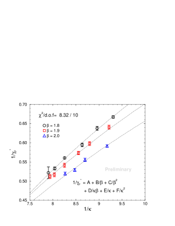
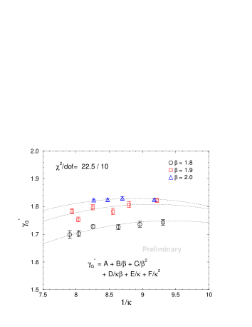
Figure 1: $1/\kappa$ dependence of calibration results at each $\beta$

Figure 1 shows the results for $\gamma_{G}^{*}$ and $1/\gamma_{F}^{*}$ as a function of $1/\kappa$ at each $\beta$. Unlike the case of quenched calculation [9], where $1/\gamma_{F}^{*}$ shows no linear terms in $m_{q}$, linear terms are important in full QCD even with the choice $r=1/\xi$. Therefore the results are fitted with a general quadratic function of $1/\beta$ and $1/\kappa$, $f(\beta,\kappa)=A+B/\beta+C/\beta^{2}+D/\beta\kappa+E/\kappa+F/\kappa^{2}$.

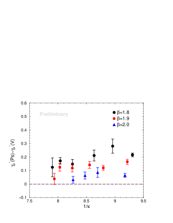
Figure 2: Difference between pseudoscalar and vector in determination of $\xi_{F}$

Figure 2 represents the difference between $\gamma_{F}^{*}(PS)$ and $\gamma_{F}^{*}(V)$. Non-vanishing values of this quantity represnets an $O(\alpha a)$ lattice artifacts for our action choice. We confirm that the difference tends to zero ( less than 5 % for $\beta\geq 2.0$) as $\beta$ is increased. We plan to use this difference to estimate systematic errors in continuum extrapolations.

An extension of the present calibration to the region of weaker coupling (larger $\beta$) is under way.

This work is supported in part by the Large-Scale Numerical Simulation Project of the Science Information Processing Center (S.I.P.C) of University of Tsukuba and by the Grants-in-Aid for Scientific Research by the ministry of Education (No.12304011, 12640253, 12740133, 13640259, 13640260, 13135204, 14046202, 11640294). The simulations are carried out on Fujitsu VPP5000 of S.I.P.C.

References

- [1] See e.g. S. Ejiri, Nucl. Phys. B(Proc.Suppl.)94 (2001) 16.
- [2] Y. Namekawa et al. (CP-PACS Collaboration), Phys. Rev. D64 (2001) 074507.
- [3] A. Ali Khan et al. (CP-PACS Collaboration), Phys. Rev. D63 (2000) 034502.
- [4] A. Ali Khan et al. (CP-PACS Collaboration), Phys. Rev. D65 (2002) 054505.
- [5] Y. Iwasaki, Nucl. Phys. B258 (1985) 141; Univ. of Tsukuba Report No. UTHEP-118 (1983).
- [6] S. Ejiri, K. Kanaya, Y. Namekawa and T. Umeda, in preparation.
- [7] J. Harada et al., Phys. Rev. D64 (2001) 074501.
- [8] T. R. Klassen, Nucl. Phys. B533 (1998) 557.
- [9] H. Matsufuru, T. Onogi and T. Umeda Phys. Rev. D64 (2001) 114503.