Unquenched domain wall quarks with TSMB

Abstract

The numerical simulation of domain wall quarks with the two-step multi-boson (TSMB) algorithm is investigated. Tests are performed on a $8^{3}\cdot 4$ lattice with $N_{f}=2$ quark flavours.

1 INTRODUCTION

Lattice actions with improved chiral properties offer the perspective of QCD simulations with a better control of chiral symmetry at non-zero lattice spacings. A prototype is the domain wall fermion action [1, 2, 3] defined on a five dimensional hypercubic lattice. Following Shamir’s formulation [3], the light chiral fermion modes are located on two boundaries of the fifth dimension. The price of the chiral symmetry at non-zero lattice spacing is the extra dimension enlarging the number of degrees of freedom. From a technical point of view this means that the extensions of the fermion matrix are larger and therefore the numerical simulations are slower.

It is an interesting question how much the computation speed decreases compared to, say, Wilson fermions. Since the good chiral properties of domain wall fermions develop only sufficiently close to the continuum limit, the performance studies have to be finally performed on large lattices. A comparison can only be conclusive if the autocorrelations of important physical quantities are also determined – a difficult task requiring a substantial amount of computer time.

A first step towards the effective simulation of domain wall quarks is to identify possible simulation algorithms which have the potential of being applicable in simulations with small quark masses and in large physical volumes. The two-step multi-boson algorithm (TSMB) [4]-[7] has been succesfully tested in this respect in case of the Wilson quark action [8, 9]. The application of TSMB for domain wall quarks has been recently considered in [10]. Here we report on some further tests along these lines.

2 ACTION AND ALGORITHM

The lattice action for domain wall quarks can be introduced as

$$S=S_{G}[U]+S_{F}[\overline{\Psi},\Psi,U]+S_{PV}[\Phi^{\dagger},\Phi,U]\ .$$ (1)

Here $S_{G}$ denotes the pure gauge-field part depending on the gauge field $U$, $S_{F}$ is the fermionic part with the Grassmannian quark fields $\Psi,\overline{\Psi}$ and $S_{PV}$ depends on the bosonic Pauli-Villars field $\Phi$ which subtracts the heavy fermion modes – as introduced in [11].

The fermion action $S_{F}$ is defined by

$$S_{F}=\sum_{x,s;\,x^{\prime},s^{\prime}}\overline{\Psi}(x^{\prime},s^{\prime})D_{F}(x^{\prime},s^{\prime};\,x,s)\Psi(x,s)\ .$$ (2)

The four-dimensional space-time coordinates are denoted by $x,x^{\prime}$ and the fifth coordinates are $s,s^{\prime}$. The domain wall fermion matrix $D_{F}$ is constructed from the standard four-dimensional Wilson fermion matrix

$$D(x^{\prime},x)=\delta_{x^{\prime}x}\;(4-am_{0})$$

$$-\frac{1}{2}\sum_{\mu=1}^{4}\raisebox{-1.29167pt}{\mbox{\LARGE$\left[\right.$}}\delta_{x^{\prime},x+\hat{\mu}}(1+\gamma_{\mu})U_{x\mu}$$

$$+\;\delta_{x^{\prime}+\hat{\mu},x}(1-\gamma_{\mu})U^{\dagger}_{x^{\prime}\mu}\raisebox{-1.29167pt}{\mbox{\LARGE$\left.\right]$}}\ .$$ (3)

The notations are standard: $a$ is the (four-dimensional) lattice spacing and $\hat{\mu}$ denotes the unit vector in direction $\mu$. The bare mass $-m_{0}$ is chosen to be negative and should be tuned properly for producing the light boundary fermion state. The non-zero matrix elements of the domain wall fermion matrix are:

$$(D_{F})_{s,s}=\sigma+D\ ,\;(D_{F})_{s,s+1}=-\sigma P_{L}\ ,$$

$$(D_{F})_{s+1,s}=-\sigma P_{R}\ ,\;(D_{F})_{1,N_{s}}=am_{f}P_{R}\ ,$$

$$(D_{F})_{N_{s},1}=am_{f}P_{L}\ .$$ (4)

Here $m_{f}$ denotes the bare fermion mass of the light boundary fermion, $N_{s}$ is the lattice extension in the fifth dimension, $P_{R}=\frac{1}{2}(1+\gamma_{5}),\;P_{L}=\frac{1}{2}(1-\gamma_{5})$ are chiral projectors and $\sigma\equiv a/a_{s}$ determines the lattice spacing in the fifth dimension $a_{s}$ relative to $a$.

The TSMB algorithm is based on the hermitean domain wall fermion matrix

$$\tilde{D}_{F}\equiv\gamma_{5}R_{5}\,D_{F}$$ (5)

where the reflection in the fifth dimension is defined as $(R_{5})_{s^{\prime},s}\equiv\delta_{s^{\prime},N_{s}+1-s}\;(1\leq s,s^{\prime}\leq N_{s})$. The quark determinant with $N_{f}$ flavours is realized in TSMB by

$$\left|\det(\tilde{D}_{F})\right|^{N_{f}}\;\simeq\;\frac{1}{\det P^{(1)}_{n_{1}}(\tilde{D}_{F}^{2})\;\det P^{(2)}_{n_{2}}(\tilde{D}_{F}^{2})}\ .$$ (6)

The polynomials $P^{(1)}$ and $P^{(2)}$ satisfy

$$\lim_{n_{2}\to\infty}P^{(1)}_{n_{1}}(x)P^{(2)}_{n_{2}}(x)=x^{-N_{f}/2}\ ,\;x\in[\epsilon,\lambda]\ .$$ (7)

The interval $[\epsilon,\lambda]$ covers the spectrum of $\tilde{D}_{F}^{2}$ on a typical gauge configuration. The first polynomial $P^{(1)}$ of order $n_{1}$ is a crude approximation and is realized by the multi-boson representation [12]. The second polynomial $P^{(2)}$ of order $n_{2}\gg n_{1}$ is a better approximation. It is taken into account in the updates by a global noisy Metropolis correction step. Since for fixed $n_{2}$ (and outside the interval $[\epsilon,\lambda]$) the approximation $P^{(1)}P^{(2)}$ is not exact, a final correction step is performed by reweighting the gauge configurations which are considered for the evaluation of the expectation values. (For mode details on TSMB see [4]-[7].)

3 SIMULATION TESTS

The implementation of TSMB for domain wall quarks is straightforward. Since domain wall fermions have an extra index labeling the fifth coordinate, a potential problem is the storage of the $n_{1}$ multi-boson fields in computer memory. This problem can be easily solved because (for domain wall fermions and in general) one can organize the gauge field update in such a way that the dependence on the multi-boson fields is collected in a few auxiliary $3\otimes 3$ matrix fields which can be easily stored in memory. The multi-boson fields themselves can be kept on disk and have to be read before and written back to disk after a complete boson field update. The duration of the input-output is negligible compared to the time of the update. Organized in this way, TSMB has a rather low storage requirement.

Figure 1: Wave function profiles for eigenstates of the hermitean domain wall fermion matrix.

We performed test runs for two degenerate quark flavours $N_{f}=2$ on $8^{3}\cdot 4$ lattices in the vicinity of the $N_{t}=4$ thermodynamic crossover. The parameter sets have been chosen from the points in parameter space which were investigated in [13]. Typical parameters were: $M_{0}\equiv am_{0}=1.9,\;M_{q}\equiv am_{f}=0.1,\;\sigma=1.0,\,0.5$ and $5.20\leq\beta\leq 5.45$. (The Pauli-Villars mass was $M_{1}=1$.) After equilibrating the gauge configurations several features of the domain wall quarks were investigated. For typical wave function profiles in the fifth dimension with $N_{s}=8$ see figure 1. The curves peaking at the walls correspond to eigenvalues with smallest absolute value, those concentrated in the middle to eigenvalues with largest absolute value. Spectral properties of fermion matrices are shortly discussed in the next section.

4 SPECTRAL PROPERTIES

As is well known from quenched studies (see for instance [14]), the good chiral properties of domain wall fermions are realized only if the four-dimensional fermion matrix $D$ used for the construction of the domain-wall fermion matrix $D_{F}$ does not have very small eigenvalues. The hermitean four-dimensional fermion matrix $\tilde{D}\equiv\gamma_{5}D$ should have a “gap” near zero in its spectrum.

Figure 2: Eigenvalue flow for the hermitean Wilson-Dirac matrix.

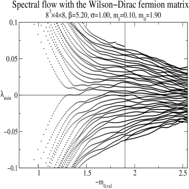
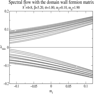
In our unquenched test runs such a gap does not appear (see figure 2). The lattice spacing is obviously still too large. The spectrum flow of $D_{F}$ on the smae gauge configuration is shown by figure 3.

Figure 3: Eigenvalue flow for the hermitean domain wall fermion matrix.

The conclusion of our first tests is that the application of the TSMB algorithm for numerical simulations of domain wall quarks is straightforward. A comparison of the computation speed compared to, say, Wilson quarks requires an analysis including the measurement of autocorrelations. Since the good chiral properties of domain wall fermions develop only sufficiently close to the continuum limit, the performance studies have to be carried out on large lattices.

References

- [1] D.B. Kaplan, Phys. Lett. B288 (1992) 342.
- [2] R. Narayanan, H. Neuberger, Phys. Lett. B302 (1993) 62.
- [3] Y. Shamir, Nucl.Phys. B406 (1993) 90.
- [4] I. Montvay, Nucl. Phys. B466 (1996) 259.
- [5] I. Montvay, Comput. Phys. Commun. 109 (1998) 144.
- [6] I. Montvay, in “Numerical challenges in lattice quantum chromodynamics”, Wuppertal 1999, Springer 2000, p. 153; hep-lat/9911014.
- [7] I. Montvay, Int. J. Mod. Phys. A17 (2002) 2377.
- [8] qq+q Collaboration, F. Farchioni et al., to appear in Eur. Phys. J. C; hep-lat/0206008.
- [9] qq+q Collaboration, F. Farchioni et al., these proceedings.
- [10] I. Montvay, Phys. Lett. B537 (2002) 69.
- [11] P.M. Vranas, Phys. Rev. D57 (1998) 1415.
- [12] M. Lüscher, Nucl. Phys. B418 (1994) 637.
- [13] P. Chen et al., Phys. Rev. D64 (2001) 014503.
- [14] CP-PACS Collaboration, A. Ali Khan et al., Phys. Rev. D63 (2001) 114504.