Strange matrix elements of the nucleon

Abstract

Results for the disconnected contributions to matrix elements of the vector current and scalar density have been obtained for the nucleon from the Wilson action at $\beta=6$ using a stochastic estimator technique and 2000 quenched configurations. Various methods for analysis are employed and chiral extrapolations are discussed.

1 MOTIVATION

Prediction, measurement and understanding of strangeness in the nucleon have proven to be significant challenges for both theory and experiment. Of particular interest at present are the strangeness electric and magnetic form factors. Experimental results have been reported by SAMPLE[1] and HAPPEX[2], and other groups are also planning experiments.[3]

A number of lattice QCD studies have been reported during the past few years[4, 5], though the conclusions are somewhat varied. In the present work we report the results of a high statistics simulation. Different analysis techniques are studied and chiral extrapolations are discussed. The strangeness scalar density and electric and magnetic form factors are all analyzed together, and results are compared to experimental data.

2 SIMULATIONS AND ANALYSIS

The nucleon’s strangeness form factors arise from a disconnected strange quark loop that we compute stochastically using real $Z_{2}$ noise[6]. To reduce the variance, the first four terms of the perturbative quark matrix are subtracted.[7] (For the scalar density, the first five terms are subtracted.) The three matrix elements of interest are

$$M_{\{S,M,E\}}(t,\vec{q})=\left\{G_{S}^{(s)},\frac{q_{j}G_{M}^{(s)}}{E_{q}+m},G_{E}^{(s)}\right\}$$ (1)

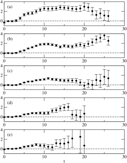
where $\left<N\left|\bar{s}s\right|N\right>=Z_{S}G_{S}^{(s)}$, $Z_{S}\approx 1-3\kappa_{v}/(4\kappa_{c})$, and the $M_{X}(t,\vec{q})$ can be extracted from the ratios

$$R_{X}(t,t^{\prime},\vec{q})=\frac{G_{X}^{(3)}(t,t^{\prime},\vec{q})G^{(2)}(t^{\prime},\vec{0})}{G^{(2)}(t,\vec{0})G^{(2)}(t^{\prime},\vec{q})}$$ (2)

of 2 and 3-point correlators by various methods:

$$\sum_{t^{\prime}=1}^{t+1}\left[R_{X}(t,t^{\prime},\vec{q})-R_{X}(t\!-\!1,t^{\prime},\vec{q})\right]\to M_{X}(t,\vec{q}),$$ (3)

$$\sum_{t^{\prime}=1}^{t}R_{X}(t,t^{\prime},\vec{q})\to{\rm constant}+tM_{X}(t,\vec{q}),$$ (4)

$$\sum_{t^{\prime}=1}^{t_{fixed}}R_{X}(t,t^{\prime},\vec{q})\to{\rm constant}+tM_{X}(t,\vec{q}).$$ (5)

Any authentic signal should be visible with each of these methods, and should be consistent among all of them.[5]

Figure 1: $M_{S}(t,\vec{q})$ from Eq. (3) with $\kappa_{v}=\kappa_{l}=0.152$. From top to bottom, the plots show $\vec{q}_{L}^{\,2}=0$, 1, 2, 3 and 4, where $\vec{q}_{L}\equiv(10a/\pi)\vec{q}$.

Simulations have been performed on $20^{3}\times 32$ lattices using the Wilson action with $\beta=6$. Dirichlet time boundaries are used for quarks with the source five timesteps from the lattice boundary. Valence quarks use $\kappa_{v}=0.152$, 0.153 and 0.154. The chiral limit is $\kappa_{c}\approx 0.1571$ and our $\kappa_{v}$ values are in the strange region. The mass of the quark in the loop will be held fixed at a value corresponding to $\kappa_{l}=0.152$ and the analysis will be based on 2000 configurations with 60 $Z_{2}$ noises per configuration. Consistent results (not shown in this brief article) have been obtained from the analysis of 100 configurations with $\kappa_{l}=0.154$ and 200 $Z_{2}$ noises per configuration.

Results for $M_{S}(t,\vec{q})$ from Eq. (3) are shown in Fig. 1. For each $\vec{q}$ considered, a clear plateau begins about 10 timesteps from the source. (The source is at $t=0$ in the plots.) On the other hand, results for $M_{M}(t,\vec{q})$ and $M_{E}(t,\vec{q})$ are consistent with zero for each $\vec{q}$ and $\kappa_{v}$ as shown in Table 1.

3 CHIRAL FITS

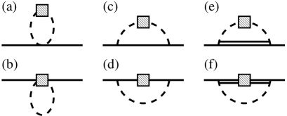
Quark mass and momentum dependences can be calculated analytically within quenched chiral perturbation theory from the diagrams of Fig. 2 as well as all tree-level counterterms.

Table 1: Fits to the matrix elements of Eq. (3) beginning 10 timesteps from the source. $\vec{q}_{L}\equiv(10a/\pi)\vec{q}$.

$\kappa_{v}$	$\vec{q}_{L}^{\,2}$	$\kappa_{l}=0.152$
		$G_{S}^{(s)}$		$G_{M}^{(s)}$		$G_{E}^{(s)}$
0.152	0	2.	6(4)	—		-0.	009(13)
	1	1.	7(2)	0.	007(16)	-0.	008(8)
	2	1.	2(2)	-0.	018(14)	0.	012(10)
	3	1.	1(5)	-0.	014(23)	0.	008(17)
	4	0.	7(6)	0.	004(31)	0.	026(40)
0.153	0	2.	7(5)	—		-0.	010(15)
	1	1.	8(3)	0.	012(22)	-0.	011(10)
	2	1.	3(2)	-0.	021(20)	0.	015(14)
	3	1.	2(6)	-0.	018(32)	0.	008(22)
	4	0.	7(8)	0.	005(48)	0.	029(56)
0.154	0	2.	9(5)	—		-0.	013(19)
	1	1.	8(3)	0.	019(33)	-0.	014(15)
	2	1.	3(3)	-0.	022(31)	0.	019(21)
	3	1.	5(9)	-0.	029(53)	0.	008(32)
	4	0.	8(11)	0.	010(82)	0.	021(81)

There are six independent parameters and we consider two extreme limits: either the quenched $\eta^{\prime}$ is absent ($\gamma=0$), or $\gamma\neq 0$ but the non-$\eta^{\prime}$ parameters are set to zero in the loops. The physical situation must lie between these two extremes, and so we expect the true values to be somewhere between the curves in Fig. 3. (For another recent discussion of chiral fitting, see Ref. [8].)

Figure 2: Leading loop diagrams from quenched chiral perturbation theory. Dashed, solid and double lines denote octet mesons, octet baryons and decuplet baryons respectively. A shaded box denotes a current insertion.

Figure 3: Lattice results extrapolated to the physical hadron masses.

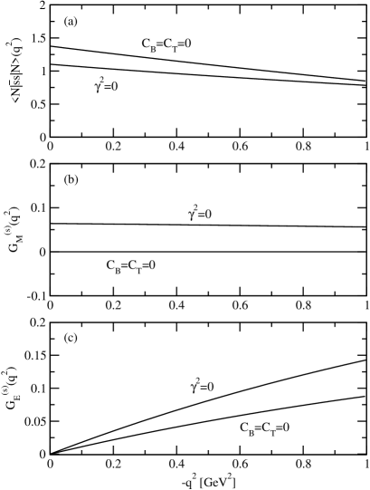
4 COMPARING TO EXPERIMENT

The results of Figure 3 compare to the existing experimental results as follows:

$$G_{M}^{(s)}(q_{1}^{2})=\left\{\begin{array}[]{ll}0.14\pm 0.29\pm 0.31,&{\rm~{}Ref.~{}\cite[cite]{[\@@bibref{}{SAMPLE}{}{}]}}\\ 0.03\pm 0.03,&{\rm~{}Fig.~{}\ref{figfinal}}\end{array}\right.$$ (6)

$$G_{E}^{(s)}(q_{2}^{2})+0.39G_{M}^{(s)}(q_{2}^{2})$$ (9)

$$=\left\{\begin{array}[]{ll}0.025\pm 0.020\pm 0.014,&{\rm~{}Ref.~{}\cite[cite]{[\@@bibref{}{HAPPEX}{}{}]}}\\ 0.027\pm 0.016,&{\rm~{}Fig.~{}\ref{figfinal}}\end{array}\right.$$

where $-q_{1}^{2}=0.1$ GeV² and $-q_{2}^{2}=0.477$ GeV². For the scalar density, we find

$$(m_{s}/m_{N})\left<N\left|\bar{s}s\right|N\right>(0)=0.15(2),$$ (10)

which can be compared to the result of 0.195(9) reported in Ref. [9].

We have not attempted to estimate the sizes of systematic uncertainties in our results due, for example, to quenching and to the use of chiral extrapolations for valence quarks in the strange region. The raw lattice data of Table 1 show, at best, only tiny strange quark effects over the range of momenta and quark masses that were studied. Large strange-quark loop contributions in the vector current matrix elements should be considered unlikely.

References

- [1] R. Hasty et. al., Science 290, 2117 (2000).
- [2] K.A. Aniol et. al., Phys. Lett. B509, 211 (2001).
- [3] For example, the A4 Collaboration at MAMI and the G0 Collaboration at Jefferson Lab.
- [4] S.J. Dong, K.F. Liu and A.G. Williams, Phys. Rev. D58, 074504 (1998); D.B. Leinweber and A.W. Thomas, Phys. Rev. D62, 07505 (2000); N. Mathur and S.J. Dong, Nucl. Phys. (P.S.) 94, 311 (2001); W. Wilcox, Nucl. Phys. (P.S.) 94, 319 (2001).
- [5] R. Lewis, W. Wilcox and R.M. Woloshyn, hep-ph/0201190 (2002).
- [6] S.J. Dong and K.F. Liu, Nucl. Phys. (P.S.) 26, 353 (1992); Phys. Lett. B328, 130 (1994).
- [7] C. Thron, S.J. Dong, K.F. Liu and H.P. Ying, Phys. Rev. D57, 1642 (1998); W. Wilcox, hep-lat/9911013, in Numerical Challenges in Lattice Quantum Chromodynamics, edited by A. Frommer et. al. (Springer Verlag, Heidelberg, 2000); Nucl. Phys. (P.S.) 83, 834 (2000); C. Micheal, M.S. Foster and C. McNeile, Nucl. Phys. (P.S.) 83, 185 (2000).
- [8] J.W. Chen and M.J. Savage, hep-lat/0207022.
- [9] S.J. Dong, J.F. Lagaë and K.F. Liu, Phys. Rev. D54, 5496 (1996).