An Exact Algorithm for Any-flavor Lattice QCD with Kogut-Susskind Fermion

Abstract

We propose an exact simulation algorithm for lattice QCD with dynamical Kogut-Susskind fermion in which the $N_{f}$-flavor fermion operator is defined as the $N_{f}/4$-th root of the Kogut-Susskind (KS) fermion operator. The algorithm is an extension of the Polynomial Hybrid Monte Carlo (PHMC) algorithm to KS fermions. The fractional power of the KS fermion operator is approximated with a Hermitian Chebyshev polynomial, with which we can construct an algorithm for any number of flavors. The error which arises from the approximation is corrected by the Kennedy-Kuti noisy Metropolis test. Numerical simulations are performed for the two-flavor case for several lattice parameters in order to confirm the validity and the practical feasibility of the algorithm. In particular tests on a $16^{4}$ lattice with a quark mass corresponding to $m_{\mathrm{PS}}/m_{\mathrm{V}}\sim 0.68$ are successfully accomplished. We conclude that our algorithm provides an attractive exact method for dynamical QCD simulations with KS fermions.

, , , , , , , , , , , , , and

1 Introduction

In numerical studies of lattice QCD, advancing simulations including dynamical quarks is the most pressing issue to confirm the validity of QCD and to extract low energy hadronic properties from it. While including dynamical quark effects is still a difficult task, recent developments of computational power and algorithms have enabled dynamical simulations of reasonable scale. Much efforts are thus being spent to accurately compute physical quantities in full QCD simulations [1, 2, 3, 4, 5, 6, 7].

A large number of these simulations are being made with Wilson-type fermion action using the Hybrid Monte Carlo (HMC) algorithm [8, 9], which is one of the exact dynamical fermion algorithms. A limitation of the HMC algorithm is that the number of flavors has to be even to express the fermion determinant in terms of pseudo-fermion fields. Recently, however, the polynomial Hybrid Monte Carlo (PHMC) algorithm [10, 11] has been proposed to simulate the odd number of flavors with Wilson-type fermion as an exact algorithm [12, 13]. The combination of the HMC and PHMC algorithms enables us to simulate the realistic world of 2+1-flavors of quarks with lattice QCD [12, 13].

The Kogut-Susskind (KS) fermion action has also been widely used in full QCD simulations. For the KS action, the application of the HMC algorithm is restricted to a multiple of four flavors due to the four-fold Dirac fermion content of a single KS fermion. Even if one adopts the usual assumption that the $1/4$ power of the KS fermion determinant provides a lattice discretization of a single Dirac fermion determinant, efficient exact algorithms have not been known for two- or single-flavor quark with the KS formalism. For this reason, dynamical KS fermion simulations for two- or three-flavor QCD are made with the $R$-algorithm [14] even today, which is an approximate algorithm.

The $R$-algorithm involves a systematic error from a finite step size of the molecular dynamics integrator. Strictly speaking, a careful extrapolation of physical quantities to the zero step size is required. Since this is too computer time consuming, numerical simulations are usually carried out at a finite step size which is chosen so that the systematic error is considered invisible compared to the statistical error. While checks on small lattices are usually made to ensure smallness of the systematic error at least for several quantities, the possibility that other physical quantities are spoiled by the finite step size effects is difficult to exclude. Even such checks become progressively more difficult as smaller quark masses require vastly increasingly computer time. Clearly, an exact and efficient algorithm is desired for dynamical QCD simulations with the KS fermion action not only for two flavors but also for a single flavor of quarks.

In this article, we propose an exact algorithm for KS fermions which is capable of simulating an arbitrary number of flavors. Our algorithm is an application of the PHMC algorithm. It is an extension of the idea of the Rational Hybrid Monte Carlo (RHMC) algorithm [15] put forward by Horváth, Kennedy, and Sint a few years ago. They briefly described their idea and tested their algorithm together with the PHMC algorithm for two- and four-flavor QCD with the KS fermions on a small size lattices. We shall comment on the difference between their algorithm and ours below. Recently Hasenfratz and Knechtli [16] also proposed an exact algorithm for KS fermions with hyper-cubic smeared links, which makes use of the polynomial approximation and global update algorithm. The algorithm is considered to be effective for the action for which the HMC type algorithm cannot be applied.

The outline of our algorithms goes as follows. Applying a polynomial approximation to the fractional power of the KS fermion matrix, we rewrite the original partition function to a form suitable for the PHMC algorithm. The resulting effective partition function has two parts; one part is described by an effective action for the polynomial approximation of the fermion action, which can be treated by the HMC algorithm. The other part is the correction term which removes the systematic errors from the polynomial approximation. The correction term can be evaluated by the Kennedy-Kuti [17] noisy Metropolis test, which has been successfully used in the multi-boson algorithm [18]. With this combination, we can make an exact algorithm for KS fermions. In this work we describe the details of the algorithm, and report results of our numerical test on the applicability of the algorithm to realistic simulations.

Since the polynomial approximation to rewrite the partition function is not unique, there can be several realizations of the PHMC algorithm for the KS fermion. We construct two types of realizations of the polynomial approximation to the PHMC algorithm with $N_{f}$ quark flavors:

Case A

Use a polynomial which approximates the $N_{f}/8$ power of the KS fermion matrix which corresponds to $N_{f}/2$ quark flavors. Introducing a single pseudo-fermion field with squaring the fermion matrix, we obtain $N_{f}$ flavors of quarks.

Case B

Use an even-order polynomial which approximates the $N_{f}/4$ power of the KS fermion matrix, which corresponds to $N_{f}$ flavors of quarks. To express $N_{f}$ quark flavor with a single pseudo-fermion field, the even-order polynomial is factored into a product of two polynomials using the method by Alexandrou et al. [19].

We estimate the computational cost of the two algorithms in terms of the number of multiplication by the KS fermion matrix, and find that the algorithm B is roughly a factor two more efficient.

We investigate the property and efficiency of the Chebyshev polynomial approximation as an example of the polynomial approximation. The method to split the even-order polynomial into two polynomials, which is used in case B, is also described. The limitation of our method for splitting the even-order polynomial is discussed.

The Kennedy-Kuti noisy Metropolis test involves a non-trivial factor. Since we take the fractional power of the KS operator, the correction term also includes fractional powers of fermion matrices. In order to evaluate the measure for the noisy Metropolis test acceptance rate, we need to evaluate the fractional power of the correction matrix. To do this, we make use of the Lanczos-based Krylov subspace method by Boriçi [20], originally proposed for the inverses square root of the squared Hermitian Wilson-Dirac operator in the Neuberger’s overlap fermion. We modify the Boriçi’s algorithm to our purpose.

Finally we investigate the validity and property of the PHMC algorithm (case B) in the case of two flavors of quarks numerically. We first confirm that our algorithm works correctly using a small lattice of a size $8^{3}\times 4$, where a comparison to the $R$-algorithm is performed. On an $8^{3}\times 16$ lattice we investigate the mass dependence of the algorithm. We find that for quark masses lighter than $m_{\mathrm{PS}}/m_{\mathrm{V}}\sim 0.60$ the polynomial with order larger than $O(600)$ is required. Finally, we apply our algorithm to a moderately large lattice of $16^{4}$ with a rather heavy quark mass $m_{\mathrm{PS}}/m_{\mathrm{V}}\sim 0.69$ as a prototype for future realistic simulations. On this lattice violation of reversibility and convergence of the Lanczos-based Krylov subspace method for the noisy Metropolis test are investigated. We find satisfactory results; there is no visible reversibility violation, and the Krylov subspace method converges within the limit of double precision arithmetic. The test run on the large size lattice shows reasonable efficiency on the computational time.

The rest of the paper is organized as follows. In section 2, we introduce the lattice QCD partition function with the KS fermions, and rewrite it to a form suitable for the PHMC algorithm. We give two forms for the partition function as described above. The outline of the PHMC algorithm is also shown in this section. In section 3, we describe the Chebyshev polynomial as a specific choice for the polynomial approximation. The error of the polynomial approximation is investigated. The molecular dynamics (MD) step with the polynomial approximation in the PHMC algorithm is explained in section 4. The details of the noisy Metropolis test is given in section 5. We estimate the computational cost of the algorithms in section 6, where we find that the case B algorithm is better. In section 7, we show the test results with the PHMC algorithm. Conclusions are given in the last section.

2 Effective Action for PHMC algorithm

The QCD partition function for $N_{f}$ flavors of quarks using the KS fermion is defined by

$$Z=\int{\mathcal{D}}U\det[D]^{N_{f}/4}e^{-S_{g}[U]},$$ (2.1)

where $S_{g}[U]$ is the gauge action, $U_{\mu}(n)$ is gauge links, and $\det[D]$ is the determinant of the KS fermion operator $D$. The KS fermion operator $D$ is defined by

$$D(n,m)=am\delta_{n,m}+\frac{1}{2}\sum_{\mu}\eta_{\mu}(n)\left[U_{\mu}(n)\delta_{n+\hat{\mu},m}-U^{{\dagger}}_{\mu}(n-\hat{\mu})\delta_{n-\hat{\mu},m},\right].$$ (2.2)

where $am$ is the bare quark mass with lattice unit $a$, and $\eta_{\mu}(n)$ is the usual KS fermion phase. In our work we adopt the usual assumption that taking the fourth root of the KS fermion operator represents a lattice discretization of a single Dirac fermion operator in the continuum.

The determinant of the KS fermion operator can be rewritten as

$$\det[D]=\det\left[\begin{array}[]{cc}am\mathbf{1}_{ee}&M_{eo}\\ M_{oe}&am\mathbf{1}_{oo}\end{array}\right]=\det\left[\begin{array}[]{cc}\mathbf{1}_{ee}&0\\ 0&\hat{D}_{oo}\end{array}\right],$$ (2.3)

where $\hat{D}_{oo}=(am)^{2}\mathbf{1}_{oo}-M_{oe}M_{eo}$ with $M_{eo}(M_{oe})$ the hopping matrix from odd site to even site (even site to odd site) defined in Eq. (2.2). Since $\hat{D}_{oo}$ is nothing but the odd part of $D^{{\dagger}}D$, the eigenvalues are real and positive semi-definite, which enable us to take the fractional power of the KS fermion operator except for vanishing quark masses. Thus the QCD partition function is reduced to

$$Z=\int{\mathcal{D}}U\det[\hat{D}_{oo}]^{N_{f}/4}e^{-S_{g}[U]}.$$ (2.4)

To apply the PHMC algorithm, we approximate the fractional power of $\hat{D}_{oo}$ by a polynomial of $\hat{D}_{oo}$. We consider two methods for the polynomial approximation. We restrict ourselves to the case that the number of flavors is one or two. Generalization to any integer flavors is achieved by combining the single-flavor and two-flavor cases.

Case A

We introduce a polynomial $P_{N_{\mathrm{poly}}}[x]$ of order $N_{\mathrm{poly}}$, which approximates $x^{-N_{f}/8}$ for real and positive (non-zero) $x$ as

$$x^{-N_{f}/8}\sim P_{N_{\mathrm{poly}}}[x]=\sum_{i=0}^{N_{\mathrm{poly}}}c_{i}x^{i},$$ (2.5)

where $c_{i}$’s are real coefficients. The property that the eigenvalues of the KS fermion operator $\hat{D}_{oo}$ are bounded below by $(am)^{2}$ enables us to substitute $\hat{D}_{oo}$ into Eq. (2.5) to approximate the fractional power of the KS fermion operator. Using this polynomial, we can rewrite the determinant as

$$\det\left[\hat{D}_{oo}\right]^{N_{f}/4} = \left(\frac{\det\left[\hat{D}_{oo}\left(P_{N_{\mathrm{poly}}}[\hat{D}_{oo}]\right)^{8/N_{f}}\right]}{\det\left[\left(P_{N_{\mathrm{poly}}}[\hat{D}_{oo}]\right)^{8/N_{f}}\right]}\right)^{N_{f}/4}$$ (2.6)

$$= \frac{\det\left[W[\hat{D}_{oo}]\right]^{N_{f}/4}}{\det\left[P_{N_{\mathrm{poly}}}[\hat{D}_{oo}]\right]^{2}},$$

where we introduced

$$W[\hat{D}_{oo}]=\hat{D}_{oo}\left(P_{N_{\mathrm{poly}}}[\hat{D}_{oo}]\right)^{8/N_{f}},$$ (2.7)

whose deviation from the identity matrix indicates the residual of the polynomial approximation. We refer to $W[\hat{D}_{oo}]$ as the correction matrix. Note that the exponent of $P_{N_{\mathrm{poly}}}$ becomes an integer when $N_{f}=2$ or $N_{f}=1$ as we assumed. Introducing pseudo-fermion fields to the denominator of Eq. (2.6), we obtain

$$\det\left[\hat{D}_{oo}\right]^{N_{f}/4} = \det\left[W[\hat{D}_{oo}]\right]^{N_{f}/4}\int{\mathcal{D}}\phi_{o}^{{\dagger}}{\mathcal{D}}\phi_{o}e^{-S_{q}[U,\phi_{o}^{{\dagger}},\phi_{o}]},$$ (2.8)

$$S_{q}[U,\phi_{o}^{{\dagger}},\phi_{o}] = \left|P_{N_{\mathrm{poly}}}[\hat{D}_{oo}]\phi_{o}\right|^{2}.$$ (2.9)

Thus the QCD partition function Eq. (2.4) becomes

$$Z=\int{\mathcal{D}}U{\mathcal{D}}\phi_{o}^{{\dagger}}{\mathcal{D}}\phi_{o}\det[W[\hat{D}_{oo}]]^{N_{f}/4}e^{-S_{g}[U]-S_{q}[U,\phi_{o}^{{\dagger}},\phi_{o}]}.$$ (2.10)

Case B

We define a polynomial $P_{N_{\mathrm{poly}}}[x]$ with $N_{\mathrm{poly}}$ even to approximate $x^{-N_{f}/4}$ for real and positive (non-zero) $x$ by

$$x^{-N_{f}/4}\sim P_{N_{\mathrm{poly}}}[x]=\sum_{i=0}^{N_{\mathrm{poly}}}c_{i}x^{i}.$$ (2.11)

Similarly to the case A, we can rewrite the determinant as

$$\det\left[\hat{D}_{oo}\right]^{N_{f}/4} = \left(\frac{\det\left[\hat{D}_{oo}\left(P_{N_{\mathrm{poly}}}[\hat{D}_{oo}]\right)^{4/N_{f}}\right]}{\det\left[\left(P_{N_{\mathrm{poly}}}[\hat{D}_{oo}]\right)^{4/N_{f}}\right]}\right)^{N_{f}/4}$$ (2.12)

$$= \frac{\det\left[W[\hat{D}_{oo}]\right]^{N_{f}/4}}{\det\left[P_{N_{\mathrm{poly}}}[\hat{D}_{oo}]\right]},$$

where

$$W[\hat{D}_{oo}]=\hat{D}_{oo}\left(P_{N_{\mathrm{poly}}}[\hat{D}_{oo}]\right)^{4/N_{f}}.$$ (2.13)

For $N_{\mathrm{poly}}$ even, $P_{N_{\mathrm{poly}}}[x]$ can be factored into two polynomials as employed in the multi-boson algorithm for single-flavor QCD [19]. Making use of this property, we obtain

$$\det\left[\hat{D}_{oo}\right]^{\frac{N_{f}}{4}}=\frac{\det\left[W[\hat{D}_{oo}]\right]^{N_{f}/4}}{\left|\det\left[Q_{N_{\mathrm{poly}}}[\hat{D}_{oo}]\right]\right|^{2}},$$ (2.14)

where $Q_{N_{\mathrm{poly}}}[x]$ is defined by

$$\left|Q_{N_{\mathrm{poly}}}[x]\right|^{2}=P_{N_{\mathrm{poly}}}[x],\ \ \ \ Q_{N_{\mathrm{poly}}}[x]=\sum^{N_{\mathrm{poly}}/2}_{i=0}d_{i}x^{i},$$ (2.15)

with complex coefficients $d_{i}$. The factoring is not unique. In the next section we describe the method for dividing the polynomial. Introducing pseudo-fermion fields to the denominator of Eq. (2.14), we obtain the QCD partition function for the PHMC algorithm in the case B as

$$Z = \int{\mathcal{D}}U{\mathcal{D}}\phi_{o}^{{\dagger}}{\mathcal{D}}\phi_{o}\det[W[\hat{D}_{oo}]]^{N_{f}/4}e^{-S_{g}[U]-S_{q}[U,\phi_{o}^{{\dagger}},\phi_{o}]},$$ (2.16)

$$S_{q}[U,\phi_{o}^{{\dagger}},\phi_{o}] = \left|Q_{N_{\mathrm{poly}}}[\hat{D}_{oo}]\phi_{o}\right|^{2}.$$ (2.17)

The PHMC algorithm follows two steps:

1. The HMC step with the effective action Eq. (2.10) for the case A (Eq. (2.16) for the case B).

2. The noisy Metropolis test to remove the systematic error represented by $W[\hat{D}_{oo}]$ in Eq. (2.6) for the case A (Eq. (2.14) for the case B).

The noisy Metropolis test in step (2) has been used in the multi-boson algorithm [18]. The reweighting technique [11] and stochastic noisy estimator [12] method can be applied to remove the systematic error. In this paper we employ the noisy Metropolis test to make our algorithm exact [18, 6].

The original idea by Horváth et al. differs from ours. We separate the action into two pieces; the effective action with polynomial approximation and the correction factor. They do not separate the full action and apply the Kennedy-Kuti noisy estimator for the energy conservation violation $dH$ itself to make the algorithm exact, while we apply the method to the correction factor. It is not known which approach is more efficient. We leave a study of this issue to future work as a comparison of the two algorithms is beyond the scope of the present paper.

3 Polynomial approximation

We employ the Chebyshev polynomial approximation to $x^{-s}$ with a real positive $x$, where $s$ takes the following values: $1/2$, $1/4$, $1/8$, depending on the choice of case A or B, and on $N_{f}$. We explain the application to the KS fermion operator and investigate the relation among the order of polynomial, the residual of the approximation, and the choice of case A or B.

Several polynomial approximations for $1/x$ have been proposed in studies of the multi-boson algorithm. They include Chebyshev [21], adapted [22], and least square [23] polynomials. The choice of the polynomial affects the efficiency, i.e., how much one can decrease the polynomial order so as to make the correction matrix as close to the unit matrix as possible. Since this is not a problem of the simulation algorithm itself, we employ the simple choice of the Chebyshev polynomial approximation for the fractional power of the KS fermion operator.

3.1 Chebyshev approximation

The Chebyshev polynomial expansion of $x^{-s}$ is

$$x^{-s}=\left[1+(1-\epsilon)y\right]^{-s}=\sum_{k=0}^{\infty}c_{k}T_{k}[y],$$ (3.1)

where $y=(x-1)/(1-\epsilon)$, $\epsilon$ is optimized so as to satisfy $y\in[-1,1]$ depending on the support of $x$ and $\epsilon\in(0,1)$. We restrict the support of exponent $s$ to $s\in(0,1]$.   $T_{k}[x]$ is the $k$-th order Chebyshev polynomial defined by

$$T_{k}[x]=\cos(k\arccos(x)).$$ (3.2)

The polynomial has the following recurrence formula:

$$T_{k}[x]=\alpha_{k-1}xT_{k-1}[x]+\beta_{k-2}T_{k-2}[x]\ \ \ (k\geq 1),$$ (3.3)

where $\alpha_{k}=2/(1+\delta_{k,0})$ ($k\geq 0$), $\beta_{-1}=0$, $\beta_{k}=-1$ ($k\geq 0$), and $T_{0}[x]=1$. The Chebyshev polynomial expansion coefficients $c_{k}$ in Eq. (3.1) are calculated as

$$c_{k} = {\int_{-1}}^{1}[1+(1-\epsilon)y]^{-s}\frac{T_{k}[y]}{\sqrt{1-y^{2}}}dy$$ (3.4)

$$= \frac{2r^{k}}{1+\delta_{k,0}}(1+r^{2})^{s}F(s,s+k;1+k;r^{2})\frac{\Gamma(s+k)}{\Gamma(s)\Gamma(1+k)},$$

where $r=\left(-1+\sqrt{\epsilon(2-\epsilon)}\right)/(1-\epsilon)$, $F(\alpha,\beta;\gamma;z)$ Gaussian hyper-geometric function, and $\Gamma(z)$ Gamma function. Truncating Eq. (3.1) at order $N_{\mathrm{poly}}$, we approximate $x^{-s}$ by

$$x^{-s}=\left[1+(1-\epsilon)y\right]^{-s}\sim P_{N_{\mathrm{poly}}}[x]=\sum_{k=0}^{N_{\mathrm{poly}}}c_{k}T_{k}[y].$$ (3.5)

The truncation error is bounded by

$$\left|x^{-s}-P_{N_{\mathrm{poly}}}[x]\right|\leq\frac{2}{\Gamma(s)}\left(\frac{1+r^{2}}{1-r^{2}}\right)^{s}\frac{(-r)^{N_{\mathrm{poly}}+1}}{1+r},$$ (3.6)

where $r$ takes a value in the region $-1\leq r\leq 0$. This inequality is not optimal. It demonstrates, however, an exponential decrease of the residual with increasing $N_{\mathrm{poly}}$. When $\epsilon\ll 1$, it is expected that $N_{\mathrm{poly}}\propto\sqrt{\epsilon}$ at a constant residual.

The operator corresponding to $y$ in the above relation is given by shifting and changing the normalization of the KS fermion operator:

$$\hat{D^{\prime}}_{oo}=\mathbf{1}_{oo}-(a\lambda)^{2}\hat{M}_{oo}=\frac{2}{2(am)^{2}+(a\Lambda_{\mathrm{max}})^{2}}\hat{D}_{oo},$$ (3.7)

where $(a\lambda)^{2}=2(a\Lambda_{\mathrm{max}})^{2}/(4(am)^{2}+2(a\Lambda_{\mathrm{max}})^{2})$, and $\hat{M}_{oo}=\mathbf{1}_{oo}+2M_{oe}M_{eo}/(a\Lambda_{\mathrm{max}})^{2}$. $a\Lambda_{\mathrm{max}}$ is introduced to keep all eigenvalues of $-\hat{M}_{oo}$ in the domain $[-1,1]$. Since the normalization in front of $\hat{D}_{oo}$ in Eq. (3.7) can be absorbed into the normalization of the partition function, we use $\hat{D^{\prime}}_{oo}$ instead of $\hat{D}_{oo}$ and omit the prime symbol from $\hat{D^{\prime}}_{oo}$ in the rest of the paper. For the free case, $a\Lambda_{\mathrm{max}}=2$ is sufficient to satisfy the condition for the eigenvalues of $-\hat{M}_{oo}$. In the interacting case, it becomes larger than two. This is seen, for example, in a study for SU(2) lattice gauge theory where the complete eigenvalue distribution has been investigated [25]. With this expression for the KS fermion operator, the polynomial approximation of $\hat{D}_{oo}^{-s}$ becomes

$$\hat{D}_{oo}^{-s}\sim P_{N_{\mathrm{poly}}}[\hat{D}_{oo}]=\sum_{i=0}^{N_{\mathrm{poly}}}c_{k}T_{k}[-\hat{M}_{oo}],$$ (3.8)

where $c_{i}$ is obtained from Eq. (3.4) with $\epsilon=1-(a\lambda)^{2}$. The exponent $s$ is chosen to be $s=N_{f}/8$ for the case A and $s=N_{f}/4$ for the case B.

For the case B, we have to solve Eq. (2.15) to obtain the half-order polynomial $Q_{N_{\mathrm{poly}}}$. Here we choose to construct $Q_{N_{\mathrm{poly}}}$ so as to have the form of the Chebyshev polynomial expansion as Eq. (3.8). Since this problem is rather complicated, we postpone the discussion to the subsection at the end of this section, and proceed assuming that the polynomial $Q_{N_{\mathrm{poly}}}$ and its coefficients $d_{i}$ are already given.

Given the Chebyshev polynomial expansion coefficients $c_{m}$ ($d_{m}$), we can evaluate the polynomial $P_{N_{\mathrm{poly}}}[x]$ ($Q_{N_{\mathrm{poly}}}[x]$) using the Clenshaw’s recurrence formula (for example, see [26]). When $x$ is the KS fermion operator $\hat{D}_{oo}$, the multiplication of the operator $P_{N_{\mathrm{poly}}}[\hat{D}_{oo}]$ on a vector $v_{o}$ is carried out by the following three step recurrence formula:

$$y^{(k)}_{o}=\alpha_{k}(-\hat{M}_{oo})y^{(k+1)}_{o}+\beta_{k}y^{(k+2)}_{o}+c_{k}v_{o},$$ (3.9)

where $y^{(k)}$ is a working vector labeled $k$, $\alpha_{k}$ and $\beta_{k}$ are given in Eq. (3.3), and $c_{k}$ is the Chebyshev polynomial expansion coefficient. Solving for $y^{(k)}_{o}$ with this equation from $k=N_{\mathrm{poly}}$ to $k=0$ with the initial condition $y^{(N_{\mathrm{poly}})}_{o}=y^{(N_{\mathrm{poly}}+1)}_{o}=0$, we obtain

$$P_{N_{\mathrm{poly}}}[\hat{D}_{oo}]v_{o}=y^{(0)}_{o}.$$ (3.10)

For $Q_{N_{\mathrm{poly}}}[\hat{D}_{oo}]v_{o}$, $d_{k}$ is used instead of $c_{k}$ and $k$ runs from $N_{\mathrm{poly}}/2$ to $0$. Note that we need not store all working vectors $y^{(k)}_{o}$; only two working vectors are required for the computation. This method can be applied to any matrix polynomial which has the same structure for the recurrence relation as Eq. (3.3). The computational cost to calculate $P_{N_{\mathrm{poly}}}[\hat{D}_{oo}]v_{o}$ ($Q_{N_{\mathrm{poly}}}[\hat{D}_{oo}]v_{o}$) is $N_{\mathrm{poly}}$ ($N_{\mathrm{poly}}/2$) by means of the number of matrix-vector multiplication.

Figure 1: $R(x)$ as a function of $y=(x-1)/(1-\epsilon)$ at $N_{\mathrm{poly}}/s=800,\epsilon=1/1000$.

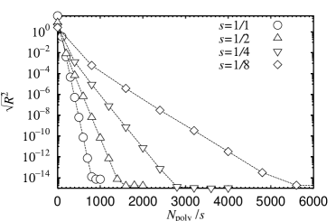
Figure 2: $N_{\mathrm{poly}}/s$ dependence of the integrated residuals $\sqrt{R^{2}}$. $\epsilon=1/1000$ are plotted.

Now we discuss the quality of the polynomial approximation. We evaluate the polynomial approximation residual using

$$R(x)=\left|x(P_{N_{\mathrm{poly}}}[x])^{1/s}-1\right|.$$ (3.11)

Figure 1 shows the residual of the approximation as a function of $y=(x-1)/(1-\epsilon)$. The calculation is performed using Clenshaw’s recurrence in double precision arithmetic. In order to compare the approximation at the fixed computational cost, the number of matrix-vector multiplication, in calculating the correction matrix irrespective of the choice of $s$ (case A or B and $N_{f}$), we keep $N_{\mathrm{poly}}/s$ constant ($N_{\mathrm{poly}}/s=800$) as an example. We observe that the approximation becomes worse for smaller $s$ ($s=1$ case reaches the limit of double precision arithmetic). We also investigate the $N_{\mathrm{poly}}/s$ dependence of the polynomial approximation. In figure 2 we plot the $N_{\mathrm{poly}}/s$ dependence of the residual defined by

$$\sqrt{R^{2}}=\sqrt{{\int_{-1}}^{1}dyR(x(y))^{2}}.$$ (3.12)

Clear exponential decay is observed. The dependence of the slope on the choice of $s$ indicates that the computational cost increases with decreasing $s$. In our case, defining the polynomial order by $N_{\mathrm{poly}}^{A}$ and $N_{\mathrm{poly}}^{B}$ for the case A and B, respectively, it is expected that $N_{\mathrm{poly}}^{A}/(N_{f}/8)\sim 2N_{\mathrm{poly}}^{B}/(N_{f}/4)$ holds when we require that the integrated residual takes a similar value for the two cases. We thus find $N_{\mathrm{poly}}^{A}\sim N_{\mathrm{poly}}^{B}$ at the same value of the polynomial residual.

3.2 Determination of $Q_{N_{\mathrm{poly}}}$ in case B

Here we discuss how to solve Eq. (2.15) to obtain the half-order polynomial $Q_{N_{\mathrm{poly}}}$. In our work $Q_{N_{\mathrm{poly}}}$ should have the Chebyshev polynomial expansion form of Eq. (3.8). A simple procedure to obtain $Q_{N_{\mathrm{poly}}}$ is as follows: (i) express Eq. (3.5) as a polynomial of $y$ instead of the expansion of the Chebyshev polynomial, (ii) split the polynomial into the product of two polynomials like Eq. (2.15) by means of usual polynomial expansion, and (iii) recover the Chebyshev polynomial expansion for the half-order polynomial. However, this method has a numerical problem in step (iii). In order to make this point clear, and to present an alternative procedure, let us elaborate on the procedure above.

In the step (i), we expand the Chebyshev polynomial to write

$$P_{N_{\mathrm{poly}}}[x]=\sum_{k=0}^{N_{\mathrm{poly}}}c_{k}T_{k}[y]=\sum_{k=0}^{N_{\mathrm{poly}}}c^{\prime}_{k}y^{k},$$ (3.13)

where $c^{\prime}_{k}$ can be obtained from the original $c_{k}$ using the appropriate recurrence formula (see ex. [26]). In the step (ii), finding the roots of the polynomial $\sum_{k=0}^{N_{\mathrm{poly}}}c^{\prime}_{k}y^{k}=0$, we obtain the product representation:

$$\sum_{k=0}^{N_{\mathrm{poly}}}c^{\prime}_{k}y^{k}=c^{\prime}_{N_{\mathrm{poly}}}\prod_{k=1}^{N_{\mathrm{poly}}}(y-z_{k}),$$ (3.14)

where $z_{k}$’s are the roots of the polynomial. Because $N_{\mathrm{poly}}$ is even and the coefficients $c^{\prime}_{k}$’s are real, the root $z_{k}$ pairs with its complex conjugate $z_{k^{\prime}}=z^{*}_{k}$. Thus we can split the polynomial to the product of two polynomials [19]:

$$\sum_{k=0}^{N_{\mathrm{poly}}}c^{\prime}_{k}y^{k} = c^{\prime}_{N_{\mathrm{poly}}}\prod_{k=1}^{N_{\mathrm{poly}}/2}(y-z_{j(k)})(y-z^{*}_{j(k)}),$$ (3.15)

$$= \left|\left(c^{\prime}_{N_{\mathrm{poly}}}\right)^{1/2}\prod_{k=1}^{N_{\mathrm{poly}}/2}(y-z_{j(k)})\right|^{2},$$

where $j(k)$ is a reordering index to represent the pairing condition above. The explicit form of the reordering is not unique depending on how to distribute the complex pairs in the monomials, and several methods have been proposed [23, 27].

In the third step (iii), we calculate the half-order polynomial according to

$$\left(c^{\prime}_{N_{\mathrm{poly}}}\right)^{1/2}\prod_{k=1}^{N_{\mathrm{poly}}/2}(y-z_{j(k)}) = \sum_{k=0}^{N_{\mathrm{poly}}/2}d^{\prime}_{k}y^{k},$$ (3.16)

$$= \sum_{k=0}^{N_{\mathrm{poly}}/2}d_{k}T_{k}[y],$$

where $d^{\prime}_{k}$’s are obtained from $z_{k}$ and $c^{\prime}_{N_{\mathrm{poly}}}$ by expanding the product representation, and $d_{k}$’s are extracted from $d^{\prime}_{k}$’s using an appropriate reverse recurrence formula [26] (i.e. the relation opposite to Eq. (3.13)). In this way, we could derive $d_{k}$’s from $c_{k}$’s so as to satisfy

$$P_{N_{\mathrm{poly}}}[x]=\sum_{k=0}^{N_{\mathrm{poly}}}c_{k}T_{k}[y]=\left|\sum_{k=0}^{N_{\mathrm{poly}}/2}d_{k}T_{k}[y]\right|^{2}=\left|Q_{N_{\mathrm{poly}}}[x]\right|^{2}.$$ (3.17)

Unfortunately, we find that the reverse recurrence to extract the Chebyshev polynomial expansion coefficients $d_{k}$ from the usual polynomial coefficients $d^{\prime}_{k}$’s is numerically unstable [26]. Therefore we decided to directly solve Eq. (3.17) with respect to $d_{k}$.

Using the addition relation, $T_{k}[y]T_{l}[y]=(T_{k+l}[y]+T_{|k-l|}[y])/2$, to Eq. (3.17), we extract the following second-order simultaneous equations,

$$f_{k}\left(\{d\},\{d^{*}\}\right)=c_{k},\ \ \ (k=0,\cdots,N_{\mathrm{poly}}),$$ (3.18)

where $f_{k}\left(\{d\},\{d^{*}\}\right)$ depends on the sets $\{d\}=\{d_{1},d_{2},\ldots,d_{N_{\mathrm{poly}}/2}\}$ and $\{d^{*}\}=\{d^{*}_{1},d^{*}_{2},\ldots,d^{*}_{N_{\mathrm{poly}}/2}\}$. We do not write down the explicit form of $f_{k}\left(\{d\},\{d^{*}\}\right)$ here because of its length and complicated form. The solution to these equations is not unique. This corresponds to the reordering ambiguity in the previous case of splitting the product representation.

We solve numerically the simultaneous equation Eq. (3.18) using Mathematica with desired accuracy starting from an initial choice of $\{d\}$ and $\{d^{*}\}$. The accuracy of the solution is examined by numerically evaluating the relation Eq. (3.17). Figure 3 shows the polynomial coefficients $d_{i}$ for $Q_{N_{\mathrm{poly}}}[x]$ derived by the direct method using Eq. (3.18). The accuracy of the solution stays at satisfactory level within double precision arithmetic as observed in Figure 4, where the polynomials are evaluated with Clenshaw’s recurrence formula in double precision arithmetic.

Figure 3: Polynomial coefficients $d_{i}$ for $Q_{N_{\mathrm{poly}}}[x]$ at $\epsilon=0.0001$, $N_{\mathrm{poly}}=600$, and $N_{f}=2$ in complex plane.

Figure 4: Relative error, $|P_{N_{\mathrm{poly}}}[x]-Q_{N_{\mathrm{poly}}}[x]Q^{*}_{N_{\mathrm{poly}}}[x]|/|P_{N_{\mathrm{poly}}}[x]|$, plotted against $y$, where $x=1+(1-\epsilon)y$. Parameters are the same as those in Fig. 3.

A practical limitation with our direct method is that it is rather slow. On a Linux PC with 1 GHz Pentium III CPU, we could find the coefficients only for $N_{\mathrm{poly}}<800$ within a tolerable computational time. A more efficient methods to solve Eq. (2.15) is desired.

4 Calculation of the polynomial pseudo-fermion force in the Hybrid Monte Carlo algorithm

We apply the usual HMC algorithm to the partition function Eq. (2.10) (case A) or Eq. (2.16) (case B), introducing a fictitious time and canonical momenta $P_{\mu}(n)$ to the link variables $U_{\mu}(n)$. A nontrivial task is the calculation of the molecular dynamics (MD) force from the quark action expressed by the polynomial approximation. We utilize the Clenshaw’s recurrence formula for this purpose. Here we first discuss the variation of the polynomial of a matrix $A$ for the general case, and then describe the force calculation in the HMC algorithm.

Let $P_{N}[A]$ be a matrix polynomial of A with order $N$ described by

$$P_{N}[A]=\sum_{i=0}^{N}c_{i}\Phi_{i}[A],$$ (4.1)

where $\Phi_{i}[A]$ is defined to have the following recurrence relation:

$$\Phi_{i}[A]=\alpha_{i-1}A\Phi_{i-1}[A]+\beta_{i-2}\Phi_{i-2}[A].$$ (4.2)

In most cases $\Phi_{0}[A]$ is a constant and set to be unity. As in Eq. (3.9), $P_{N}[A]$ is evaluated by the Clenshaw’s recurrence formula:

$$Y^{(k)}=\alpha_{k}A\ Y^{(k+1)}+\beta_{k}Y^{(k+2)}+c_{k}\mathbf{1},$$ (4.3)

where $Y^{(k)}$’s are working matrices, $Y^{(N+1)}=Y^{(N)}=0$, $k$ runs from $N$ to $0$, and $P_{N}[A]=Y^{(0)}$. We take the variation of Eq. (4.1) with respect to $A$, and denote it by $\delta P_{N}[A]$:

$$\delta P_{N}[A]=\sum_{i=0}^{N}\delta\Phi_{i}[A]c_{i}.$$ (4.4)

The variation $\delta\Phi_{i}[A]$ also has the recurrence formula obtained by differentiating Eq. (4.2):

$$\delta\Phi_{i}[A]=\alpha_{i-1}\delta\Phi_{i-1}[A]A+\beta_{i-2}\delta\Phi_{i-2}[A]+\alpha_{i-1}\Phi_{i-1}[A]\delta A.$$ (4.5)

Substituting Eq. (4.3) and Eq. (4.5) into Eq. (4.4), we have

$$\delta P_{N}[A]=\sum_{i=1}^{N}\alpha_{i-1}\Phi_{i-1}[A]\delta A\ Y^{(i)},$$ (4.6)

where $\delta\Phi_{0}[A]=0$ and a similar technique to the Clenshaw’s formula is used.

Applying Eq. (4.6) to our problem, we can evaluate the variation of the pseudo-fermion action Eq. (2.9) with respect to the infinitesimal change of link variables as

$$\delta S_{q} = \delta\left|P_{N_{\mathrm{poly}}}[-\hat{M}_{oo}]\phi_{o}\right|^{2}$$ (4.7)

$$= \sum_{i=1}^{N_{\mathrm{poly}}}\left(\alpha_{i-1}T_{i-1}[-\hat{M}_{oo}]y^{(0)}_{o}\right)^{{\dagger}}\left(-\delta\hat{M}_{oo}\right)y^{(i)}_{o}+\mbox{h.c.},$$

where h.c. means the Hermitian conjugate of the preceding term, and $y_{o}^{(i)}$ satisfies Eq. (3.9) with $v_{o}=\phi_{o}$. We used the Hermiticity of $\alpha_{k}$ and $P_{N_{\mathrm{poly}}}[-\hat{M}_{oo}]$, and $y^{(0)}_{o}=P_{N_{\mathrm{poly}}}[-\hat{M}_{oo}]\phi_{o}$ was applied in the last line. A more convenient form of $\delta S_{q}$ for practical calculations is given by

$$\delta S_{q}=-\frac{2}{(a\Lambda_{\mathrm{max}})^{2}}\sum_{i=1}^{N_{\mathrm{poly}}}\alpha_{i-1}\left.X^{(i)}\right.^{{\dagger}}\delta M\ Z^{(i)}+\mbox{h.c.},$$ (4.8)

where $X^{(i)}$, $Y^{(i)}$, and $M$ are defined as

$$X^{(i)} = \left(\begin{array}[]{c}-M_{eo}x_{o}^{(i)}\\ x_{o}^{(i)}\end{array}\right),$$ (4.11)

$$Z^{(i)} = \left(\begin{array}[]{c}M_{eo}y_{o}^{(i)}\\ y_{o}^{(i)}\end{array}\right),$$ (4.14)

$$\delta M = \left(\begin{array}[]{cc}0&\delta M_{eo}\\ \delta M_{oe}&0\end{array}\right),$$ (4.17)

with

$$y_{o}^{(i)} = \alpha_{i}(-\hat{M}_{oo})y_{o}^{(i+1)}+\beta_{i}y_{o}^{(i+2)}+c_{i}\phi_{o}\ \ \ \ (i=N_{\mathrm{poly}},\cdots,0),$$

$$x_{o}^{(i)} = \alpha_{i-2}(-\hat{M}_{oo})x_{o}^{(i-1)}+\beta_{i-3}x_{o}^{(i-2)}\ \ \ \ (i=2,\cdots,N_{\mathrm{poly}}),$$

$$x_{o}^{(1)} = y_{o}^{(0)}.$$ (4.18)

In the actual calculation, we first calculate $y^{(i)}_{o}$ from $i=N_{\mathrm{poly}}$ to $i=0$ and store $Z^{(i)}$ on memory. We then sum up each of the force contribution $\left.X^{(i)}\right.^{{\dagger}}\delta M\ Z^{(i)}$ evaluating $X^{(i)}$ from $i=1$ to $i=N_{\mathrm{poly}}$. A similar method, which has a more complicated form, has been obtained for the HMC algorithm with the overlap fermions by C. Liu [28]. Since the even component of $X^{(i)}$ and $Z^{(i)}$ appear as a byproduct of the multiplication of $\hat{M}_{oo}$ in the recurrence equation, we do not need extra calculations for the even components. The explicit form of the force contribution is obtained from these equations as usual.

We have described the force calculation for the case A as an example. The force calculation for the case B is almost identical except for the replacement $N_{\mathrm{poly}}\to N_{\mathrm{poly}}/2$ and $c_{i}\to d_{i}$.

Eqs. (4.8), (4.17), and (4.18) do not contain an iterative procedure. This leads us to expect that the reversibility violation of the MD evolution is smaller than in the usual HMC algorithm with four-flavor KS fermions in which an iterative solver such as the Conjugate Gradient (CG) method is used to invert the KS fermion operator. Our implementation, however, still involves the possibility that round-off errors grow to violate the reversibility in the summation of $\left.X^{(i)}\right.^{{\dagger}}\delta M\ Z^{(i)}$ from $i=1$ to $i=N_{\mathrm{poly}}$. We investigate this issue in section 7 on a realistic size lattice.

The external field $\phi_{o}$ is generated at the beginning of every MD trajectory according to the pseudo-fermion action Eq. (2.9) (case A) (Eq. (2.17) (case B)) using the global heat-bath method. This is achieved by solving the following equations with respect to $\phi_{o}$:

$$P_{N_{\mathrm{poly}}}[\hat{D}_{oo}]\phi_{o} = \chi_{o}\mbox{\ \ \ \hfill(case A)},$$ (4.19)

$$Q_{N_{\mathrm{poly}}}[\hat{D}_{oo}]\phi_{o} = \chi_{o}\mbox{\ \ \ \hfill(case B)},$$ (4.20)

where $\chi_{o}$ is a Gaussian noise vector with unit variance. Using the identity

$$\phi_{o} = (P_{N_{\mathrm{poly}}}[\hat{D}_{oo}])^{-1}\chi_{o}$$ (4.21)

$$= \hat{D}_{oo}(P_{N_{\mathrm{poly}}}[\hat{D}_{oo}])^{(8/N_{f}-1)}W[\hat{D}_{oo}]^{-1}\chi_{o}\mbox{\ \ \ \hfill(case A)},$$

$$\phi_{o} = (Q_{N_{\mathrm{poly}}}[\hat{D}_{oo}])^{-1}\chi_{o}$$ (4.22)

$$= \hat{D}_{oo}(Q_{N_{\mathrm{poly}}}[\hat{D}_{oo}])^{{\dagger}}(P_{N_{\mathrm{poly}}}[\hat{D}_{oo}])^{(4/N_{f}-1)}W[\hat{D}_{oo}]^{-1}\chi_{o}\mbox{\ \ \ \hfill(case B)},$$

we invert the coefficient matrix $P_{N_{\mathrm{poly}}}[\hat{D}_{oo}]$ (case A) ($Q_{N_{\mathrm{poly}}}[\hat{D}_{oo}]$ (case B)) using the CG solver to $W[\hat{D}_{oo}]$.

5 Noisy Metropolis test

In order to make algorithm exact, we have to take into account the correction term $\det[W[\hat{D}_{oo}]]^{N_{f}/4}$. This is achieved by a noisy Kennedy-Kuti [17] Metropolis test. This method has been used in the multi-boson algorithm [18]. In this section we explain the details of the noisy Metropolis test.

5.1 Definition

When a trial configuration $U^{\prime}$ which is generated by the molecular dynamics step in the HMC part of the algorithm is accepted at the HMC Metropolis test, we make the noisy Metropolis test for the correction factor $\det[W[\hat{D}_{oo}]]^{N_{f}/4}$. The acceptance probability of the trial configuration $U^{\prime}$ from an initial configuration $U$ is defined by

$$P_{\mathit{corr}}[U\rightarrow U^{\prime}]=\min\left[1,e^{-dS[U,U^{\prime}]}\right],$$ (5.1)

with

$$dS[U,U^{\prime}]=\left|\left.W[\hat{D}_{oo}^{\prime}]\right.^{-N_{f}/8}W[\hat{D}_{oo}]^{N_{f}/8}\eta_{o}\right|^{2}-|\eta_{o}|^{2},$$ (5.2)

where $\eta_{o}$ is a Gaussian random vector with unit variance. This probability satisfies the detailed balance relation [18]. The factor $W[\hat{D}_{oo}^{\prime}]$ is calculated on the trial configuration $U^{\prime}$, while $W[\hat{D}_{oo}]$ on the initial configuration $U$.

Eq. (5.2) can be modified to

$$dS[U,U^{\prime}] = \zeta_{o}^{{\dagger}}\left.W[\hat{D}_{oo}^{\prime}]\right.^{-N_{f}/4}\zeta_{o}-|\eta_{o}|^{2},$$

$$\zeta_{o} = W[\hat{D}_{oo}]^{N_{f}/8}\eta_{o}.$$ (5.3)

We employ Eq. (5.3) for $dS$ in the present work. It is not known at present which of the expressions, Eq. (5.2) or (5.3), is more useful for calculating $dS$ in respect of computational efficiency and accuracy, which is left for future studies.

In order to evaluate Eq. (5.3), we need to calculate the fractional power of the matrix $W[\hat{D}_{oo}]$ (or $W[\hat{D}_{oo}^{\prime}]$). In Ref. [13] we used a Taylor expansion method for the (inverse-)square root of the correction matrix with the $O(a)$-improved Wilson fermions. In order to suppress the truncation error of the Taylor expansion we explicitly calculate and monitor the residual for the Taylor expansion for which we need an extra computational cost. The direct application of this method to Eq. (5.2) requires more computational overhead compared to the Wilson case, since the residuals contains several application of $W[\hat{D}_{oo}]^{N_{f}/8}$ and $W[\hat{D}_{oo}]^{-N_{f}/4}$, (e.g. for $N_{f}=2$ case, 8 times, and 4 times to define the residuals, respectively). Instead of this method we employ the Krylov subspace method to avoid the explicit calculation of the residuals as described in the following.

Here we roughly estimate the order of polynomial $N_{\mathrm{poly}}$ required to achieve a given acceptance rate at a volume $V$ and $a\Lambda_{\mathrm{max}}$. The acceptance rate Eq. (5.3) behaves as $dS=\mbox{[constant]}\times V\times(-r)^{N_{\mathrm{poly}}+1}$, where $r$ is defined in Eq. (3.4). To keep $dS<\delta$ with a small constant $\delta$ that maintains sufficient acceptance rate, we need

$$N_{\mathrm{poly}}>\frac{a\Lambda_{\mathrm{max}}}{2am}\left(\ln V-\ln\delta+\mbox{[constant]}\right),$$ (5.4)

where we used $r\sim-1+2(am)/(a\Lambda_{\mathrm{max}})$ and $am\ll a\Lambda_{\mathrm{max}}$ from the definition of $r$ in Eq. (3.7). Therefore we need to increase $N_{\mathrm{poly}}$ linearly as increasing the condition number $(a\Lambda_{\mathrm{max}})/(am)$, and logarithmically with volume $V$. A similar discussion on the required $N_{\mathrm{poly}}$ can be found in Refs. [18] in the literature of the multi-boson algorithm.

5.2 The Krylov subspace method

Since the matrix is Hermitian and positive definite with the KS fermion, and already well preconditioned, we can take the fractional power with the Krylov subspace method with better efficiency [20, 24]. A Lanczos-based Krylov subspace method was developed by Boriçi [20], which was utilized for the calculation of inverse square root of squared Hermitian Wilson-Dirac operator in the Neuberger’s overlap operator. The method is an application of the Krylov subspace method to calculate functions of large sparse matrices [29]. The Lanczos-based Krylov subspace method enables us to define a kind of residual without explicit residual calculation. We apply this method to evaluate the fractional power of the correction matrix.

Consider a matrix function multiplied on a vector, $f(A)b$, with an $n\times n$ Hermitian matrix $A$ and an $n$ component vector $b$ in general. The $k$-dimensional orthogonal basis $Q_{k}=(q_{1},\cdots,q_{k})$, which spans the Krylov subspace with respect to the matrix $A$, is obtained by the Lanczos algorithm. This basis satisfies the following condition:

$$AQ_{k}=Q_{k}T_{k}+\beta_{k}q_{k+1}(e^{(k)}_{k})^{T},\ \ \ q_{1}=\rho_{1}b,\ \ \ \rho_{1}=1/|b|,$$ (5.5)

where $T_{k}$ is a $k\times k$ tridiagonal matrix whose diagonal and sub-diagonal parts are $\alpha_{1},\alpha_{2},\cdots,\alpha_{k}$ and $\beta_{1},\beta_{2},\cdots,\beta_{k-1}$, respectively. $e^{(n)}_{m}$ is the unit vector in the $m$-th direction in $n$-dimension. The superscript $T$ means transpose.

If $\beta_{k}$ is sufficiently small after $k$ iterations of the Lanczos method, the matrix function $f(A)$ acting on the vector $b$ is approximated by

$$f(A)b\sim Q_{k}f(T_{k})e^{(k)}_{1}|b|.$$ (5.6)

In our case, $A=W[\hat{D}_{oo}]$, $f(x)=x^{-N_{f}/4}$, and $b=\eta_{o}$, or $A=W^{\prime}_{oo}$, $f(x)=x^{N_{f}/8}$, and $b=\zeta_{o}$. The dimension $k$ is much smaller than that of $A$ when $A$ is close to unity. Thus, the calculation of $f(A)$ is reduced to that of $f(T_{k})$ with smaller computational cost.

Algorithm 1 Algorithm for matrix function $x=f(A)b$.

  $\rho_{1}=1/|b|$; $q_{1}=b\rho_{1}$

  for $i=1,2,\cdots$ do

     $r=Aq_{i}$

     if $i=1$ then

        $v=r$

     else

        $v=r-\beta_{i-1}q_{i-1}$

     end if

     $\alpha_{i}=q_{i}^{{\dagger}}v$

     $v:=v-\alpha_{i}q_{i}$

     for $j=i,i-1,\cdots,2,1$ do

        $\gamma=q_{j}^{{\dagger}}v$

        $v:=v-\gamma q_{j}$

     end for

     $\beta_{i}=|v|$

     if $i=1$ then

        $\rho_{i+1}=-{\rho_{i}\alpha_{i}}/{\beta_{i}}$

     else

        $\rho_{i+1}=-\left(\rho_{i}\alpha_{i}+\rho_{i-1}\beta_{i-1}\right)/{\beta_{i}}$

     end if

     $\mathit{err}_{1}=|1/\rho_{i+1}|$

     $q_{i+1}=v/\beta_{i}$

     set $(T_{i})_{i,i}=\alpha_{i}$, $(T_{i})_{i+1,i}=(T_{i})_{i,i+1}=\beta_{i}$, otherwise $(T_{i})_{i,j}=0$.

     diagonalize $T_{i}=U_{i}\Lambda_{i}U^{T}_{i}$, where $T_{i}$ is the ($i\times i$) tridiagonal matrix.

     $t_{i}=U_{i}f(\Lambda_{i})U^{T}_{i}e^{(i)}_{1}/\rho_{1}$

     for $j=1,\cdots,i$ do

        $x_{i}:=x_{i}+(t_{i})_{j}q_{j}$

     end for

     ($\mathit{err}_{2}=|x_{i-1}-x_{i}|/|x_{i-1}|$)

     if $\mathit{err}_{1}<\mathit{tol}$ ($\mathit{err}_{2}<\mathit{tol}$) then

        exit

     end if

  end for

  solution $x=x_{i}\sim f(A)b$.

Our algorithm is almost identical to that of Ref. [20]. We show the algorithm to calculate the matrix function $f(A)b$ with the Lanczos-based method in Algorithm 1. We compute $f(T_{k})$ by diagonalizing $T_{k}$ with LAPACK subroutines. If the algorithm stops after $k$ iterations, we have an approximate solution to the matrix function $f(A)$ given by $x_{k}\sim f(A)b$.

In our algorithm, a large cancellation error can occur in the Gram-Schmidt orthogonalization step because our correction matrix is well conditioned $W[\hat{D}_{oo}]\sim 1$. We therefore implement a full reorthogonalization step in our algorithm to keep the orthogonality among the Lanczos vectors $q_{i}$.

Our algorithm requires $k$ working vectors to store the Lanczos vectors. However, we already employ $N_{\mathrm{poly}}$ working vectors to calculate the quark force in the HMC step, which we can reuse for the Lanczos vectors. A possible problem that the dimension of Krylov subspace, $k$, exceeds the number of working vectors, $N_{\mathrm{poly}}$, do not arise in practice for large $N_{\mathrm{poly}}$ because large $N_{\mathrm{poly}}$ means that $W$ is very close to unity so that the Lanczos algorithm stops at earlier steps.

We can consider various types of stopping condition. For example, $\mathit{err}_{1}$ is based on the residual in CG algorithm for the calculation of $A^{-1}b$ [30], and $\mathit{err}_{2}$ on a comparison of the successive approximation $x_{i}$ as described in Algorithm 1. In order to avoid explicit residual calculation, these stopping criteria should ensure that the residual decreases to sufficient level during the iteration. For the CG-based stopping condition, which was originally introduced by Boriçi [20], the analytical relation between the CG-based stopping condition and the truncation error of the Lanczos iteration is discussed by van den Eshof et al. [31], where it is proved that the CG-based stopping condition for the inverse square root in the overlap operator is a safe stopping condition.

We cannot directly apply their proof to our case because the exponent of the correction matrix is not limited to $-1/2$. We employ the CG-based stopping condition $\mathit{err}_{1}$ in the noisy Metropolis test, and numerically verify the validity of this choice by observing the convergence behavior of the residuals and $dS$. This analysis is described in section 7. We leave the mathematical proof whether the CG stopping condition is safe or not for our case for future studies.

6 Cost estimate

The computational cost of our algorithm is measured by the number of multiplication with $\hat{M}_{oo}$ for traversing a single unit of trajectory. The number of multiplication is separately estimated for the HMC part and the noisy Metropolis part. We define the algorithmic parameters as follows:

• the number of MD step : $N^{A}_{\mathrm{MD}}$

• the number of iteration of the CG algorithm : $N^{A}_{\mathrm{CG}}$

• the order of polynomial : $N_{\mathrm{poly}}^{A}$

where the superscript $A$ refers to the case A algorithm, which should be replaced with $B$ for the case B algorithm. We use the single leapfrog scheme for the MD integrator.

Cost of HMC part

The computational cost of the HMC part of the algorithm is divided into three pieces; calculation of the MD force with the polynomial pseudo-fermion, the generation of pseudo-fermion field according to the polynomial action, and the calculation of the total Hamiltonian for the HMC Metropolis test.

From Eqs. (4.8), (4.17), and (4.18) in section 4, the cost of the force calculation in the HMC algorithm is estimated as

$$N^{A}_{\mathrm{MD}}\times(2N_{\mathrm{poly}}^{A}-1)\mbox{\ \ \ ( case A)},$$

$$N^{B}_{\mathrm{MD}}\times(N_{\mathrm{poly}}^{B}-1)\mbox{\ \ \ ( case B)}.$$

From Eqs. (4.21) and (4.22), the computational cost to generate the pseudo-fermion field is estimated as

$$((8/N_{f})\times N_{\mathrm{poly}}^{A}+1)\times N_{\mathrm{CG}}^{A}+(8/N_{f}-1)\times N_{\mathrm{poly}}^{A}+1\mbox{\ \ \ \ (case A)},$$

$$((4/N_{f})\times N_{\mathrm{poly}}^{B}+1)\times N_{\mathrm{CG}}^{B}+(4/N_{f}-1)\times N_{\mathrm{poly}}^{B}+N_{\mathrm{poly}}^{B}/2+1$$

$$\mbox{(case B)}.$$

The computational cost of the Hamiltonian comes from the calculation of the pseudo-fermion action at the end of the MD step. The number of multiplication of $\hat{M}_{oo}$ is estimated as $N_{\mathrm{poly}}^{A}$ for the case A and $N_{\mathrm{poly}}^{B}/2$ for the case B.

Summarizing, the computational cost of the HMC part of our algorithm is given by

$$N^{A}_{\mathrm{HMC\ cost}} = (2N_{\mathrm{poly}}^{A}-1)\times N^{A}_{\mathrm{MD}}+((8/N_{f})\times N_{\mathrm{poly}}^{A}+1)\times N^{A}_{\mathrm{CG}}$$ (6.1)

$$+(8/N_{f}-1)\times N_{\mathrm{poly}}^{A}+1,$$

for the case A, and

$$N^{B}_{\mathrm{HMC\ cost}} = (N_{\mathrm{poly}}^{B}-1)\times N^{B}_{\mathrm{MD}}+((4/N_{f})\times N_{\mathrm{poly}}^{B}+1)\times N^{B}_{\mathrm{CG}}$$ (6.2)

$$+(4/N_{f}-1)\times N_{\mathrm{poly}}^{B}+N_{\mathrm{poly}}^{B}/2+1,$$

for the case B.

We observed in section 3 that $N_{\mathrm{poly}}^{A}\sim N_{\mathrm{poly}}^{B}$ at a comparable value of the polynomial approximation residual Eq. (3.12). Assuming $N_{\mathrm{MD}}^{A}\sim N_{\mathrm{MD}}^{B}$ and $N_{\mathrm{CG}}^{A}\sim N_{\mathrm{CG}}^{B}$, we find $N^{A}_{\mathrm{HMC\ cost}}\sim 2N^{B}_{\mathrm{HMC\ cost}}$. We conclude that the cost of HMC part of the algorithm is twice better for the case B than for the case A.

Cost of noisy Metropolis part

Here we estimate the cost of the noisy Metropolis test, $N^{A}_{\mathrm{NMP\ cost}}$ and $N^{B}_{\mathrm{NMP\ cost}}$, for both cases. The cost arises from Eq. (5.3), and is estimated as

$$N^{A}_{\mathrm{NMP\ cost}}=((8/N_{f})\times N_{\mathrm{poly}}^{A}+1)\times N^{A}_{\mathrm{CG}}\times 2,$$ (6.3)

for the case A, and

$$N^{B}_{\mathrm{NMP\ cost}}=((4/N_{f})\times N_{\mathrm{poly}}^{B}+1)\times N^{B}_{\mathrm{CG}}\times 2,$$ (6.4)

for the case B. The factor $2$ arises since we need to call twice the Lanczos-based algorithm to calculate $W[\hat{D}_{oo}]^{N_{f}/8}\eta_{o}$ and $W[\hat{D}_{oo}^{\prime}]^{N_{f}/4}\zeta_{o}$. Here we used $N_{\mathrm{CG}}^{A}$ ($N_{\mathrm{CG}}^{B}$) as the number of Lanczos iteration. This is because the number of Lanczos iteration is expected to be almost identical to that of CG iteration to generate the pseudo-fermion field, when we employ the CG based stopping criterion. We expect $N^{A}_{\mathrm{CG}}\sim N^{B}_{\mathrm{CG}}$ and $N_{\mathrm{poly}}^{A}\sim N_{\mathrm{poly}}^{B}$ as before. Then we find $N^{\mathrm{NMP}}_{\mathrm{cost\ A}}\sim 2N^{\mathrm{NMP}}_{\mathrm{cost\ B}}$.

Total cost

Combining the result on the computational cost for the HMC step and that for the noisy Metropolis test described above, we find that the cost for the case A algorithm is larger than that for the case B algorithm by a factor two when the approximated polynomials for the two algorithms have the same residual on the correction matrix. In our numerical test described in the next section, we employ the case B algorithm.

7 Numerical tests

We test our algorithm (case B) with the Chebyshev polynomial on three lattices in the two-flavor case. The simulation program is written in the optimized FORTRAN90 on SR8000 model F1 at KEK. Double precision arithmetic is applied to the whole numerical operations. The lattice volume, gauge coupling, and quark masses we employed are shown in Table 1. The “small size” lattice is used to investigate the basic property of the algorithm. We show the $N_{\mathrm{poly}}$ dependence of $\langle dS\rangle$ and the averaged acceptance rate of the noisy Metropolis test $\langle P_{\mathit{corr}}\rangle$. The $N_{\mathrm{poly}}$ dependence of averaged plaquette $\langle P\rangle$ is also presented on this lattice, and a comparison to results from the $R$-algorithm is also shown. Using the “middle size” lattice, we compare the $N_{\mathrm{poly}}$ dependence of $\langle dS\rangle$ for different quark masses. We employ the “large size” lattice parameter to see the applicability of our algorithm to realistic simulations, where we check the reversibility of the MD evolution and the validity of the CG-based stopping criterion for the Lanczos algorithm in the noisy Metropolis test. A comparison of $\langle P\rangle$ to the $R$-algorithm is also made.

The unit trajectory length is chosen to be $1$ in the following. We employ the single leapfrog scheme for the MD evolution, and call the number of MD step as $N_{\mathrm{MD}}$. The parameter $a\Lambda_{\mathrm{max}}$ is roughly optimized during the thermalization period for each lattice parameter.

Table 1: Simulation parameter

	volume	$\beta$	$am$
Small size	$8^{3}\times 4$	5.26	0.025
Middle size	$8^{3}\times 16$	5.70	0.01 and 0.02
Large size	$16^{4}$	5.70	0.02

7.1 Results on the small size lattice

On the small size lattice, $a\Lambda_{\mathrm{max}}$ is chosen to be $2.37$. Figure 5 shows the $N_{\mathrm{poly}}$ dependence of $\langle dS\rangle$ for this lattice, where the number of MD step is $N_{\mathrm{MD}}=25$. The dotted line shows a two-parameter fit to $a\exp(-bN_{\mathrm{poly}})$. We observe a clear exponential decay as expected.

Figure 5: $N_{\mathrm{poly}}$ dependence of $\langle dS\rangle$ on the small size lattice.

Figure 6: $N_{\mathrm{poly}}$ dependence of noisy Metropolis test acceptance rate on the small size lattice.

Figure 6 shows the $N_{\mathrm{poly}}$ dependence of the averaged noisy Metropolis acceptance rate $\langle P_{\mathit{corr}}\rangle$. We observe consistent results to the theoretical ansatz $\mathrm{erfc}(\left(a\exp(-bN_{\mathrm{poly}})\right)^{1/2}/2)$, where the dotted curve shows the ansatz with $a$ and $b$ obtained in Figure 5.

We show the $N_{\mathrm{poly}}$ dependence of the averaged plaquette $\langle P\rangle$ in Figure 7. The horizontal line shows the constant fit to the results. The fit error is presented by the dashed lines. The results does not depend on $N_{\mathrm{poly}}$ as it should be. In Figure 8, we plot the MD step size, $dt=1/N_{\mathrm{MD}}$, dependence of the averaged plaquette together with the results with the $R$-algorithm. We employ $N_{\mathrm{poly}}=200$ for the PHMC algorithm in the figure. Since the $R$-algorithm has $O(dt^{2})$ errors, we fit the results with the $R$-algorithm with $f(dt)=adt^{2}+bdt^{3}+c$ as shown by the dotted curve. The horizontal lines show the constant fit to the PHMC results again. The result with the PHMC algorithm does not depend on $dt$ and is consistent with that of the zero step size limit of the $R$-algorithm. With these observations we conclude that the PHMC algorithm works perfectly on the small size lattice.

Figure 7: $N_{\mathrm{poly}}$ dependence of the averaged plaquette on small size lattice.

Figure 8: MD step size $dt$ dependence of the averaged plaquette on the small size lattice. The dotted curve shows the fit with $f(dt)=adt^{2}+bdt^{3}+c$ for the results with $R$-algorithm.

7.2 Results on the middle size lattice

We plot the $N_{\mathrm{poly}}$ dependence of $\langle dS\rangle$ for $am=0.01$ and $0.02$ in Figs. 9 and 10, respectively. Here $N_{\mathrm{MD}}=50$ and $a\Lambda_{\mathrm{max}}=2.28$ are used for both masses. A clear exponential decay is observed in both figures. These behaviors are similar to those seen for the small size lattice.

For the $am=0.01$ case, which corresponds to the ratio of pseudo-scalar and vector meson masses $m_{\mathrm{PS}}/m_{\mathrm{V}}\sim 0.61$ [32], we need $N_{\mathrm{poly}}\sim$ 500-600 for reasonable acceptance rate for the noisy Metropolis test. Moreover, assuming $a\Lambda_{\mathrm{max}}/am\ll 1$ and independence of $a\Lambda_{\mathrm{max}}$ from $am$, we expect that $N_{\mathrm{poly}}$ behaves as $a\Lambda_{\mathrm{max}}/am$ in order to keep the residual at a constant level (see below Eq. (3.6)). This leads us to suspect that for simulations with much lighter quark masses a polynomial of order $O(1000)$ is required.

Our PHMC algorithm has several problems with such a large order polynomial. One is the memory cost in the calculation of the MD force from the polynomial pseudo-fermion. Fortunately this would not be a serious hindrance in nowadays high performance computing since memory cost is relatively low compared to the Wilson fermions (the KS fermions do not have spin indices). Another problem is the extraction of the polynomial coefficients of $Q_{N_{\mathrm{poly}}}$ from the original polynomial $P_{N_{\mathrm{poly}}}$ as described in section 2.

Figure 9: Same as Figure 5, but for the middle size lattice with $am=0.01$.

Figure 10: Same as Figure 5, but for the middle size lattice with $am=0.02$.

Table 2: Numerical results with PHMC ($am=0.02$, $a\Lambda_{\mathrm{max}}=2.28$) on the large size lattice. $\langle P\rangle$ : averaged plaquette. #Mult$/$traj : averaged number of multiplication of $M_{eo}$ and $M_{oe}$ to achieve unit trajectory.

$N_{\mathrm{poly}}$	300	400	500	R algorithm [32]
$[dt,N_{\mathrm{MD}}]$	$[0.02,50]$	$[0.02,50]$	$[0.02,50]$	$[0.02,50]$
Trajectories	1700	1050	800	300
#Mult$/$traj	61291(183)	73176(296)	87955(350)	-
$\langle P\rangle$	0.577099(46)	0.577130(46)	0.577023(43)	0.577261(49)
HMC Acceptance	0.8059(103)	0.7962(168)	0.7775(194)	-
$\langle dH\rangle$	0.1112(126)	0.1359(147)	0.1497(187)	-
Correction Acceptance	0.7837(128)	0.9627(70)	0.9871(45)	-
$\langle dS\rangle$	0.1331(164)	-0.0002(29)	0.0000(6)	-
Total Acceptance	0.6329(122)	0.7657(168)	0.7675(191)	-

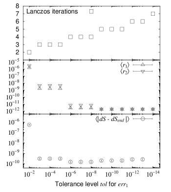
Figure 11: The convergence behavior of the Lanczos-based algorithm for $dS$ calculation as a function of the tolerance level. Upper figure shows the number of iteration in the Lanczos algorithm, middle one shows the residuals defined in Eqs. (7.5) and (7.6) for $(W[\hat{D}_{oo}])^{N_{f}/8}$ and ${(W[\hat{D}_{oo}^{\prime}])}^{-N_{f}/4}$, bottom one for the $|dS-dS_{\mathit{end}}|$ where $dS_{\mathit{end}}$ is the value of $dS$ itself at $\mathit{tol}=10^{-14}$.

7.3 Results on the large size lattice

We show the results on the large size lattice in Table 2. We quote the averaged plaquette value with the $R$-algorithm from Ref. [32]. We observe a roughly $2\sigma$ deviation, which may be ascribed to a finite step size error inherent in the $R$-algorithm. The number of multiplication of hopping matrices $M_{eo}$ and $M_{oe}$ measured in the program is roughly proportional to $N_{\mathrm{poly}}$, which is expected from the discussion in section 6. We will discuss the finite step size error of the $R$-algorithm and compare the computational cost of the PHMC algorithm to that of the $R$-algorithm after describing the numerical property of the reversibility violation, the Lanczos algorithm, and $dS$ for the PHMC algorithm.

As described in section 4, we investigate the reversibility violation on the large size lattice using the following observables:

$$\Delta H/H \equiv |H(t_{r}-t_{r})-H(0)|/H(0),$$ (7.1)

$$\Delta U \equiv \sqrt{\sum_{n,\mu,a,b}\left|(U_{\mu})_{a,b}(n)(t_{r}-t_{r})-(U_{\mu})_{a,b}(n)(0)\right|},$$ (7.2)

$$\Delta P \equiv \sqrt{\sum_{n,\mu,a,b}\left|(P_{\mu})_{a,b}(n)(t_{r}-t_{r})-(P_{\mu})_{a,b}(n)(0)\right|},$$ (7.3)

where $X(0)$ means the observable $X$ calculated at the initial configuration at $t=0$ in the MD evolution and $X(t_{r}-t_{r})$ the observable calculated at the reversed configuration which is obtained from the initial configuration at $t=0$ by integrating the MD equation to $t=t_{r}$ and then integrating back to $t=0$. The trajectory length is $t_{r}=1$. We measured these quantities using 20 configurations which are separated by 5 trajectories. We observe

$$\langle\Delta H/H\rangle = 0.26(6)\times 10^{-15},$$

$$\langle\Delta P\rangle/\sqrt{9\times 4\times N_{\mathrm{vol}}} = 0.4162(7)\times 10^{-14},$$

$$\langle\Delta U\rangle/\sqrt{9\times 4\times N_{\mathrm{vol}}} = 0.1484(2)\times 10^{-14},$$ (7.4)

with the $N_{\mathrm{poly}}=300$ PHMC algorithm. The errors are estimated with the binned jackknife method. These values are at a completely satisfactory level with the double precision arithmetic. Consequently it is concluded that the method we employed for the force calculation of the polynomial pseudo-fermion is stable in the MD evolution and does not cause violation of reversibility.

The validity of the CG based stopping criterion for the Lanczos method to calculate $dS$ in the noisy Metropolis test is also investigated on the same 20 configurations. We measured $dS$, and two residuals defined by

$$r_{1} = \left|\left((W[\hat{D}_{oo}])^{N_{f}/8}\right)^{8/N_{f}}\eta_{o}-W[\hat{D}_{oo}]\eta_{o}\right|/|W[\hat{D}_{oo}]\eta_{o}|,$$ (7.5)

$$r_{2} = \left|W[\hat{D}_{oo}^{\prime}]\left((W[\hat{D}_{oo}^{\prime}])^{-N_{f}/4}\right)^{4/N_{f}}\zeta_{o}-\zeta_{o}\right|/|\zeta_{o}|,$$ (7.6)

where $\zeta_{o}$ is defined in Eq. (5.3), and the number of iteration of the Lanczos iteration by varying the tolerance level $\mathit{tol}$ for $err_{1}$.

Figure 11 shows the convergence behavior of the above quantities. The number of iteration increases step by step with the decreasing stopping condition (top of the figure). The residuals Eqs. (7.5) and (7.6) stagnate around a $O(10^{-12})$ level (middle of the figure). As the residuals are defined as relative error, one may suspect that the number of $O(10^{-12})$ is not sufficient with the double precision arithmetic. We think this is due to the accumulation of round-off errors in applying the Lanczos iteration several times to calculate the residuals. Namely, for the explicit residual calculation, we need four times application of the Lanczos iteration for $r_{1}$ and twice for $r_{2}$ in the $N_{f}=2$ case, and the Lanczos iteration does not span the completely same Krylov subspace in each application.

For the correctness of the algorithm, $dS$ itself is more important. To see the stopping condition dependence of $dS$, we measured the convergence of $|dS-dS_{end}|$ as the metric and show the result in the bottom of Figure 11, where $dS_{end}$ is $dS$ at the most stringent stopping condition $\mathit{tol}=10^{-14}$. Since the change is too rapid against the change of the number of iteration, we could not see the exponential decay. The metric stagnates around $O(10^{-10})$. The reason is understood as follows. $dS$ is defined as the difference of $\zeta^{{\dagger}}_{o}W[\hat{D}_{oo}^{\prime}]^{-N_{f}/4}\zeta_{o}$ and $|\eta_{o}|^{2}$ in Eq. (5.3). Numerically it is observed that $\zeta^{{\dagger}}_{o}W[\hat{D}_{oo}^{\prime}]^{-N_{f}/4}\zeta_{o}$ and $|\eta_{o}|^{2}$. have almost the same values of about $3\times 16^{4}/2\sim O(10^{5})$, and the resulting $dS$ is of $O(10^{-1})$. Within double precision arithmetic, the subtraction of $O(10^{5})$ from $O(10^{5})$ yielding $O(10^{-1})$ for $dS$ means that $dS$ only has 9-10 significant figures. The stagnation around $O(10^{-10})$ would occur in such a case. We stress that the 9-10 significant figures for $dS$ is sufficient in the realistic simulations with $O(10^{4})$ trajectories. No visible effect from the choice of the CG-based stopping criterion is observed.

The plaquette value of the $R$-algorithm from Ref. [32] is larger than that of the PHMC algorithm about $2\sigma$ as shown in Table 2. This may contradict the previous observation on the small size lattice where the plaquette value of the $R$-algorithm approaches the value of the PHMC algorithm from smaller value. To make clear the $dt$ dependence of the plaquette with the $R$-algorithm, we imported the program of the $R$-algorithm into SR8000-F1 model and produced several trajectories with the $R$-algorithm on the large size lattice.

Table 3: The results with the $R$-algorithm on the large size lattice ($16^{4},\beta=5.7,am=0.02$). $\mathit{res}$ is used for the stopping criterion of the CG algorithm in the $R$-algorithm.

$\mathit{res}$	$10^{-4}$	$10^{-4}$	$10^{-4}$	$10^{-4}$
$[dt,N_{\mathrm{MD}}]$	[0.005,200]	[0.01,100]	[0.02,50]	[0.025,40]
# of Traj.	800	1200	1200	1000
#Mult/traj	113210(450)	56700(355)	28627(113)	23102(76)
$\langle P\rangle$	0.577102(63)	0.577133(67)	0.577194(71)	0.577294(67)
$\mathit{res}$	$10^{-4}$	$10^{-4}$	$10^{-4}$	$10^{-8}$
$[dt,N_{\mathrm{MD}}]$	[0.04,25]	[0.05,20]	[0.0625,16]	[0.02,50]
# of Traj.	1500	2000	2500	1000
#Mult/traj	14432(130)	11808(42)	9478(91)	77880(807)
$\langle P\rangle$	0.577389(71)	0.577076(100)	0.576423(232)	0.577411(67)
$\mathit{res}$	$10^{-12}$	$10^{-15}$	-	-
$[dt,N_{\mathrm{MD}}]$	[0.02,50]	[0.02,50]	-	-
# of Traj.	1000	800	-	-
#Mult/traj	127772(1162)	166573(424)	-	-
$\langle P\rangle$	0.577335(63)	0.577242(57)	-	-

Table 3 shows the results with the $R$-algorithm on the large size lattice. The definition of the norm $\mathit{res}$ for the stopping criterion of the CG algorithm required in the $R$-algorithm is the same as that of Ref. [32] (where the symbol $r$ is used instead of $\mathit{res}$). We do not observe clear stopping criterion dependence on $\langle P\rangle$. Figure 12 shows the $dt$ dependence of $\langle P\rangle$ on the large size lattice. Open circles are the results with the $R$-algorithm produced for the comparison. Filled square is the previous result with the $R$-algorithm [32]. Open triangles are the results with the PHMC algorithm scatted around $dt=0.02$ for clarity of presentation. We observe that the $dt$ behavior of the $R$-algorithm in small $dt$ region is slightly different from that of the small size lattice (Fig. 8), while the behavior at large $dt$ region is similar to each other. We also observe that the value of $dt$ where $\langle P\rangle$ largely deviate from the value at the limit $dt\rightarrow 0$ is different (it is $dt\sim 0.01$ in Fig. 8 and $dt\sim 0.04-0.05$ in Fig. 12).

Although we cannot make clear statement on the discrepancy of $dt$ behavior between two lattice sizes, we can say that the $dt$ dependence is affected by the physical situation and parameters. The reason is as follows. The error analysis of the $R$-algorithm by $dt$ perturbation fails at large $dt$. More precisely it is said that the point where the perturbative analysis fails is governed by $dt/m$ with $m$ the lightest fermion mode in the $R$-algorithm [33]. We do not tune the input parameters for these two simulation sets. It is natural that the physical lightest fermion mode is different between the small and large size lattices. Thus we consider that this discrepancy comes from the different physical parameter and situation between the small and large size lattices and $\langle P\rangle$ with the $R$-algorithm at $dt=0.02$ is accidentally larger than that with the PHMC algorithm in the large size lattice. We stress that the result from the PHMC algorithm is consistent with the limit $dt\rightarrow 0$ of the results with the $R$-algorithm.

Figure 12: MD step size $dt$ dependence of the averaged plaquette on the large size lattice. The dotted curve shows the fit with $f(dt)=adt^{2}+bdt^{3}+c$ to open circles with the $R$-algorithm. Filled square is the result from Ref. [32].

The computational cost of the PHMC algorithm of $N_{\mathrm{poly}}=400$ is comparable to that of the $R$-algorithm with $\mathit{res}=10^{-8}$ at $dt=0.02$ in terms of #Mult/traj on the large size lattice. We need to take the limit $dt\rightarrow 0$ and use sufficiently small $\mathit{res}$ in the $R$-algorithm theoretically, which requires significantly large amount of computational cost for the $R$-algorithm. The actual computational time for the PHMC algorithm with $N_{\mathrm{poly}}=400$ on the large size lattice was measured as $136$ sec for unit trajectory with SR8000-F1 4-nodes (peak speed : 12$\times$4 GFlops, sustained speed : 3.5$\times$ 4 GFlops) and it is $120$ sec for the $R$-algorithm with $\mathit{res}=10^{-8}$ (sustained speed : 3.4$\times$ 4 GFlops) at $dt=0.02$. The same computational speed is achieved because both programs make use of the common subroutine for the hopping matrix multiplication. Thus we conclude that the PHMC algorithm works on the lattice size of $16^{4}$ with a quark mass $am=0.02$ corresponding to $m_{\mathrm{PS}}/m_{\mathrm{V}}\sim 0.69$ [32] within reasonable computational time and is applicable to realistic simulations. The advantage of exact algorithm is very clear in this situation.

8 Conclusion

In this paper, we have presented an exact algorithm for dynamical lattice QCD simulation with the KS fermions where single flavor quark is defined as the $1/4$ power of the KS fermion matrix. The algorithm is an extension of the polynomial Hybrid Monte Carlo (PHMC) algorithm in which the Hermitian polynomial approximation is applied to the fractional power of the KS fermion matrix. The Kennedy-Kuti noisy Metropolis test is incorporated to make the algorithm exact.

We introduced two types of polynomial approximations and corresponding PHMC algorithms. One algorithm approximates $\hat{D}_{oo}^{-N_{f}/8}$ with a single polynomial $P_{N_{\mathrm{poly}}}[\hat{D}_{oo}]$ (case A), and the other $\hat{D}_{oo}^{-N_{f}/4}$ with a squared polynomial $|Q_{N_{\mathrm{poly}}}[\hat{D}_{oo}]|^{2}$ (case B). For the noisy Metropolis test, we made use of a Lanczos-based Krylov subspace method to calculate the fractional power of the correction matrix. The efficiency of the two algorithms was estimated, and it was found that the latter (case B) had better performance than that of the former by a factor two.

We tested our algorithm (case B) using the Hermitian Chebyshev polynomial for the case of two-flavor QCD on three lattice sizes. Results on a small lattice of $8^{3}\times 4$ demonstrated that the algorithm works correctly, e.g., the averaged plaquette value agrees with that of the $R$-algorithm after extrapolation to the zero step size limit. We have also shown that our algorithm works on a moderately large lattice of size $16^{4}$, albeit for a rather heavy quark mass of $m_{\mathrm{VS}}/m_{\mathrm{V}}\sim 0.69$, within reasonable simulation costs compared to that of the $R$-algorithm.

There are several points that require improvements with our work. One of the points concerns the fact that the calculation of the polynomial coefficients in case B for splitting the original polynomial becomes progressively difficult toward lighter quark masses. While this is not a limitation of the PHMC algorithm itself, solutions should be found to solve this problem for future realistic simulations since the case A algorithm, which has no such problem, is expected to be twice slower than than the case B algorithm. Another point is that further improvement of the algorithm may be achieved by optimizing the polynomial approximation, and by combining the preconditioning technique and the polynomial approximation.

Anticipating progress on these fronts, we conclude that our algorithm provides an attractive method for dynamical KS fermion simulations for $2+1$-flavor QCD without systematic errors originating from the simulation algorithm.

References

- [1] SESAM Collaboration: N. Eicker et al., Phys. Rev. D 59 (1999) 014509.
- [2] SESAM-TL Collaboration: Th. Lippert et al., Nucl. Phys. B (Proc. Suppl.) 60A (1998) 311.
- [3] N. Eicker, Th. Lippert, B. Orth, and K. Schilling, Nucl. Phys. B (Proc. Suppl.) 106 (2002) 209.
- [4] CP-PACS Collaboration: A. Ali Khan et al., Phys. Rev. D 65 (2002) 054505.
- [5] UKQCD Collaboration: C. R. Allton et al., Phys. Rev. D 60 (1999) 034507; ibid. D 65 (2002) 054502.
- [6] JLQCD Collaboration: S. Aoki et al., Nucl. Phys. B (Proc. Suppl.) 94 (2001) 233; Nucl. Phys. B (Proc. Suppl.) 106 (2002) 224.
- [7] MILC Collaboration: C. Bernard et al., Nucl. Phys. B (Proc. Suppl.) 73 (1999) 198; Phys. Rev. D 64 (2001) 054506; hep-lat/0206016
- [8] S. Duane, A. D. Kennedy, J. J. Pendleton, and D. Roweth, Phys. Lett. B195 (1987) 216.
- [9] For a pedagogical introduction to the HMC algorithms, A. D. Kennedy, Parallel Comput. 25 (1999) 1311.
- [10] Ph. de Forcrand and T. Takaishi, Nucl. Phys. B (Proc. Suppl.) 53 (1997) 968.
- [11] R. Frezzotti and K. Jansen, Phys. Lett. B402 (1997) 328; Nucl. Phys. B 555 (1999) 395; ibid. 432.
- [12] T. Takaishi and Ph. de Forcrand, Int. J. Mod. Phys. C 13 (2002) 343; Nucl. Phys. B (Proc. Suppl.) 94 (2001) 818; in Non-Perturbative Methods and Lattice QCD, Guangzhou 2000, World Scientific (2001), p. 112 [hep-lat/0009024].
- [13] JLQCD collaboration: S. Aoki et al., Phys. Rev. D 65 (2002) 094507; Nucl. Phys. B (Proc. Suppl.) 106 (2002) 1079.
- [14] S. Gottlieb, W. Liu, D. Toussaint, R.L. Renken, and R.L. Sugar, Phys. Rev. D 35 (1987) 2531.
- [15] I. Horváth, A. D. Kennedy, and S. Sint, Nucl. Phys. B (Proc. Suppl.) 73 (1999) 834.
- [16] F. Knechtli and A. Hasenfratz, Phys. Rev. D 63 (2001) 114502; A. Hasenfratz and F. Knechtli, hep-lat/0203010; Nucl. Phys. B (Proc. Suppl.) 106 (2002) 1058; hep-lat/0106014; hep-lat/0105022.
- [17] A. D. Kennedy and J. Kuti, Phys. Rev. Lett. 54 (1985) 2473.
- [18] A. Boriçi and Ph. de Forcrand, Nucl. Phys. B 454 (1995) 645; A. Borrelli, Ph. de Forcrand, and A. Galli, Nucl. Phys. B 477 (1996) 809.
- [19] C. Alexandrou, A. Boriçi, A. Feo, Ph. de Forcrand, A. Galli, F. Jegerlehner, and T. Takaishi, Phys. Rev. D 60 (1999) 034504.
- [20] A. Boriçi, Phys. Lett. B453 (1999) 46; J. Comput. Phys. 162 (2000) 123; in Numerical Challenges in Lattice Quantum Chromodynamics, Wuppertal 1999, Springer (2000), p. 40 [hep-lat/0001019].
- [21] M. Lüscher, Nucl. Phys. B 418 (1994) 637.
- [22] Ph. de Forcrand, Nucl. Phys. B (Proc. Suppl.) 73 (1999) 822; C. Alexandrou, Ph. de Forcrand, M. D’Elia, and H. Panagopoulos, Phys. Rev. D 61 (2000) 074503; Nucl. Phys. B (Proc. Suppl.) 83-84 (2000) 765.
- [23] I. Montvay, Comput. Phys. Commun. 109 (1998) 144; in Numerical Challenges in Lattice Quantum Chromodynamics, Wuppertal 1999, Springer (2000), p. 153 [hep-lat/9911014]; hep-lat/9903029.
- [24] B. Bunk, Nucl. Phys. B (Proc. Suppl.) 63A-C (1998) 952.
- [25] T. Kalkreuter, Phys. Rev. D 51 (1995) 1305.
- [26] W. H. Press, S. A. Teukolsky, W. T. Vetterling, and B. P. Flannery, Numerical Recipes (Cambridge University Press, Cambridge, England, 1988).
- [27] B. Bunk, S. Elser, R. Frezzotti, and K. Jansen, Comput. Phys. Commun. 118 (1999) 95.
- [28] C. Liu, Nucl. Phys. B 554 (1999) 313.
- [29] For underlying idea of the Krylov subspace method to matrix functions, see e.g. H. A. van der Vorst, in Numerical Challenges in Lattice Quantum Chromodynamics, Wuppertal 1999, Springer (2000), p. 18.
- [30] For the connection between the Lanczos and conjugate gradient algorithms, see e.g. G. H. Golub and C. F. Van Loan, Matrix Computations (3rd edition, The Johns Hopkins University Press, Baltimore and London, 1996).
- [31] J. van den Eshof, A. Frommer, Th. Lippert, K. Schilling, and H. A. van der Vorst, Comput. Phys. Commun. 146 (2002) 203 [hep-lat/0202025].
- [32] M. Fukugita, N. Ishizuka, H. Mino, M. Okawa, and A. Ukawa, Phys. Rev. D 47 (1993) 4739.
- [33] M. A. Clark, B. Joó, and A. D. Kennedy, hep-lat/0209035.