EPHOU-02-003

July, 2002

Numerical study for the $c$-dependence of fractal
dimension in two-dimensional quantum gravity
Noboru Kawamoto and Kenji Yotsuji
Department of Physics, Faculty of Science
Hokkaido University
Sapporo, 060-0810, Japan

We numerically investigate the fractal structure of two-dimensional quantum gravity coupled to matter central charge $c$ for $-2\leq c\leq 1$. We reformulate $Q$-state Potts model into the model which can be identified as a weighted percolation cluster model and can make continuous change of $Q$, which relates $c$, on the dynamically triangulated lattice. The $c$-dependence of the critical coupling is measured from the percolation probability and susceptibility. The $c$-dependence of the string susceptibility of the quantum surface is evaluated and has very good agreement with the theoretical predictions. The $c$-dependence of the fractal dimension based on the finite size scaling hypothesis is measured and has excellent agreement with one of the theoretical predictions previously proposed except for the region near $c\approx 1$.

1 Introduction

It could probably be one of the most annoying questions: ”What is the observable of quantum gravity to check if the quantum theory of gravity is well defined ?” In two-dimensional quantum gravity the answer to this question is ready: ”The fractal dimension of the quantum surface is the well-defined observable which can be analytically and numerically calculated.”

The importance of the fractal nature of two-dimensional quantum gravity was first recognized by KPZ [1] where the critical exponent is recognized to represent the fractal structure of the two-dimensional quantum surface. It has, however, been recognized later that more direct observable to detect the quantum fractal nature of space time would be the Housdorff dimension, or fractal dimension [2, 3].

The serious numerical study to measure the fractal nature of two-dimensional quantum surface was initiated by Agistein and Migdal [4]. They have proceeded the direct measurements of the fractal dimension of two-dimensional quantum surface by proposing a recursive sampling argorithm for $c=0$ model but could not observe the fractal nature of the quantum gravity in two dimension. The size of the triangulation was not large enough to observe the fractal nature of the quantum surface of $c=0$ model. The first numerical confirmation of the fractal structure of two-dimensional quantum gravity was carried out by Kawamoto, Kazakov, Saeki and Watabiki by using the recursive sampling argorithm for $c=-2$ model[5]. In these numerical analyses the large size lattice triangulation (up to 5 million triangles) was necessary to confirm the fractal nature by the direct measurement of the fractal dimension. This numerical confirmation of the two-dimensional quantum space-time triggered wide varieties of numerical and analytic investigations of the fractal nature of two-dimensional quantum gravity.

There are three analytic derivations of the $c$-dependence of Housdorff dimension or fractal dimension of two-dimensional quantum gravity coupled to matter central charge $c$, by Distler, Hlousek and Kawai[2], Kawai and Ninomiya[3] and later by Watabiki, Kawamoto and Saeki[6]. It was, however, pointed out that the measured fractal dimension of $c=-2$ model is very close to the third formulae given by Watabiki et. al. [6]. In the meantime Kawai, Kawamoto, Mogami and Watabiki tried to understand the fractal nature of quantum gravity from the Matrix model point of view and succeeded to derive the transfer matrix of the quantum surface of two-dimensional pure gravity ($c=0$)[7]. The formulation made it possible to derive the fractal dimension of pure gravity to be exactly $d_{F}=4$ which is consistent with the value of the first and third formulae. This analytic investigation of the random surface triggered further analytic and numerical investigations of two-dimensional gravity[8, 9, 10, 11].

Baby universe idea was proposed and proved to be useful to calculate string susceptibility numerically[12, 13]. Then finite size scaling hypothesis was proposed later by being inspired by the analytic derivation of the two-point function of pure gravity[14]. The finite size scaling hypothesis made it possible to measure the fractal dimension very accurately. Using this formulation we made systematic and the most reliable numerical measurement of the fractal dimension for $c=-2$ model [15, 16]. Then the very accurately measured fractal dimension of $c=-2$ model perfectly agreed with the theoretical value of the third formula, $d_{F}=3.56\pm 0.04(\hbox{numerical})\simeq 3.561\cdots(\hbox{theoretical})$.

So far the numerical investigations of the fractal dimensions were carried out mainly for $c=-2$ and $c=0$ model and for several unitary series of conformal field theory[17] and several values in the region $c>1$[18].

Here in this article we investigate the systematic investigation on the $c$-dependence of the fractal dimension of two-dimensional quantum surface. For $c=-2,0$ analytic formulae by the help of matrix model was available while for the other continuous value of matter central charge it was not obvious how to formulate the models to be convenient for the numerical study of the fractal dimension. It has, however, been known that the continuos central charge dependence can be accommodated by $Q$-state Potts model on the flat lattice. Here in this paper we reformulate the $Q$-state Potts model into the model which is a generalization of percolation cluster model, weighted percolation cluster model[19, 20]. We formulate the model on the dynamically triangulated lattice and extend to take non-integer value $Q$ which is a function of $c$. By this model we can investigate $c$-dependence of the fractal nature of the two-dimensional quantum gravity coupled to matter central charge $c$. There have already been several calculations of critical indices of Ising model, three-state Potts models, and large $Q$ values of $Q$-state Potts model coupled to quantum gravity[21, 22].

This paper is organized as follows: In section 2 we summarize the analytic derivations of Hausdorff dimension and fractal dimension. In section 3 we explain the equivalence of Potts model and a weighted percolation cluster model which we call generalized Potts model. We then provide the definition of the generalized Potts model on the dynamically triangulated lattice. In section 4 we explain the details of the Metropolis argolism of the generalized Potts model. In section 5 numerical results of the $c$-dependence of critical coupling constant, string susceptibility, and fractal dimension are shown. Conclusions and discussions are given in the last section.

2 Analytic derivation of fractal dimension and previous numerical results

The fractal nature of the two-dimensional quantum gravity was first recognized by KPZ[1]. It was, however, not clear what kind of fractal it meant in the beginning. Serious analytic study on the fractal dimension of quantum gravity has been given by Distler, Hlousek and Kawai[2], and Kawai and Ninomiya[3] and later by Watabiki, Kawamoto and Saeki[6]. Here we summarize the analytic derivation of the fractal dimension.

In the derivation of the fractal dimension of two-dimensional quantum gravity coupled with matter central charge $c$, we use the formulation of Liouville theory in particular the formulation of conformal gauge given by DDK[23]. We first summarize the main results of the formulation.

Formally the continuum partition function for matter coupled to two dimensional gravity is given by

$$Z(A)\ =\ \int{\cal D}g~{}\ \delta\left(\int d^{2}x\sqrt{g}-A\right)~{}\,Z_{M}[g],$$ (2.1)

where $Z_{M}[g]$ is a matter part of the partition function with gravitational background and $A$ is the total area.

Reguralized counterpart of the above partition function by dynamical triangulation is

$$Z_{reg}(A)\ =\ \sum_{G}\ Z_{M}[G]\,\delta_{Na^{2},A}~{}~{}\sim\ Z_{M}[G_{0}],$$ (2.2)

where $N$ is the number of equilateral triangles and $a^{2}$ is the area of the triangle. $G$ denotes a triangulation and $G_{0}$ is the typical triangulation which we select from the huge set of triangulations. The last approximate equality in eq.(2.2) is valid up to the normalization factor and if the selection of the typical surface is carried out by a correct procedure. Since the path integration of the metric is carried out after the selection of the typical surface, $G_{0}$ carries the information of the quantum fluctuation of space time effectively.

Following David, Distler and Kawai (DDK)[23], we obtain the gauge fixed version of the two-dimensional gravity coupled to matter central charge $c$ with a conformal gauge $g_{\mu\nu}=\hat{g}_{\mu\nu}e^{\phi}$:

$$Z(A)\ =\ \int{\cal D}_{\hat{g}}\phi\Delta_{\rm{FP}}[\hat{g}]Z_{\rm M}[\hat{g}]\,\delta\left(\int d^{2}x\sqrt{\hat{g}}e^{\alpha_{1}\phi}-A\right)\,\exp\left(\frac{c-25}{48\pi}S_{\rm L}[\phi,\hat{g}]\right),$$ (2.3)

where $\Delta_{\rm{FP}}$ is the Fadeev Popov contribution. $S_{\rm L}[\phi,\hat{g}]$ is the Liouville term given by

$$S_{\rm L}[\phi,\hat{g}]\ =\ \int d^{2}x\sqrt{\hat{g}}\,\left(\,\frac{1}{2}\,\hat{g}^{\mu\nu}\partial_{\mu}\phi\partial_{\nu}\phi\,+\,\phi\hat{R}\,\right),$$ (2.4)

where we set the renormalized cosmological constant equal to zero for simplicity. $\alpha_{1}$ appeared in eq. (2.3) is obtained from the following general formula:

$$\alpha_{n}\ =\ \frac{25-c\,-\,\sqrt{(25-c)(25-c-24n)}}{12}.$$ (2.5)

DDK have shown that the primary conformal field of weight $n-1$ can be made Weyl invariant at the quantum level with a quantum correction:

$$\int d^{2}x\sqrt{\hat{g}}\,e^{\alpha_{n}\phi}\Phi_{n},$$ (2.6)

where $\Phi_{n}$ transforms as $\Phi_{n}\mid_{\hat{g}e^{\sigma}}=e^{(n-1)\sigma}\Phi_{n}\mid_{\hat{g}}$. The term $e^{\alpha_{1}\phi}$ in the delta function of eq. (2.3) is needed to keep the world sheet volume to be $A$ at the quantum level.

Let us define an expectation value of an observable $O(g)$ by

$$<O(g)>_{A}\ = \ Z(A)^{-1}\int{\cal D}_{\hat{g}}\phi\Delta_{\rm{FP}}[\hat{g}]Z_{\rm M}[\hat{g}]\delta\left(\int d^{2}x\sqrt{\hat{g}}\,e^{\alpha_{1}\phi}\,-\,A\right)\,$$

$$O(\hat{g},\phi)\,\exp\left(\frac{c-25}{48\pi}S_{\rm L}[\phi,\hat{g}]\right).$$

2.1 Housdorff dimension and fractal dimension

Here we define two types of critical exponents which specialize the fractal nature of the two dimensional random surface.

Let us first define an intrinsic area $A(r)$ of the random surface as a function of the mean square average size of the world sheet $<r^{2}>$ as viewed in the embedding space. We define Hausdorff dimension $d_{H}$ as

$$A(r)=(\sqrt{<r^{2}>})^{d_{H}}.$$ (2.8)

It should be noted that this definition of Hausdorff dimension refers to the embedded space.

Let us next define $N(r)$ as the number of lattice points or number of triangles inside $r$ steps from a marked site. A step on the original lattice is one link step of a triangle while a step on the dual lattice is one dual link (edge) step on the dual lattice. We define fractal dimension $d_{F}$ as

$$N(r)=r^{d_{F}}.$$ (2.9)

This definition of the fractal dimension characterizes the connectivity of the random surface, how the random surface is composed by the connection of triangles, and thus could be called connectivity dimension.

Distler, Hlousek and Kawai[2] evaluated the mean square size of the quantum surface embedded in a $D$ dimensional space by calculating the two-point Green’s function of vertex operator

$$\frac{1}{D}<x^{2}>_{A}\ = \ 2\left|\frac{\partial}{\partial k^{2}}ln\left\langle\int d^{2}x_{1}\sqrt{\hat{g}(x_{1})}\int d^{2}x_{2}\sqrt{\hat{g}(x_{2})}e^{ik(X(x_{1})-X(x_{2}))}\right\rangle_{A}\right|_{k=0}$$ (2.10)

$$= \ \frac{1}{A^{2}Z(A)}\left\langle\int d^{2}x_{1}\sqrt{\hat{g}(x_{1})}\int d^{2}x_{2}\sqrt{\hat{g}(x_{2})}(X(x_{1})-X(x_{2}))^{2}\right\rangle_{A}$$

$$= \ \left(\frac{A}{A_{0}}\right)^{\mid\gamma_{s}\mid}\hskip 28.45274pt(A\rightarrow\infty),$$

where $\gamma_{s}$ is the string susceptibility given by

$$\gamma_{s}\ =\ \frac{D-1\,-\,\sqrt{(25-D)(1-D)}}{12}.$$ (2.11)

We can then obtain the first formula of Housdorff dimension as a function of $D$.

$$d_{H}^{(1)}\ =\ \frac{2}{\mid\gamma_{s}\mid},$$ (2.12)

where $D$ could later be identified as matter central charge $c$ in two dimension.

Let us next consider a derivation of fractal dimension using fermion as a test particle in the gravitational background following by Kawai and Ninomiya[3]. The Lagrangian for matter fermion coupled to gravity can be given by

$$L\ =\ -\frac{1}{16\pi}\sqrt{g}R\ +\ \Lambda\sqrt{g}\ +\ e\bar{\psi}i\not{\!\!D}\psi\ -\ me\bar{\psi}\psi,$$ (2.13)

where $\Lambda$ and $e$ are, respectively, cosmological constant and the determinant of the vielbein in $D$-dimensions. In $D=2+\epsilon$ dimensions gravitational quantum corrections can be evaluated by the $\epsilon$-expansion formulation[8]. Then the fermion mass term is expected to acquire anomalous dimension via wave function renormalization of the matter fermion.

Here we try to identify the anomalous dimension of the fermion mass term by the use of DDK formulation for Liouville theory. Under the scaling of the cosmological constant

$$\Lambda\ \rightarrow\beta^{-D}\Lambda,$$ (2.14)

the change in the Lagrangian can be absorbed by the field redefinition

$$g_{\mu\nu}\ \rightarrow\ \beta^{2}g_{\mu\nu}.$$ (2.15)

Since the vielbein transforms like square root of metric, the fermion kinetic term transforms as $e\bar{\psi}i\not{\!\!D}\psi\rightarrow\beta^{D-1}e\bar{\psi}i\not{\!\!D}\psi$. Then the scaling parameter can be absorbed by the field redefinition $\psi\rightarrow\beta^{(1-D)/2}\psi$. The fermion mass term changes as $me\bar{\psi}\psi\rightarrow\beta me\bar{\psi}\psi$, in particular $\bar{\psi}\psi\rightarrow\beta^{-1}\bar{\psi}\psi$ in $D=2$.

In two dimensions the fermion mass term $m\int d^{2}xe\bar{\psi}\psi$ is expected to have the form of eq. (2.6) after the introduction of the gravitational quantum correction. Since $\sqrt{g}$ and $e$ acquire the same scale change, $\bar{\psi}\psi$ can be identified as primary conformal field of $\Phi_{1/2}$ because of the same scale change: $\Phi_{1/2}\mid_{\hat{g}\beta^{2}}=\beta^{-1}\Phi_{1/2}\mid_{\hat{g}}$ and $\bar{\psi}\psi\rightarrow\beta^{-1}\bar{\psi}\psi$. Then the Weyl invariant fermion mass term with the quantum correction is given by

$$m\int d^{2}x\,\hat{e}\,e^{\alpha_{1/2}\phi}\,\bar{\psi}\psi.$$ (2.16)

We now consider the following quantum average of the fermion mass term:

$$m\left\langle\int d^{2}x\,\hat{e}\,e^{\alpha_{1/2}\phi}\,\bar{\psi}\psi\right\rangle_{A},$$ (2.17)

where the quantum average $<..>_{A}$ is defined in eq. (2). Under the constant shift of the conformal field $\phi\rightarrow\phi-2ln\beta/\alpha_{1}$, the quantum average should be unchanged and yet the following relation holds:

$$m\left\langle\int d^{2}x\,\hat{e}\,e^{\alpha_{1/2}\phi}\,\bar{\psi}\psi\right\rangle_{A}\,=\,m\beta^{-2\frac{\alpha_{1/2}}{\alpha_{1}}}\left\langle\int d^{2}x\,\hat{e}\,e^{\alpha_{1/2}\phi}\,\bar{\psi}\psi\right\rangle_{\beta^{2}A},$$ (2.18)

where the following change of delta function is taken into account:
$\delta\left(\int d^{2}x\sqrt{\hat{g}}\,e^{\alpha_{1}\phi}\,-\,A\right)\,\rightarrow\,\beta^{2}\delta\left(\int d^{2}x\sqrt{\hat{g}}\,e^{\alpha_{1}\phi}\,-\,\beta^{2}A\right)$. This relation suggests that the theory with two different sets of parameters $(A,m)$ and $\left(\beta^{2}A,m\beta^{-2\frac{\alpha_{1/2}}{\alpha_{1}}}\right)$ are equivalent. The two dimensional volume measured by the length scale of the fermion field leads to another definition of fractal dimension $d_{F}^{(2)}$ [3],

$$A\,\sim\,L^{2}\,=\,\left(L^{2\frac{\alpha_{1/2}}{\alpha_{1}}}\right)^{d_{F}^{(2)}},$$ (2.19)

where

$$d_{F}^{(2)}(c)\,=\,\frac{\alpha_{1}}{\alpha_{1/2}}\,=\,2\times{\sqrt{25-c}\,+\,\sqrt{13-c}\over\sqrt{25-c}\,+\,\sqrt{1-c}},$$ (2.20)

with $\alpha_{n}$ given by the formula (2.5).

2.2 Fractal dimension from diffusion equation of random walk

Here we provide yet another derivation of the fractal dimension by using the solution of diffusion equation on the random surface.

We define the laplacian on the dynamically triangulated lattice. We first define adjacency matrix $K_{ij}$ on the dynamically triangulated lattice. For a chosen typical surface $G_{0}$ we number the sites of the triangulated lattice. Then the ($i,j$) component of the adjacency matrix $K_{ij}$ is defined as: $K_{ij}=1$ if $i$-th site and $j$-th site are connected by a link, $K_{ij}=0$ if they are not connected by a link. It is interesting to note that ($n,n_{0}$) component of $(K^{T})_{i,j}$ counts the number of possible random walks reaching from a marking site $n_{0}$ to a site $n$ after $T$ steps. The Laplacian defined on the dynamically triangulated lattice is given by

$$\Delta_{L}\ =\ 1\,-\,S,~{}~{}~{}~{}~{}S_{ij}\ =\ {1\over q_{j}}K_{ij},$$ (2.21)

where $q_{j}$ is called coordination number and denotes a number of links connected to the site $j$. $S_{ij}$ is thus a probability of one step random walk from the site $j$ to the neighboring site $i$. The diffusion equation on a triangulated surface $G_{0}$ with $N$ triangles is given by

$$\partial_{T}\Psi_{N}^{(G_{0})}(T;n,n_{0})\ =\ \Delta_{L}(G_{0})\,\Psi_{N}^{(G_{0})}(T;n,n_{0}),$$ (2.22)

where $\partial_{T}$ is a difference operator in $T$ and $\Psi_{N}^{(G_{0})}(T;n,n_{0})$ is a wave function of the diffusion equation and denotes the probability of finding the random walker at the site $n$ after $T$ steps from the starting site $n_{0}$. A solution of the diffusion equation can be obtained as $\Psi_{N}^{(G_{0})}(T;n,n_{0})=e^{T\Delta_{L}(G_{0})}(\delta_{n,n_{0}})$, where $(\delta_{n,n_{0}})$ is $N$-component vector with unit $n_{0}$ entry.

We now consider the continuum limit of this diffusion equation. First of all we recover the lattice constant $a$. In taking continuum limit, the total physical area $A=a_{i}^{2}N_{i}$ is fixed and $i\rightarrow\infty;a_{i}\rightarrow 0,N_{i}\rightarrow\infty$ is taken, where $N_{i}$ is the number of triangles and $a_{i}^{2}$ is the area of a triangle. In each step of the limiting process we select a typical surface $G_{i}$ for the given number of triangles $N_{i}$, on which the lattice Laplacian $\Delta_{L}(G_{i})$ of eq.(2.21) is defined. Now the lattice version of the diffusion equation (2.22) can be rewritten by

$${1\over a_{i}^{2}}\{\Psi_{A}^{(G_{i})}(T+a_{i}^{2};x,x_{0})\,-\,\Psi_{A}^{(G_{i})}(T;x,x_{0})\}\ =\ {1\over a_{i}^{2}}\Delta_{L}(G_{i})\Psi_{A}^{(G_{i})}(T;x,x_{0})\},$$ (2.23)

where the location of the site $x$ is measured with respect to the lattice constant $a_{i}$. Thus we identify the dimension of $T$ as that of area: $dim[T]=dim[A]$. In the continuum limit the solution of the diffusion equation (2.23) is expected to approach the continuum wave function: $\Psi_{A}^{(G_{i})}(T;x,x_{0})\rightarrow\Psi_{A}^{(G_{\infty})}(T;x,x_{0})$. Numerically we approximate the limiting surface as the typical surface($G_{0}$) of the maximum size triangulation: $G_{\infty}\simeq G_{0}$. As we have already noted in eq.(2.2), the metric integration is effectively carried out for the equation (2.23) since we have chosen a typical surface. This means that the quantum effect is included for the wave function of eq.(2.23). On the other hand the solution of the continuum counterpart of the diffusion equation: $\partial_{\tau}\Psi(\tau;x,x_{0})=\Delta(g)\Psi(\tau;x,x_{0})$ is still background metric dependent in general. Furthermore the dimensions of $T$ and $\tau$ may not necessarily be equal.

Let us now define the comeback probability of random walk on the triangulated lattice and relate it with the continuum expression of Liouville theory as follows:

$$G(T)\ \equiv \ \Psi_{A}^{(G_{0})}(T;x=x_{0})\$$ (2.24)

$$\simeq \left.\ \left\langle\int d^{2}x\sqrt{g}\,\Psi(\tau;x=x_{0})\right\rangle_{A}\right/\left\langle\int d^{2}x\sqrt{g}\right\rangle_{A}\$$

$$= \ \frac{1}{A}\left\langle\int d^{2}x\sqrt{g}\,e^{\tau\Delta}\,\Psi(0;x=x_{0})\right\rangle_{A}\$$

$$\sim \ \frac{1}{A}\ \sim\ \frac{1}{T},$$

where $<..>_{A}$ is the quantum average defined in eq.(2) and the last similarity relations are dimensional relations. We should remind of the fact that the metric integration is effectively carried out since we have chosen the typical surface $G_{0}$ for the wave function of the comeback probability. The initial wave function can be formally written as $\Psi(0;x=x_{0})=\lim_{x\rightarrow x_{0}}\delta_{\epsilon}(x-x_{0})1/\sqrt{g}$, where the regularized delta function is needed such as: $\delta_{\epsilon}(x-x_{0})=(1/\pi)\times\epsilon/((x-x_{0})^{2}+\epsilon^{2})$.

We next consider how to accommodate the Weyl invariance into the diffusion equation of random walk at the quantum level by using the formulation of Liouville theory. Let us consider the following quantity by Liouville theory:

$$\left\langle\int d^{2}x\sqrt{g}\,\Psi(\tau;x=x_{0})\right\rangle_{A}$$

$$= \ \left\langle\int d^{2}x\sqrt{g}\,\Psi(0;x=x_{0})\right\rangle_{A}\ +\ \tau\,\left\langle\int d^{2}x\sqrt{g}\,\Delta\,\Psi(0;x=x_{0})\right\rangle_{A}\ +\ \cdots,$$

where the solution of the diffusion equation is expanded by $\tau$.
Taking a conformal gauge $g_{\mu\nu}(x)=\hat{g}_{\mu\nu}e^{\phi(x)}$ and introducing DDK arguments, we can rewrite the first and second terms of the eq.(2.2 ) as

$$\left\langle\int d^{2}x\sqrt{g}\,\Psi(0;x=x_{0})\right\rangle_{A}\ = \ \left\langle\int d^{2}x\sqrt{\hat{g}}\,\big{[}\frac{1}{\sqrt{\hat{g}}}\delta_{\epsilon}(x-x_{0})\big{]}_{x=x_{0}}\right\rangle_{A}\ =\ 1,$$

$$\left\langle\int d^{2}x\sqrt{g}\,\Delta\,\Psi(0;x=x_{0})\right\rangle_{A}\ = \ \left\langle\int d^{2}x\sqrt{\hat{g}}\,e^{\alpha_{-1}\phi}\,\big{[}\overrightarrow{\hat{\Delta}_{x}}\,\frac{1}{\sqrt{\hat{g}}}\delta_{\epsilon}(x-x_{0})\big{]}_{x=x_{0}}\right\rangle_{A},$$

where the term $e^{\alpha_{-1}\phi}$ is introduced to keep the Weyl invariance of the second line of eq.(2.2) in accordance with the arguments of eq. (2.6 ). Here it should be noted that $\Delta\,\Psi(0;x=x_{0})$ in the second term of eq. (2.2) can be identified as a primary conformal field of $\Phi_{-1}$.

Similar to the treatment for the Weyl invariance of the fermion mass term of eq. (2.18), the quantum average of the comeback probability should be unchanged under the constant shift of the conformal field $\phi\rightarrow\phi-2ln\beta/\alpha_{1}$. In particular the second term of eq.(2.2) should be unchanged and yet the following parameter change is generated:

$$\tau\left\langle\int d^{2}x\,\sqrt{\hat{g}}\,e^{\alpha_{-1}\phi}\,\hat{\Delta}\Psi(0;x=x_{0})\right\rangle_{A}\,=\,\tau\beta^{-2\frac{\alpha_{-1}}{\alpha_{1}}}\left\langle\int d^{2}x\,\sqrt{\hat{g}}\,e^{\alpha_{-1}\phi}\,\hat{\Delta}\Psi(0;x=x_{0})\right\rangle_{\beta^{2}A}.$$ (2.27)

This relation suggests that the theory with two different sets of parameters $(\tau,A)$ and $\left(\beta^{-2\frac{\alpha_{-1}}{\alpha_{1}}}\tau,\beta^{2}A\right)$ are equivalent. Then we obtain the following dimensional relation:

$$\hbox{\rm dim}{\tau}\ =\ \hbox{\rm dim}{A^{-\frac{\alpha_{-1}}{\alpha_{1}}}}.$$ (2.28)

We now point out that the expectation value of the mean squared geodesic distance is evaluated by the standard continuum treatment

$$\int d^{2}x\sqrt{g}\,\big{\{}r(x,x_{0})\big{\}}^{2}\,\Psi(\tau;x,x_{0})$$

$$= \ \int d^{2}x\sqrt{g}\,\big{\{}r(x,x_{0})\big{\}}^{2}\,\left(\frac{1}{\sqrt{\hat{g}}}\delta(x-x_{0})\,+\,\tau{\hat{\Delta}_{x}}\,\frac{1}{\sqrt{\hat{g}}}\delta(x-x_{0})\,+\cdots\right)$$

$$= \ -\,4\tau\ +\ O(\tau^{2}),$$ (2.29)

which is related to the quantum version of the mean squared geodesic distance in the small $\tau$ region

$$<r^{2}>$$ (2.30)

$$\equiv \ \sum_{x}\,\{r(x,x_{0})\}^{2}\,\Psi_{A}^{(G_{0})}(T;x,x_{0})$$

$$\simeq \left.\left\langle\int d^{2}x\sqrt{g}\,\int d^{2}x_{0}\sqrt{g}\,\{r(x,x_{0})\}^{2}\,\Psi(\tau;x,x_{0})\right\rangle_{A}\right/\left\langle\int d^{2}x\sqrt{g}\right\rangle_{A}\$$

$$\sim \ \tau\ \sim\ A^{-\frac{\alpha_{-1}}{\alpha_{1}}}\ \sim\ T^{-\frac{\alpha_{-1}}{\alpha_{1}}}.$$

The last similarity relations are dimensional relations. Here we give the third definition of fractal dimension

$$A\,=\,\left(\sqrt{<r^{2}>}\right)^{d_{F}^{(3)}}$$ (2.31)

where

$$d_{F}^{(3)}(c)\ =\ -\,2\,\frac{\alpha_{1}}{\alpha_{-1}}\ =\ 2\times\frac{\sqrt{25-c}\,+\,\sqrt{49-c}}{\sqrt{25-c}\,+\,\sqrt{1-c}},$$ (2.32)

with $\alpha_{n}$ given by eq. (2.5).

2.3 Previous numerical results

Serious numerical investigations of the fractal nature of two-dimensional quantum gravity ($c=0$ model) was initiated by Agistein and Migdal for $c=0$ model[4]. They proposed recursive sampling algorithm which partially use an analytic formula for tree diagrams and rainbow diagrams to generate planar Feynman diagrams corresponding to different types of two-dimensional sphere. They could’t, however, observe the fractal structure numerically for this model. The fractal nature of two-dimensional quantum gravity was numerically first confirmed by Kawamoto, Kazakov, Saeki and Watabiki by using the recursive sampling algorithm for $c=-2$ model[5]. It was recognized in this numerical analyses that large number of triangles is necessary to confirm the fractal nature by the parameterization of the fractal dimension given by (2.9). In fact they needed 5 million triangles to confirm the fractal nature. It was then recognized that the number of triangles were not large enough to measure the fractal dimension of $c=0$ model.

The numerical fractal dimension of $c=-2$ model was given in this numerical analyses as $d_{F}\simeq 3.55$. After deriving the third formula of the fractal dimension $d_{F}^{(3)}(c)$ of eq.(2.32), we have recognized that the numerical value of the fractal dimension is close to the theoretical value of the third formula $d_{F}^{(3)}(-2)=(3+\sqrt{17})/2=3.561\cdots$.

Except for the analytic derivation of the fractal dimension, one obtains the following analytic relations of comeback probability in (2.24) and mean squared geodesic distance in (2.30) from the diffusion equation:

1. (1) $G(T)T\ \sim\ const.$,

2. (2) $<r^{2}>\ =\ T^{{2}/{d_{F}^{(3)}(-2)}}\ \simeq\ T^{-0.56}$,
   

which can be numerically checked. These relations were numerically confirmed for $c=-2$ model in [6].

An alternative analytic investigation of the fractal structure of the pure gravity ($c=0$) were carried out by deriving transfer matrix of random surface by Kawai, Kawamoto, Mogami and Watabiki. They found out the beautiful scaling function $\rho(L;D)$ which counts the number of boundaries whose boundary lengths lie between $L$ and $L+dL$ located at geodesic distance $D$ measured from a marked point. It is evaluated by taking the continuum limit from the transfer matrix and disk amplitude of dynamical triangulation. The functional form of $\rho(L;D)$ for $c=0$ model is given by

$$\rho(L;D)D^{2}\ =\ {3\over 7\sqrt{\pi}}(x^{-5/2}+{1\over 2}x^{-3/2}+{14\over 3}x^{1/2})e^{-x},$$ (2.33)

where $x=L/D^{2}$ is a scaling parameter. This quantity $\rho(L;D)D^{2}$ for $c=0$ model was measured numerically and had excellent agreement with the theoretical scaling function (2.33)[11]. One of the important result of this analysis is that the fractal dimension of the $c=0$ model turns out to be $d_{F}=4$ which is consistent with the first and third formulae.

Based on these theoretical and numerical evidences the third formula of the fractal dimension would be the correct formula for the $c$-dependence of the fractal dimension. In order to clear up the situation we started serious systematic and very accurate numerical study of $c=-2$ model by using finite size scaling hypothesis[15, 16]. It was concluded that the measured fractal dimension from this analysis is $d_{F}=3.56\pm 0.04$ which is perfectly consistent with the theoretical value of the third formula.

3 Generalized Potts model $\equiv$ Weighted percolation cluster model

Potts model [19] was defined as a generalization of the Ising model [25]. Fortuin and Kasteleyn [20] showed that the $Q$-state Potts model is equivalent to a weighted percolation cluster model which we explain in this section. Their construction allows the Potts model to be generalized to nonintegral values of $Q$. We may call this model as generalized Potts model or equivalently weighted percolation cluster model. These models were originally formulated on the square lattice while we extend to formulate the model on a dynamically triangulated lattice.

We define a planar $\varphi^{3}$-graph ${\cal G}$ dual to a triangulated lattice. Let a graph ${\cal G}_{N}$ have $N$ vertices which are dual to triangles in the triangulated lattice. With each vertex $i$, we associate a spin that can take $Q$ different values $\sigma_{i}=1,2,\cdots,Q$. Two adjacent spins $\sigma_{i}$ and $\sigma_{j}$ interact with interaction energy $-J\,\delta(\sigma_{i},\sigma_{j})$, where

$$\delta(\sigma_{i},\sigma_{j})=\left\{\begin{array}[]{ll}1,&\quad\sigma_{i}=\sigma_{j}\\ 0,&\quad\sigma_{i}\neq\sigma_{j}~{}.\end{array}\right.$$ (3.1)

Thus the Hamiltonian is

$$H=-K\sum_{\langle i,j\rangle}\delta(\sigma_{i},\sigma_{j})\,,$$ (3.2)

where $K=J/k_{B}T$ can be reinterpreted as a coupling constant and the summation runs over all the pairs of nearest-neighbor vertices $\langle i,j\rangle$. Then the partition function of this model is given by

$$Z_{N}(K;{\cal G}_{N})=\sum_{\{\sigma\}\,\mbox{{\scriptsize on}}\,{\cal G}_{N}}\exp\biggl{[}K\sum_{\langle i,j\rangle}\delta(\sigma_{i},\sigma_{j})\biggr{]}\,,$$ (3.3)

where the $\sigma$-summation runs over all possible values $\{\sigma_{i}=1,2,\cdots,Q\}$ for the spin variables $\sigma_{1},\sigma_{2},\cdots,\sigma_{N}$ on ${\cal G}_{N}$. Thus there are $Q^{N}$ terms in the summation.

It has been shown [20, 26] that the partition function (3.3) can be expressed as a dichromatic polynomial [27]. In order to see this, let us expand the partition function as a product of terms associated with nearest-neighbor vertices. This can be worked out by using the relation $[\delta(\sigma_{i},\sigma_{j})]^{m}=\delta(\sigma_{i},\sigma_{j})~{}(m=1,2,\cdots)$ as follows

$$Z_{N}(K;{\cal G}_{N})=\sum_{\{\sigma\}}\prod_{\langle i,j\rangle}\left[1+v\,\delta(\sigma_{i},\sigma_{j})\right]\,,$$ (3.4)

where we set $v=\exp(K)-1$.

Let $E$ be the number of the pairs of the nearest-neighbor vertices which we simply call edges on the graph ${\cal G}_{N}$. It is equal to the number of original links in the triangulated lattice, i.e. $3N/2$. Then the summand in eq.(3.4) is a product of $E$ factors. Each factor is the sum of two terms ($1$ and $v\,\delta(\sigma_{i},\sigma_{j})$), so the product can be expanded as the sum of $2^{E}$ terms. Each of these $2^{E}$ terms can be associated with a bond-cluster-graph (from now on call this a cluster configuration) on ${\cal G}_{N}$. Note that the term is a product of $E$ factors, one for each edge. The factor for edge $\langle i,j\rangle$ is either $1$ or $v\,\delta(\sigma_{i},\sigma_{j})$: if it is the former, leave the edge empty, if the latter, place a bond on the edge with weight $v\,\delta(\sigma_{i},\sigma_{j})$. Do this for all edges $\langle i,j\rangle$. We then have a one-to-one correspondence between cluster configurations on ${\cal G}_{N}$ and terms in the expansion of the product in eq.(3.4).

Consider a typical cluster configuration, containing $C$ connected components ($1\leq C\leq N$), namely, clusters and $b=\sum_{i=1}^{C}b_{i}$ bonds ($0\leq b\leq 3N/2$). See fig.1.

Figure 1: A fragment of a cluster configuration on a planar $\varphi^{3}$-graph. An isolated vertex is regarded as a cluster.

$i$-th cluster includes $b_{i}$ bands and an isolated vertex may be regarded as a cluster with $b_{i}=0$. Then the corresponding term in the expansion contains a factor $v^{b}$, and the effect of the delta functions is that all vertices within a component must have the same spin $\sigma$. Summing over independent spins, it follows that terms gives a contribution $Q^{C}v^{b}$ to the partition function $Z_{N}$. Summing over all such terms, i.e. over all cluster configurations, we have

$$Z_{N}^{Q}(K;{\cal G}_{N})=\sum_{{\scriptstyle\{cluster\}}\atop{\scriptstyle\mbox{{\scriptsize on}}~{}{\cal G}_{N}}}Q^{C}v^{b}\,.$$ (3.5)

The summation is over all cluster configurations that can be drawn on ${\cal G}_{N}$. The expression (3.5) is a dichromatic polynomial. Note that $Q$ in eq.(3.5) need not be an integer. We can allow it to be any positive real number, and this can be a useful generalization of $Q$-state Potts model to non-integer real number $Q$. We may call this model as generalized $Q$-state Potts model or weighted percolation cluster model.

Let us consider eq.(3.5) for a few particular values of $Q$. Firstly, we consider a model $Z_{N}^{Q=1}(K)$ formulated on a given triangulated lattice. For the $Q\to 1$ limit, if we set $v=p/(1-p)$ the partition function is

$$Z_{N}^{Q=1}(K) = \sum_{\{cluster\}}v^{b}$$ (3.6)

$$= \biggl{(}\frac{1}{1-p}\biggr{)}^{E}\sum_{\{cluster\}}p^{b}(1-p)^{E-b}\,.$$

Therefore, $Z_{N}^{Q=1}(K)$ becomes a sum over all possible bond percolation configurations with the correct weight where $p$ is the probability of a bond being present [20]. This result holds in any dimension and any lattice on which one defines the Potts models. Since the sum $\sum_{\{cluster\}}$ in eq.(3.6) is the total probability and thus equal to $1$, this model coupled to two-dimensional quantum gravity corresponds to the pure gravity model ($c=0$).

Next, let us examine for the $Q\to 0$ limit. At the critical point of the $Q$-state Potts model on the two-dimensional square lattice, it is known that $v\sim Q^{1/2}$ [19]. In general, on a graph ${\cal G}_{N}$ we can assume $v~{}\sim Q^{\alpha}$ in the $Q\to 0$ limit ($0<\alpha<1$). Then the partition function $Z_{N}^{Q\to 0}(K)$ becomes

$$Z_{N}^{Q\to 0}(K)~{}\sim~{}Q^{\alpha N}\sum_{\{cluster\}}Q^{\alpha l+(1-\alpha)C}\,,$$ (3.7)

where $l$ is the number of independent loops in a cluster configuration. We have used the Euler relation (See fig.1):

$$b=N+l-C\,.$$ (3.8)

For $0<\alpha<1$ the leading terms in eq.(3.7) in the $Q\to 0$ limit can be obtained by taking $C=1$ (one cluster) and $l=0$ (no loops). These dominant configurations are just the spanning trees of the graph ${\cal G}_{N}$ [20, 28]. Then each spanning tree configuration contributes to $Z_{N}^{Q\to 0}(K)$ with an equal weight. Therefore, this model coupled to two-dimensional quantum gravity is equivalent to the $c=-2$ scalar fermion model coupled to quantum gravity [5].

Temperley and Lieb [29] used the result of Fortuin and Kasteleyn to prove the equivalence of the Potts model to the six-vertex or square-ice model, with staggered polarizations. Baxter, Kelland and Wu (BKW) [26] have later found a very elegant derivation of the result of Temperley and Lieb. They use a construction known as the BKW construction which makes many exact results obvious, including the critical temperature, self-duality and energy at criticality of the Potts model.

Thus the $Q$-state Potts models are analytically solved and the relations with the conformal field theories are well known [30, 31]. $Q$ is related to central charge $c$ in the following particular form:

$$Q=4\cos^{2}\biggl{(}\frac{\pi}{m+1}\biggr{)},~{}~{}~{}~{}~{}~{}~{}~{}c=1-\frac{6}{m(m+1)}\,.$$ (3.9)

The minimal unitary conformal field theories with central charge $c$ between $0$ and $1$ correspond to integer $m$; $m=2,3,4,\cdots$. The generalization of $Q$ to any positive real number corresponds to a continuous change of the central charge $c$, a generalization from minimal to non-minimal series of conformal field theories.

Within the framework of dynamical triangulations the generalized Potts model, or equivalently the weighted percolation cluster models, coupled to two-dimensional quantum gravity is described by the following partition function:

$$Z_{N}^{Q}(K)=\sum_{{\cal G}_{N}\in\{\varphi^{3}(T_{N})\}}\frac{1}{{\cal S}_{{\cal G}_{N}}}\,\sum_{\{cluster\}}Q^{C}v^{b}\,.$$ (3.10)

where $\{\varphi^{3}(T_{N})\}$ denotes the set of $\varphi^{3}(T_{N})$-graphs dual to triangulations $T_{N}$ of fixed topology (which we always assume to be sphere) and ${\cal S}_{{\cal G}_{N}}$ is a symmetry factor.

4 The Metropolis algorithm of the generalized Potts model

We intend to evaluate numerically the fractal dimensions of two dimensional quantum gravity coupled to matter central charge $c$ by the generalized Potts model, equivalently the weighted percolation cluster model formulated in the previous section (3.10). In the process of Metropolis updating we need double step updating: firstly we update a cluster configuration on a given graph ${\cal G}_{N}$, secondly the graph ${\cal G}_{N}$ itself should be updated.

Here we first formulate the Metropolis algorithm of cluster configuration on a given graph ${\cal G}_{N}$. The equation (3.5) leads us to choose the probability distribution of the generalized Potts model for a cluster configuration $\{C\}_{k}$ by

$$P[\{C\}_{k}]\,=\,\frac{Q^{C^{(k)}}v^{b^{(k)}}}{Z_{N}^{Q}(K;{\cal G}_{N})},$$ (4.1)

where $C^{(k)}$ and $b^{(k)}$ are the number of cluster and the total number of edges $b^{(k)}=\sum_{i=1}^{C^{(k)}}b^{(k)}_{i}$ for the given cluster configuration $\{C\}_{k}$, respectively.

We need to define a transition function $t[\{C\}_{k},\{C\}_{l}]$ for a transition $\{C\}_{k}\to\{C\}_{l}$, which satisfies ergodicity and the following detailed balance condition:

$$P[\{C\}_{k}]\,\,t[\{C\}_{k},\{C\}_{l}]=P[\{C\}_{l}]\,\,t[\{C\}_{l},\{C\}_{k}]\,.$$ (4.2)

Here we choose to use Glauber function [32] as the transition function

$$t[\{C\}_{k},\{C\}_{l}]=\,\frac{\delta W_{lk}}{1+\delta W_{lk}}\,,$$ (4.3)

where

$$\frac{t[\{C\}_{k},\{C\}_{l}]}{t[\{C\}_{l},\{C\}_{k}]}=\,\delta W_{lk}=\,Q^{\delta C_{lk}}v^{\delta b_{lk}}$$ (4.4)

with $\delta C_{lk}=C^{(l)}-C^{(k)}$ and $\delta b_{lk}=b^{(l)}-b^{(k)}$.

For a given cluster configuration $\{C\}_{k}$, our updating proceeds as follows:

1. We randomly pick up an edge on the graph ${\cal G}_{N}$ and change the edge by the following procedure and then the cluster configuration changes into $\{C\}_{l}$.

2. We have to find out a change of the probability distribution $\delta W_{lk}=Q^{\delta C_{lk}}v^{\delta b_{lk}}$ when we change the edge, where $\delta b_{lk}$ is the change in the total number of bonds. If the edge originally has a bond, remove the bond thus $\delta b_{lk}=-1$. If the edge originally doesn’t have a bond, add a bond to the edge thus $\delta b_{lk}=+1$. $\delta C_{lk}$ is the change in the number of clusters depending on the corresponding change of the edge.

3. Next, we generate a pseudorandom number $r$ uniformly distributed from $0$ to $1$ and change the edge following to the procedure (2) if and only if

   $$r\leq\frac{\delta W_{lk}}{1+\delta W_{lk}}\,.$$ (4.5)

   This procedure ensures the transition $\{C\}_{k}\to\{C\}_{l}$ with the correct probability. We use the Glauber function for the transition function because of a faster convergence to the equilibrium distribution in our model.

4. Return to (1) unless the system is sufficiently equilibrated.

By this updating, ergodicity and detailed balance condition can be ensured.

Let us point out that it is nontrivial to evaluate $\delta C_{lk}$ in the step (2). For a given cluster configuration $\{C\}_{k}$, we pick up an edge on a graph ${\cal G}_{N}$. Suppose the edge does not have a bond we add a bond on the edge with the probability of the step (3) and thus $\delta b_{lk}=+1$ if the bond is added. For example we pick up the edge A-B which has vertices A and B in fig.2-(a) or the edge C-D which has vertices C and D in fig.2-(c), where those edges A-B and C-D does not have a bond. After the bond A-B and the bond C-D are added, (a) and (c) of fig.2 turn into (b) and (d) of fig.2, respectively. In order to find $\delta C_{lk}$ we need to know if the both vertices of the edge belong to the same cluster or not before the bond is added. For example the vertices A and B in fig.2-(a) belong to the different clusters while the vertices C and D in fig.2-(c) belong to the same cluster. It is not time consuming to classify this difference numerically since we just need to know the data set of the collection of numbered vertices belonging to the same cluster. If both vertices originally belong to the different clusters then $\delta C_{lk}=-1$, while $\delta C_{lk}=0$ if they originally belong to the same cluster. It is thus numerically not difficult to identify $\delta C_{lk}$ in the case of $\delta b_{lk}=+1$.

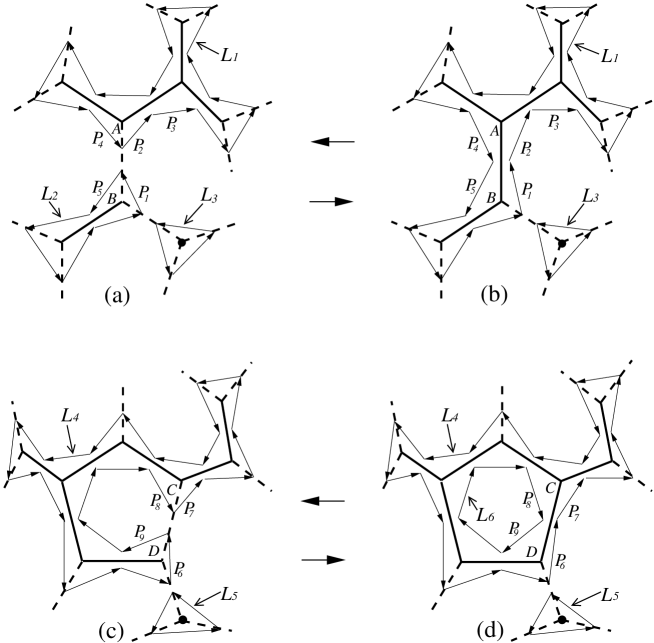
Figure 2: Cluster configurations: (a),(b),(c),(d). Doded lines are edges without bond while solid lines are edges with bond. A and B are vertices in (a) and (b) while C and D are vertices in (c) and (d). $L_{i}$ denotes i-th surrounding loop. The arrows are pointers and compose the segments of the surrounding loops.

Let us suppose that we pick up an edge which already has a bond. Then we remove the bond with the probability of the step (3) and thus $\delta b_{lk}=-1$ if it is removed. We may pick up cluster configurations (b) and (d) of fig.2 as particular examples which already has a bond at the edge A-B and C-D, respectively, and turn into (a) and (c) of fig.2, respectively, after the bond A-B and C-D are removed. In order to find $\delta C_{lk}$ we need to know the information if the both vertices of the edge belong to the same cluster or not after the bond is removed. The vertices A and B belong to the different cluster in (a) and thus $\delta C_{lk}=+1$, while the vertices C and D belong to the same cluster in (c) and thus $\delta C_{lk}=0$. The crucial difference from the case $\delta b_{lk}=+1$ to the case $\delta b_{lk}=-1$ is that the collection of the data set to classify the different cluster is not enough to differentiate if two vertices are in the same cluster or not after the bond is removed. The straightforward way to determine the connectedness of two vertices is to start from the first vertex and enumerate all vertices connected to it until either the second vertex is reached, or an entire connected region will be enumerated. This method is adequate if the clusters are small enough (tens of vertices), but if large clusters are involved (in the vicinity of the critical point) the CPU time requirements can grow unreasonable. Since the connectedness, a non-local property, must be determined with every iteration to know $\delta C_{lk}$, it is important to find faster algorithm to evaluate $\delta C_{lk}$. In order to quickly determine the connectedness of large clusters, we have implemented an algorithm [33] using an auxiliary data structure based on the BKW construction [26].

Let us reconsider a ${\varphi^{3}}$-graph ${\cal G}_{N}$, with $N$ vertices, together with its dual triangular lattice $T_{N}$. If a bond is present on ${\cal G}_{N}$, then its dual bond on $T_{N}$ is absent, and vice versa. The boundaries between clusters on ${\cal G}_{N}$ and their dual clusters on $T_{N}$ will form a collection of closed loops. Now we call this closed loops the surrounding loops. We then have the Euler relation,

$$b+2C=N+L\,,$$ (4.6)

which relates the number of clusters and bonds to the number of surrounding loops $L$.

By saving information of the surrounding loops as a data set, we transform the problem of determining connectedness of two vertices to the problem of determining whether two surrounding loop segments are part of the same surrounding loop or not. The surrounding loops are represented as a chain of pointers in the computer. A pointer is a memory location containing the address of the next pointer in the chain. There are three surrounding pointers represented by arrows for each vertex, as is shown in fig.3. We have shown surrounding loops composed of pointers for the figures (a), (b), (c), and (d) of fig.2. For example in fig.2-(b) pointer $P_{1}$ points to pointer $P_{2}$, $P_{2}$ points to $P_{3}$, etc. In this manner the loops are represented by chains of pointers. Because of the (differential) Euler relation, $\delta b_{lk}+2\delta C_{lk}=\delta L_{lk}$, we can determine $\delta C_{lk}$ if we can determine $\delta L_{lk}$, the change in the number of surrounding loops.

Figure 3: Three pointers surrounding each vertex.

Now, let us consider cases of removing a bond in the process of a Metropolis updating in Fig.2. The change; fig.2-(b) $\rightarrow$ fig.2-(a), illustrates the case in which removing the bond A-B will divide the surrounding loop $L_{1}$ into two surrounding loops $L_{1}$ and $L_{2}$ in fig.2-(a), while the change; fig.2-(d) $\rightarrow$ fig.2-(c), illustrates the case in which two surrounding loops $L_{4}$ and $L_{6}$ in fig.2-(d) will be joined into the loop $L_{4}$ in fig.2-(c) if the bond C-D is removed. In either case, two cuts must be made in chains of pointers and the four ends rejoined if the bond is removed. In the case of A-B bond in fig.2-(b), the $P_{1}\to P_{2}$ and the $P_{4}\to P_{5}$ connections must be replaced by $P_{1}\to P_{5}$ and $P_{4}\to P_{2}$ connections, respectively, in fig.2-(a). Similarly in the case of the bond C-D in fig.2-(d), the $P_{6}\to P_{7}$ and the $P_{8}\to P_{9}$ connections must be replaced by $P_{6}\to P_{9}$ and $P_{8}\to P_{7}$ connections, respectively, in fig.2-(c). By collecting the information of chains we can immediately conclude that $\delta C_{lk}=+1\,(\hbox{for}\,\delta b_{lk}=-1)$ since $P_{1}$ and $P_{4}$ are in the same chain for fig.2-(b) while $P_{6}$ and $P_{8}$ are in the different chains for fig.2-(d) and thus $\delta C_{lk}=0\,(\hbox{for}\,\delta b_{lk}=-1)$. It is important to note that the imformation of the connectedness of the cluster configuration of (a) and (c) can be obtained by the data set of the chains of pointers of (b) and (d), respectively. It is numerically much easier to find if two pointers are in the same loop chain or not.

In summary, in order to find $\delta W_{lk}$ for the Metropolis algorithm of the generalized Potts model in Monte Carlo simulation, we first pick up an edge and find out $\delta b_{lk}$ depending on whether the edge has a bond or not. We first cut and rejoin our chains of pointers depending on addition or removal of the bond on the edge. Using the (differential) Euler relation, $\delta b_{lk}+2\delta C_{lk}=\delta L_{lk}$, we evaluate $\delta C_{lk}$ by judging whether two pointers attached to the different vertices of the given edge belong to the same chain or not.

When we apply Monte Carlo simulations to quantum gravity coupled to the generalized Potts model or equivalently the weighted percolation clusters, we have to update the cluster configuration for a given triangulation and at the same time we have to update the triangulation for a given cluster configuration. The updating of cluster configurations on a given triangulation can be carried out just as described in the above. In order to update triangulations corresponding to the given $\varphi^{3}$- graphs ${\cal G}_{N}$, we use the standard flip-flop algorithm. We first choose two neighboring triangles randomly and flip the common link to generate a new triangulation. This flip move changes the triangulation locally as in fig.4. This move is enough to make the process ergodic for the chosen class of triangulations; fixed number of triangles and fixed topology [34].

Figure 4: The flip move. This move is ergodic in the class of triangulations with a fixed number of triangles and fixed topology.

In our simulations we avoid to generate configurations corresponding to tadpole and self-energy graphs. In other words we consider the class of triangulations satisfying the following conditions:

1. No link has coinciding end.

2. Two sites may be connected by no more than one link (i.e. parallel links are forbidden).

In the updating of triangulations, if a triangulation in a forbidden class is generated we ignore the attempt to make the flip and instead choose a new link randomly and attempt a new flip.

It is important to recognize that the flip procedure to generate random surface changes the cluster configuration. By the flip procedure the chosen edge which is the dual of the common link of the chosen neighboring triangles changes into a new edge which may or may not have a bond. In the present algorithm we generate a bond on the new edge with 50% probability. For example a cluster configuration in fig.5 changes into two possible cluster configurations with an equal probability by the flip procedure. In this way a change in connectivity of two triangles concerned with updating entails a change in the assignments of neighbors and therefore a change in the weight function $P[\{C\}_{k}]\,=\,Q^{C^{(k)}}v^{b^{(k)}}/Z_{N}^{Q}(K;{\cal G}_{N})$ and then the transition function, $\delta W_{lk}/(1+\delta W_{lk})$, can be estimated according to the Metropolis scheme described in the above.

Figure 5: Bond assignment after a flip move in a fragment of a cluster configuration. The bond is assigned to the new edge with 50 % probability.

5 Numerical simulations and results

The Monte Carlo simulations of generalized Potts models on dynamically triangulated surfaces are performed using the algorithm mentioned in the previous section. In our simulations we only generate planar $\varphi^{3}$-graphs of spherical topology with no tadpole or self-energy configurations. And we perform simulations on graphs with the fixed number $N$ vertices.

We first define one sweep of our Monte Carlo simulation. In the process of updating for a given cluster configuration with a fixed triangulation one cluster-sweep means checking of the Metropolis procedure on each edge of the graph in a given order. On the other hand, in the process of updating dynamical triangulation, one triangulation-sweep means that we randomly pick up edges one after another with roughly $3N/2$ (total number of edges) times and try to flip them and at the same time we check to eliminate every triangulations containing tadpole or self-energy graph.

After generating an initial cluster configuration, we thermalize our system by performing 2000 triangulation-sweeps and 1000 cluster-sweeps respectively. For the observables to be measured, this thermalization time is enough to thermalize our system according to the measurement of the autocorrelation time at criticality. To obtain a typical cluster sample configuration on a typical random surface background we perform 100 triangulation-sweeps and 20 cluster-sweeps. Then we measure several observables for the given configuration. We iterate these operations enough times until independent samples of a given number, which depends on the lattice size and on the observable to be measured, are obtained.

5.1 The critical coupling constants

It is a well accepted observation that lattice models with a second order phase transition lead to corresponding continuum theories at the second order phase transition point. In particular minimal conformal lattice models lead to the corresponding continuum conformal field theory models at the critical point in two dimensions. It is well known that the $Q$-state Potts models on regular two-dimensional lattice correspond to the field theories of minimal unitary conformal series at the corresponding critical coupling constant $K_{c}$. The correspondence is given in eq. (3.9). It is analytically known that the $Q$-state Potts models make continuous (second order or even higher order) phase transition at the critical point for $0\leq Q\leq 4$, while they have first order phase transition point for $Q>4$.

It is analytically not known if the nature of the phase transition may be changed when gravity coupled to the Potts models. For several examples of minimal unitary models, it is known that the order of phase transition can be raised to higher order when gravity is coupled [35, 36]. In the case of $Q=10$ and $200$, numerical results suggests a strong evidence in favor of continuous transitions [22]. In our simulations we assume that the $Q$ state Potts models coupled to gravity presented by eq.(3.10) have continuous phase transitions for $0\leq Q\leq 4$ even at the non-unitary value of $c$.

In order to locate the critical coupling by using finite-size scaling method, we investigate the percolation probability $P(K)$ and the cluster size distribution $n_{s}(K)$ of percolation theory [37]. Let us briefly summarize the physical meaning of the percolation probability $P(K)$ and the cluster size distribution $n_{s}(K)$ by studying the simplest Potts model of $Q=1$ case. The partition function of $Q=1$ Potts model $Z_{N}^{Q=1}(K)$ is given by eq.(3.6). By the last expression of eq.(3.6) we can recognize that $p$ with $v=e^{K}-1=p/(1-p)$ can be identified as the probability of a bond being present at an edge [20]. When $K\rightarrow 0,v\rightarrow 0$ and thus $p\rightarrow 0$, $i.e.$ the probability of a bond being present at an edge is getting small, then the probability of finding a maximum cluster (the bonds of the maximum cluster reaches from one end to the other of the lattice extension) is expected to be zero. Let us define a quantity $P_{N}(K)={\hbox{\{the maximum cluster size\}}}/N$, where the cluster size is defined as a number of bond of the cluster. $P_{N}(K)$ is a probability of a vertex being on the maximum cluster, where $N$ is the total number of vertices. $P(K)=\lim_{N\rightarrow\infty}P_{N}(K)$ is called percolation probability. This quantity is the order parameter of the percolation transition and is expected to show the following critical singularity in the infinite lattice for $|K-K_{c}|\to 0$

$$P(K)\sim\left\{\begin{array}[]{ll}(K-K_{c})^{\beta_{p}}\,,&\quad K\geq K_{c}\\ 0\,,&\quad K\leq K_{c}~{},\end{array}\right.$$ (5.1)

where $\beta_{p}$ is the critical exponent associated to the percolation probability.

In a finite lattice with the size $N$, the finite-size percolation probability $P_{N}(K)$ can not vanish at any $K>0$, and its behavior depends on the lattice size. In fig.6 we show the size dependence of $P_{N}(K)$ for $Q=2.5$ and $0.6$ as examples. As we can see, $P_{N}(K)$ with finite size dependence does not have sharp rise in contrast with eq.(5.1) but has milder rise with respect to $K$. In these simulations we have performed with the lattice sizes $N=100,\,200,\,400,\,800$ and $1600$ for $Q=0.2,\,0.4,\,0.6,\,0.8,\,1.0,\,1.5,\,2.0,\,$ $2.5,\,3.0,\,3.5$ and $4.0$ respectively. For each lattice size the number of independent samples is 5000. The range of the coupling constant $K$ in which we measure the observables depends on the models, and they are shown in table 1.

Figure 6: Size-dependence of $P_{N}(K)$ for $Q=2.5$ and $0.6$ as examples. The sizes of the systems are $N=100$ (the highest curve), $200,\,400,\,800$ and $1600$ (the lowest curve).

$~{}~{}Q~{}~{}$	range of $K$	interval of $K$
0.2	0.25 $\sim$ 0.82	0.03 $\times$ 20 (points)
0.4	0.50 $\sim$ 1.07	0.03 $\times$ 20 (points)
0.6	0.70 $\sim$ 1.27	0.03 $\times$ 20 (points)
0.8	0.80 $\sim$ 1.37	0.03 $\times$ 20 (points)
1.0	0.83 $\sim$ 1.40	0.03 $\times$ 20 (points)
1.5	1.05 $\sim$ 1.62	0.03 $\times$ 20 (points)
2.0	1.23 $\sim$ 1.65	0.03 $\times$ 15 (points)
2.5	1.30 $\sim$ 1.87	0.03 $\times$ 20 (points)
3.0	1.42 $\sim$ 1.84	0.03 $\times$ 15 (points)
3.5	1.45 $\sim$ 2.02	0.03 $\times$ 20 (points)
4.0	1.55 $\sim$ 1.97	0.03 $\times$ 15 (points)

Table 1: The ranges and intervals of the coupling constant $K$ in which we measure the finite-size percolation probability $P_{N}(K)$ for various $Q$.

So far as the behavior of $P_{N}(K)$ is concerned, the order of phase transition is consistent with second order.

For the behavior of $P_{N}(K)$ near $K\to K_{c}$ we suppose the following scaling behavior based on the finite-size scaling hypothesis [38]

$$P_{N}(K)=L^{-\beta_{p}/\nu}\,F_{P}[(K-K_{c})\,L^{1/\nu}]\,,$$ (5.2)

where (5.1) is assumed for the infinite system of $N\to\infty$. $L$ is the linear extension of the system and $\nu$ is the critical exponent associated to the correlation length $\xi(K)\sim 1/|K-K_{c}|^{\nu}$. Since the total volume is proportional to $N$, we should make an identification $N=L^{d_{F}}$ with $d_{F}$ as fractal dimension. We may view $\xi(K)$ as an average geodesic distance. In order to extract $K_{c}$ using eq.(5.2), we define the following function $\Phi_{N,N^{\prime}}(K)$ [39]

$$\Phi_{N,N^{\prime}}(K)=\frac{\ln[P_{N}(K)/P_{N^{\prime}}(K)]}{\ln[N/N^{\prime}]}\,,$$ (5.3)

for a pair of size $(N,N^{\prime})$. The functions $\Phi_{N,N^{\prime}}(K)$ and $\Phi_{N^{\prime},N^{\prime\prime}}(K)$ for two different pairs of sizes $(N,N^{\prime})$ and $(N^{\prime},N^{\prime\prime})$ should thus intersect at $K_{c}$, and the intersection point should yield $-\beta_{p}/\nu d_{F}$ if corrections to finite-size scaling can be neglected. In fig.7 we plot the functions $\Phi_{N,N^{\prime}}(K)$ for all pairs of given sizes in the cases of $Q=2.5$ and $0.6$. As we can see from fig.6, $P_{N}(K)$ grows with the increase of $Q$, while the intersection point is relatively clear for larger $Q$. It is getting more difficult to find the intersection point for smaller $Q$.

Figure 7: The functions $\Phi_{N,N^{\prime}}(K)$, defined by eq.(5.3) for all pairs of $N_{i}$’s where $N=100,\,200,\cdots,1600$. The curves are $Q=2.5$ and $0.6$ as examples.

Let us next define a quantity $n_{s}(K)=p_{s}(K)/s$, where $p_{s}(K)$ is a probability of a vertex being on a cluster of size $s$. $n_{s}(K)$ can be recognized as a cluster size distribution. This can be understood as follows: Suppose we have $m_{s}$ clusters with seize $s$, we can obtain a relation $p_{s}(K)=m_{s}s/N$ and thus $n_{s}(K)=p_{s}(K)/s=m_{s}/N$ which is proportional to the cluster number and thus can be understood as a cluster size distribution. Using the cluster size distribution we define the so-called percolation susceptibility $\chi(K)$

$$\chi(K)=\sum_{s}\!{}^{\prime}\,s^{2}\,n_{s}(K)\,,$$ (5.4)

where the prime-sum means that the maximum cluster is omitted from the summation. This quantity is the average number of bonds of a (finite) cluster and is expected to show the following critical singularity in the infinite lattice for $|K-K_{c}|\to 0$

$$\chi(K)\sim\left\{\begin{array}[]{ll}(K-K_{c})^{-\gamma_{p}}\,,&\quad K\geq K_{c}\\ (K_{c}-K)^{-\gamma_{p}^{\prime}}\,,&\quad K\leq K_{c}~{},\end{array}\right.$$ (5.5)

where $\gamma_{p}$ and $\gamma_{p}^{\prime}$ are the critical exponents associated to the percolation susceptibility. Since these quantities $P(K)$ and $\chi(K)$ play a major role in usual percolation theory, we use them as crucial quantities of determining the critical point of generalized Potts models.

Figure 8: Size-dependence of $\chi_{N}(K)$ for $Q=2.5$ and $0.6$ as examples. The sizes of system are $N=100$ (the lowest peak), $200,\,400,\,800,\,1600$ and $3200$ (the highest peak).

Figure 9: The best linear fit to eq.(5.7) for $Q=2.5$ and $0.6$, where $\delta=1/\nu d_{F}$.

In a finite lattice with the size $N$, the finite-size percolation susceptibility $\chi_{N}(K)$ can not diverge at the critical point $K_{c}$ but reaches a maximum of finite height only. The magnitude of this maximum depends on the size of the lattice. In fig.8 we show the size dependence of $\chi_{N}(K)$ for $Q=2.5$ and $0.6$ as examples. In these simulations we take lattice sizes $N=100,\,200,\,400,\,800,\,1600$ and $3200$ for various values of $Q$’s. The range of the coupling constant $K$ and the number of independent samples in which we measure the observables depend on the models and the lattice sizes, and they are shown in tables 3, 4 and 5. In a finite lattice there is so called pseudo-critical point $\tilde{K}_{c}(N)$ instead of the true critical point $K_{c}$, where $\chi_{N}(K)$ reaches the maximum. The finite size scaling hypothesis for the correlation length [38] means that at the pseudo-critical point the correlation length coincides with the linear extension of the system, i.e.

$$\xi(\tilde{K}_{c}(N))\sim L\sim N^{1/d_{F}}\,,$$ (5.6)

which, using $\xi(K)\sim|K-K_{c}|^{-\nu}$, yields for $N\to\infty$

$$|\tilde{K}_{c}(N)-K_{c}|\sim N^{-1/\nu d_{F}}\,.$$ (5.7)

In order to extract $K_{c}$ we make three-parameter fit to eq.(5.7). In fig.9 we show the best linear fits for $Q=2.5$ and $0.6$. The error of $\tilde{K}_{c}(N)$ for each lattice size have been estimated using a polynomial fit to $\tilde{K}_{c}(N)$. Extrapolating to $N=\infty$ yields the true critical coupling $K_{c}$.

Figure 10: The best values of $K_{c}$ versus $Q$. The fat solid line is the fitting curve to the data points with polynomials of fifth-order in $Q^{1/2}$ (gravity). We also show the theoretical critical coupling for the $Q$-state Potts models on the honeycomb and square lattice (flat).

For large $Q$ the critical couplings $K_{c}$ determined by using two methods as above are in agreement within the error. The discrepancy in the values is presumably due to the fact that larger lattices are needed before the methods converge completely. In fig.10 we have plotted the best values of $K_{c}$ versus values of $Q$’s. In this figure we have drawn the fitting function to data points with a polynomial of fifth-order in $Q^{1/2}$. We also show the theoretical critical couplings for the $Q$-state Potts models on the honeycomb [40, 41] and square [19] lattice (i.e. no longer coupled to gravity). As these two curves show a similar trend, this figure suggests the existence of exact solutions for the $Q$-state Potts models coupled to gravity.

In the following subsections we use these values of the critical value $K_{c}$ obtained from the best-fit curve of fig.10.

5.2 The string susceptibility

The string susceptibility exponent $\gamma_{s}$ is one of the simplest quantities which characterize the fractal structure of quantum gravity. This quantity is introduced as the exponent of the subleading correction to the canonical partition function for random surfaces of fixed volume $A$

$$Z(A)\sim e^{\Lambda_{c}A}\,A^{\gamma_{s}-3}\,,$$ (5.8)

for $A\to\infty$, where $\Lambda_{c}$ denotes the critical cosmological constant. As we show in eq.(2.2), the total area $A$ is proportional to the number of triangles $N$ in the regularized counterpart of the eq. (5.8). In the case of pure gravity, $Z(A=N)$ ($a^{2}=1$) is equal to the number of inequivalent triangulations with volume $N$.

Physically the string susceptibility can be identified as an order parameter for the branching probability of random surface. This could be understood by the following relation:

$$\frac{1}{Z(A)}\int_{0}^{A}dBBZ(B)(A-B)Z(A-B)\,\sim\,A^{\gamma_{s}},$$ (5.9)

where $BZ(B)$ can be identified as a possible number of triangulation with a marked point on a triangulated surface of area $B$. Thus the left hand side of eq. (5.9) measures the average branching rate of the total surface branching into two parts[42]. For $\gamma_{s}>0$ the surface has tendency to branch more while for $\gamma_{s}<0$ the surface tends to be smooth.

Using the analytical approach in a continuum framework, $c$-dependence of $\gamma_{s}$ was first derived by KPZ [1] and later rederived by DDK [23] by using conformal gauge formulation of Liouville theory,

$$\gamma_{s}(c)=\frac{c-1-\sqrt{(25-c)(1-c)}}{12}\,,$$ (5.10)

for two-dimensional quantum gravity coupled to the matter central charge $c$ with spherical topology.

$~{}~{}~{}Q~{}~{}~{}$	$K_{c}$
0.00	0.000
0.05	0.428
0.20	0.764
0.50	1.053
0.80	1.212
1.00	1.288
1.50	1.434
2.00	1.547
2.50	1.647
3.00	1.732
3.50	1.800
4.00	1.848

Table 2: The critical coupling constants $K_{c}$ for various values of $Q$.

In this subsection we investigate the string susceptibility exponent $\gamma_{s}$ by measuring the distributions of so-called baby universes [12, 13, 18]. It has already been pointed out that the numerical values of string susceptibility are in perfect agreement with the theoretical results (5.10) of $Q$-state Potts models for integral values of $Q$’s. We then expect that the agreement will be perfect even for the non-integral values of $Q$’s. We intend to use the numerical investigations of $\gamma_{s}(c)$ as the cross check of the critical values of $K_{c}$ calculated in the previous subsection.

The branching probability of the surface with total area $A$ into $B$ and $A-B$ is given by the integrand of eq. (5.9). The lattice counterpart of this branching probability is given by

$$b_{N}(B) \sim \frac{3\,(B+1)\,Z(B+1)\,(N-B+1)\,Z(N-B+1)}{Z(N)}$$ (5.11)

$$\sim N\,\biggl{[}B\,\biggl{(}1-\frac{B}{N}\biggr{)}\biggr{]}^{\gamma_{s}-2}\,(1<<B<N),$$

where two baby universes are divided by single triangle in the current formulation of triangulations. We may call the smaller part of the minimum neck as a baby universe (minbu). In numerical simulations it is easy to find the shortest loops in a given triangulation and then to enumerate the area of the corresponding minbu’s.

The simulations were done with lattice sizes $N=1000$ and $2000$ for various values of $Q$. For each lattice size the number of independent samples is $100K$. The values of $Q$’s and the critical couplings $K_{c}(Q)$ are shown in table 2.

Figure 11: The measured string susceptibility $\gamma_{s}$ versus central charge $c$ and the theoretical curve. No logarithmic corrections are introduced in the fits.

In order to extract $\gamma_{s}$ we have fitted the distributions expressed in the form

$$\ln[b_{N}(B)]=a_{1}+(\gamma_{s}-2)\,\ln\biggl{[}B\,\biggl{(}1-\frac{B}{N}\biggr{)}\biggr{]}+\frac{a_{2}}{B}\,,$$ (5.12)

where $a_{1}$ and $a_{2}$ are fitting parameters and the last term is a finite size correction term for small $B$ [13]. We have introduced a lower cut-off $B_{c}$, because eq.(5.11) is only asymptotically correct, deviations can be expected for small $B$. Moreover we have cut large $B$ part, because the distributions of minbu’s are not universal for large $B$.

The values $\gamma_{s}(B_{c})$ extracted from eq.(5.12) approach exponentially to a limiting value for large $B_{c}$. Thus in order to extract the limiting value $\gamma_{s}$ we fit the values $\gamma_{s}(B_{c})$ in such a form

$$\gamma_{s}(B_{c})=\gamma_{s}-a_{1}\,e^{-a_{2}B_{c}}\,.$$ (5.13)

In fig.11 we plotted the limiting value $\gamma_{s}$ obtained by the above method versus central charge $c$ together with the theoretical curve (5.10).

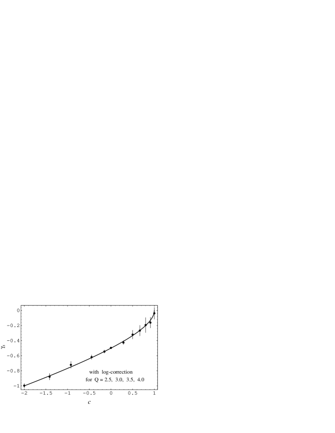
Figure 12: The measured string susceptibility $\gamma_{s}$ versus central charge $c$ and the theoretical curve. Logarithmic corrections are introduced in the fits for $Q=2.5,\,3.0,\,3.5$ and $4.0$.

The reason why the results for $c\approx 1$ disagree with the theoretical curve is possibly due to the fact that logarithmic corrections are not yet introduced. It is well known [12, 18] that logarithmic corrections play an important role in the vicinity of $c\approx 1$. Thus we assume that the partition function has the following asymptotic behavior for large $N$

$$Z(N)\sim e^{\lambda_{c}N}\,N^{\gamma_{s}-3}\,(\ln N)^{\alpha}\,,$$ (5.14)

where $\alpha$ is an additional parameter. The measured distributions $b_{N}(B)$ can now be fitted to the following parameterization:

$$\ln[b_{N}(B)] = a_{1}+(\gamma_{s}-2)\,\ln\biggl{[}B\,\biggl{(}1-\frac{B}{N}\biggr{)}\biggr{]}$$ (5.15)

$$\mbox{}+\alpha\,\ln[\ln B\cdot\ln(N-B)]+\frac{a_{2}}{B}\,,$$

for $Q=2.5,\,3.0,\,3.5$ and $4.0$. Then $\gamma_{s}$ with the logarithmic corrections versus central charge $c$ are plotted in fig.12.

The string susceptibility $\gamma_{s}$ with the logarithmic corrections for the various values of $Q$’s are in very good agreement with the theoretical curve. We can then conclude that the values of critical coupling $K_{c}(Q)$ evaluated numerically in the previous subsection are correct within errors.

5.3 The fractal dimension

The most straightforward definition of the fractal dimension is given by

$$N(r)=r^{d_{F}},$$ (5.16)

where we count the number of triangles $N(r)$ inside $r$ steps from a marked triangle. In fact the fractal structure of the two-dimensional quantum gravity was first confirmed in this way by Kawamoto, Kazakov, Saeki and Watabiki for $c=-2$ scalar fermion model[5]. In these analyses they needed 5 million triangles to obtain the reliable value of the fractal dimension. It was later recognized that finite size scaling hypothesis is very useful to evaluate the fractal dimension numerically and thus relatively small number of triangles is enough to obtain very accurate fractal dimension for $c=-2$ model[15],[16]. Here we use finite size scaling hypothesis to obtain the $c$-dependence of the fractal dimension.

It has already been recognized numerically in [5] that the total perimeter length $s_{N}(r)$ measured at geodesic distance $r$ from a marked triangle grows

$$s_{N}(r)=r^{d_{F}-1}.$$ (5.17)

This fact triggered the investigation of analytic derivation of transfer matrix for two dimensional random surface of quantum gravity for $c=0$ model[7]. It has then been recognized that two point function of random surface can be related to the measurement of $s_{N}(r)$ [9, 14, 43].

In the case of pure gravity ($c=0$) ”two-point function” with fixed volume $A$ is defined by

$$S_{A}(R)=\frac{1}{Z(A)}\,\int{\cal D}[g]\,\delta(\int d^{2}x\sqrt{g}-A)\,\frac{1}{A}\,\int\!d^{2}x\sqrt{g}\,\int\!d^{2}x^{\prime}\sqrt{g}\,\delta(D_{g}(x,x^{\prime})-R)\,,$$ (5.18)

where $D_{g}(x,x^{\prime})$ denotes the geodesic distance between the points labeled by $x$ and $x^{\prime}$ measured with respect to $g$. Then $S_{A}(R)\,dR$ is the average area of a spherical shell of thickness $dR$ and radius $R$ from a marked point on the manifold. We recognize that the lattice triangulation version of $S_{A}(R)$ corresponds to $s_{N}(r)$. According to the numerical result, we expect to have a relation

$$S_{A}(R)\sim R^{d_{F}-1}~{}~{}~{}~{}\mbox{for \ $R\sim 0$}\,.$$ (5.19)

In case of pure gravity ($c=0$) $S_{A}(R)$ was calculated analytically

$$S_{A}(R)=R^{3}f(R/A^{\frac{1}{4}})\,,$$ (5.20)

where $f(x)\sim e^{-x^{4/3}}$ for large $x$ [9, 14]. This analytic result is consistent with the calculation of the fractal dimension $d_{F}=4$ for $c=0$ model derived by transfer matrix formalism [7]. This result, however, strongly suggests the following scaling hypothesis for general matter central charge $c$ coupled two dimensional quantum gravity:

$$S_{A}(R)=A^{1-1/d_{F}}F(R/A^{1/d_{F}})\,,$$ (5.21)

where

$$F(x)\sim x^{d_{F}-1},~{}~{}~{}~{}x\ll 1\,.$$ (5.22)

This beautiful scaling behavior was observed with a high accuracy in the very systematic numerical analyses of the fractal structure of two-dimensional quantum gravity coupled to $c=-2$ matter[15, 16]. Here we assume that the scaling hypothesis works in general for the general matter central charge $-2\leq c\leq 1$.

Figure 13: The best linear fit to eq.(5.26) for $Q=2.5$ and $0.5$ as examples, by the decay of the peak of $s_{N}(r)/N$ with $N$.

Figure 14: The best linear fit to eq.(5.27) for $Q=2.5$ and $0.5$ as examples, by the decay of the inverse average radius $1/\langle r\rangle_{N}$ with $N$.

In our numerical simulations we define a geodesic distance as a “triangle distance” instead of link distance on a triangulation for saving the CPU time. The triangle distance denotes the shortest path along neighboring triangles between the two separate triangles. Therefore the triangle distance is equal to the “edge distance” in the dual $\varphi^{3}$-graph. Then the discretized analogue of $S_{A}(R)$, $s_{N}(r)$ with $A=Na^{2}(a^{2}=1)$, consists of all triangles with triangle distance $r$ measured from a marked triangle. Corresponding to the above continuum description we expect the following behavior for $s_{N}(r)$:

$$s_{N}(r)\sim N^{1-1/d_{F}}\,F(x)\,,~{}~{}~{}~{}~{}x=\frac{r}{N^{1/d_{F}}}\,,$$ (5.23)

and we expect $F(x)$ to behave as $x^{d_{F}-1}$ for small $x$.

In order to measure correlation function $s_{N}(r)$ the simulations were carried out with lattice sizes ranging; $N=100,\,200,\,400,\,800,\,1600,\,3200$ and $6400$ for $Q=0.0,\,0.05,\,0.2,\,0.5$ and $0.8$. For $Q=1.0,\,1.5,\,2.0,\,2.5,\,3.0,\,3.5$ and $4.0$ we have performed the simulations with lattice sizes ranging; $N=100\sim 6400$ and $12800$. For each lattice size ranging; $N=100\sim 1600$ the number of independent samples are $100K$, and we choose $20$ initial random vertices (rv) on each configuration. Then the number of independent samples is $50K\times 40({\rm rv})$ for $N=3200$, $20K\times 100({\rm rv})$ for $N=6400$ and $10K\times 200({\rm rv})$ for $N=12800$, respectively. The values of $Q$’s and its critical couplings $K_{c}(Q)$ are shown in table 2.

Figure 15: The measured fractal dimension $d_{F}$ by the decay of peak versus central charge $c$ and the three theoretical curves given by eqs. (2.12), (2.20) and (2.32).

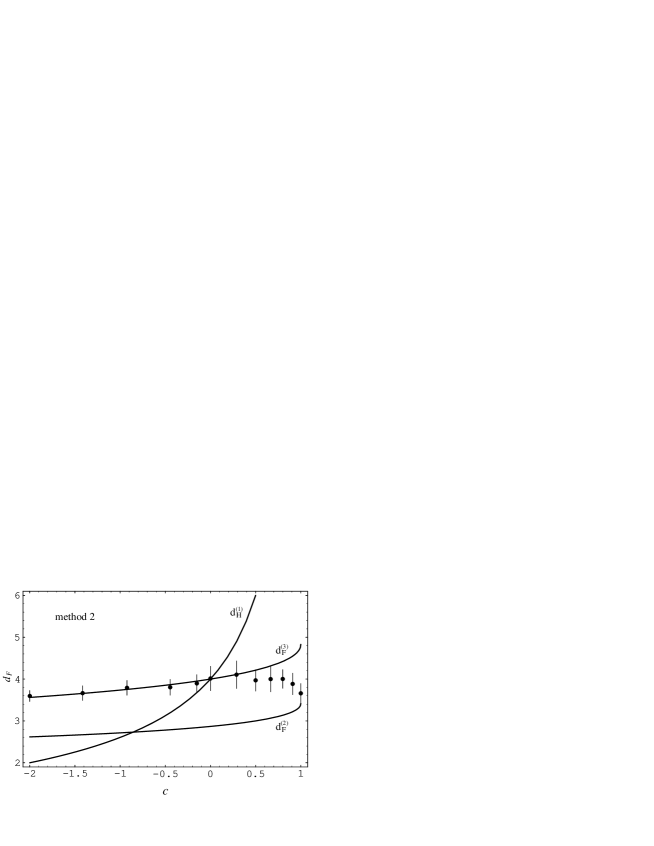
Figure 16: The measured fractal dimension $d_{F}$ by the average radius versus central charge $c$ and the three theoretical curves given by eqs. (2.12), (2.20) and (2.32).

In order to extract the fractal dimensions $d_{F}$ from the scaling relation (5.23), It is crucial to introduce the so-called shift parameter $a$ [14, 15, 16] which accommodate the finite size effects. This parameter $a$ is considered as the leading order correction in the scaling variable $x=r/N^{1/d_{F}}$. This is reasonable from the point of view that the shortest distances may include lattice artifacts, and thus we can not expect an exact agreement with the continuum formulae. On the other hand, in order to incorporate the higher order corrections in the scaling variable $x$ we need to introduce a second shift parameter $b$ [14]: $N^{1/d_{F}}\to N^{1/d_{F}}+b$. In this way we are led to a “phenomenological” scaling variable $x$

$$x=\frac{r+a}{N^{1/d_{F}}+b}\,.$$ (5.24)

In the present simulations with small lattice sizes (at most $N\sim 10^{3}$) we need to introduce the parameter $b$, however, it is numerically very hard to determine the optimal values of three parameters $a,\,b$ and $d_{F}$ in the case of the gravity coupled to matter. Although such optimal values of parameters are obtained, they keep the dependence on lattice size.

We have extracted the fractal dimensions $d_{F}$ by the following method. First we use the decay of the peak of $s_{N}(r)/N$ with $N$ (this is similar to the use of finite-size scaling in the case of the percolation susceptibility). From eq.(5.23) we expect the following scaling behavior:

$$s_{N}(r)/N\sim N^{-1/d_{F}}\,.$$ (5.25)

We have divided $N$’s into three successive divisions such as $N$’s ($(100,200,400),\\ (200,400,800),$ etc.), and we have performed to fit $s_{N}(r)/N=a_{1}\,N^{-1/d_{F}}$ for each successive divisions by two parameters. In this way the $d_{F}$ dependence on $N$ becomes clear. Then we further assume the following scaling behavior:

$$|1/d_{F}(N)-1/d_{F}(\infty)|\sim N^{-\alpha}\,,$$ (5.26)

where we can extrapolate $1/d_{F}(\infty)$ by a linear fit to eq.(5.26). This is shown in fig.13 for $Q=2.5$ and $0.5$ as examples, where the estimation of error is based on a non-linear fits to $s_{N}(r)/N$. The values of $d_{F}$’s obtained in this way for the various values of $Q$’s are plotted in fig.15. Three theoretical curves given by the formulae; (2.12), (2.20) and (2.32), are shown to be compared. It is clear that the formula (2.32) is closer to the numerical values of the fractal dimension.

Secondly, in order to make use of the whole information of $s_{N}(r)$ we have used the average radius $\langle r\rangle_{N}$ of universes with volume $N$

$$\langle r\rangle_{N}\equiv\frac{1}{N}\sum_{r=0}^{\infty}\,r\;s_{N}(r)\sim N^{1/d_{F}}\,.$$ (5.27)

We can then expect $1/\langle r\rangle_{N}\sim N^{-1/d_{F}}$, where $d_{F}$ can be determined in the same way as above. In fig.14 we show the corresponding linear fits to eq.(5.27). The values of $d_{F}$’s obtained in this way for the various values of $Q$’s are plotted in fig.16.

These two independent results are consistent with each other and support the theoretical prediction $d_{F}^{(3)}(c)$.

6 Conclusion and Discussions

In this article we have shown the results of numerical investigations of the fractal dimension of two-dimensional quantum gravity coupled to the matter central charge $c$ for $-2\leq c\leq 1$. The $c$-dependence of the matter central charge is introduced by reformulating $Q$-state Potts model into the model which can be identified as a generalization of percolation cluster model, weighted percolation cluster model, on the random lattice. In this formulation $Q$ can be generalized into non-integer value and thus continuous $c$-dependence is realized and then we have called this model simply as the generalized Potts model. Since the model has a percolation cluster feature, we have formulated a new Metropolis algorithm to generate clusters on dynamically triangulated surface.

The $c$-dependence of the critical coupling $K_{c}$ is not known theoretically. We have evaluated the $c$-dependence of $K_{c}$ by measuring percolation probability and percolation susceptibility with the help of scaling hypothesis. The $c$-dependence of the critical coupling has similar behaviour as those of flat lattice. It is then very natural to expect that there is a theoretical solution of theoretical coupling $K_{c}$ in two-dimensional quantum gravity coupled to matter central charge $c$. The order of the phase transition is assumed to be second or even higher order at the critical point and we have not observed any evidence against this assumption. The string susceptibility is measured by the baby universe technique and has excellent agreement with the theoretical curve. It is recognized that the next leading logarithmic correction is important to improve the agreement with the theoretical prediction in particular for the region near $c\approx 1$. Several parameters were needed to incorporate the finite size effects. The string susceptibility measurement is carried out as a cross check of the critical values of $K_{c}$ and the result was perfectly consistent with the independent measurement of the critical exponent in the above.

The $c$-dependence of the fractal dimension is measured based on the two-point function of quantum surface with the finite size scaling hypothesis. We needed two extra parameters to accommodate the finite size corrections to the scaling parameter. Measurements are carried out by two methods; the decay behaviour of the peak of two-point function and the average radius of universes. The results agree well each other. The $c$-dependence of the fractal dimension is excellent agreement with the following theoretical prediction except for the region $c\approx 1$:

$$d_{F}^{(3)}(c)\ =\ 2\times\frac{\sqrt{25-c}\,+\,\sqrt{49-c}}{\sqrt{25-c}\,+\,\sqrt{1-c}}.$$ (6.1)

We consider that the deviation of the agreement of the numerical values of the fractal dimensions near $c\approx 1$ from the theoretical values is possibly due to the fact that the size of the lattice is not large enough to observe the possible discrete jump from the fractal dimension $c<1$ of eq.(6.1) to the value of branched polymer phase $d_{F}=2,\gamma_{s}=1/2$[44, 45, 46].

It is interesting to measure the change of fractal dimension very accurately in this delicate region near $c\approx 1$. The theoretical curve of the $c$-dependence of the fractal dimension has infinite slope at $c=1$ and then turns into imaginary value. We conjecture that the fractal phase of two dimensional quantum gravity $c<1$ turns into branched polymer phase in $1<c$. We expect that there is a discrete jump of the fractal dimension at $c=1$. In order to measure this discrete jump numerically we may need huge number of triangles in the simulation.

It is interesting to compare with the measurement of the string susceptibility in three-dimensional simplicial gravity. In three dimensions tetrahedron is the fundamental simplex which corresponds to the triangle of two-dimensional quantum gravity. In three-dimensional dynamical triangulation the gravitational constant can be a free parameter and plays a role of central charge $c$ of two-dimensional quantum gravity. It was measured that the string susceptibility changes from negative region to the positive region where branched polymer phase is expected[47]. Here again the phase change from the fractal phase to the branched polymer phase is expected. For realistic higher dimensional simplicial quantum gravity it would be important to understand the phase change such as the fractal-branched polymer phase change.

$~{}~{}Q~{}~{}$	# triangles	range of $K$	interval of $K$	# samples
0.2	100	0.20 $\sim$ 0.58	0.02 $\times$ 20 (points)	20000
	200	0.30 $\sim$ 0.58	0.02 $\times$ 15 (points)	20000
	400	0.36 $\sim$ 0.64	0.02 $\times$ 15 (points)	20000
	800	0.40 $\sim$ 0.67	0.03 $\times$ 10 (points)	20000
	1600	0.48 $\sim$ 0.66	0.02 $\times$ 10 (points)	20000
	3200	0.47 $\sim$ 0.74	0.03 $\times$ 10 (points)	5000
0.4	100	0.42 $\sim$ 0.80	0.02 $\times$ 20 (points)	20000
	200	0.53 $\sim$ 0.81	0.02 $\times$ 15 (points)	20000
	400	0.61 $\sim$ 0.89	0.02 $\times$ 15 (points)	20000
	800	0.66 $\sim$ 0.93	0.03 $\times$ 10 (points)	20000
	1600	0.75 $\sim$ 0.93	0.02 $\times$ 10 (points)	20000
	3200	0.74 $\sim$ 1.01	0.03 $\times$ 10 (points)	5000
0.6	100	0.57 $\sim$ 1.01	0.02 $\times$ 23 (points)	20000
	200	0.71 $\sim$ 1.05	0.02 $\times$ 18 (points)	20000
	400	0.77 $\sim$ 1.09	0.02 $\times$ 17 (points)	20000
	800	0.83 $\sim$ 1.10	0.03 $\times$ 10 (points)	20000
	1600	0.86 $\sim$ 1.16	0.03 $\times$ 11 (points)	20000
	3200	0.86 $\sim$ 1.19	0.03 $\times$ 12 (points)	10000
0.8	100	0.70 $\sim$ 1.14	0.02 $\times$ 23 (points)	20000
	200	0.83 $\sim$ 1.11	0.02 $\times$ 15 (points)	20000
	400	0.91 $\sim$ 1.19	0.02 $\times$ 15 (points)	20000
	800	0.95 $\sim$ 1.22	0.03 $\times$ 10 (points)	20000
	1600	0.97 $\sim$ 1.27	0.03 $\times$ 11 (points)	20000
	3200	1.02 $\sim$ 1.29	0.03 $\times$ 10 (points)	10000

Table 3: The lattice sizes, ranges of the coupling constant $K$ and the number of samples in which we measure the finite-size percolation susceptibility $\chi_{N}(K)$ for $Q=0.2,\,0.4,\,0.6$ and $0.8$.

$~{}~{}Q~{}~{}$	# triangles	range of $K$	interval of $K$	# samples
1.0	100	0.82 $\sim$ 1.20	0.02 $\times$ 20 (points)	20000
	200	0.94 $\sim$ 1.22	0.02 $\times$ 15 (points)	20000
	400	1.00 $\sim$ 1.32	0.02 $\times$ 17 (points)	20000
	800	1.05 $\sim$ 1.32	0.03 $\times$ 10 (points)	20000
	1600	1.13 $\sim$ 1.31	0.02 $\times$ 10 (points)	20000
	3200	1.14 $\sim$ 1.34	0.02 $\times$ 11 (points)	10000
1.5	100	1.01 $\sim$ 1.39	0.02 $\times$ 20 (points)	20000
	200	1.13 $\sim$ 1.41	0.02 $\times$ 15 (points)	20000
	400	1.19 $\sim$ 1.47	0.02 $\times$ 15 (points)	20000
	800	1.28 $\sim$ 1.46	0.02 $\times$ 10 (points)	20000
	1600	1.31 $\sim$ 1.49	0.02 $\times$ 10 (points)	20000
	3200	1.33 $\sim$ 1.51	0.02 $\times$ 10 (points)	10000
2.0	100	1.10 $\sim$ 1.60	0.02 $\times$ 26 (points)	20000
	200	1.20 $\sim$ 1.60	0.02 $\times$ 21 (points)	20000
	400	1.28 $\sim$ 1.64	0.02 $\times$ 19 (points)	20000
	800	1.37 $\sim$ 1.61	0.02 $\times$ 13 (points)	20000
	1600	1.41 $\sim$ 1.63	0.02 $\times$ 12 (points)	20000
	3200	1.45 $\sim$ 1.63	0.02 $\times$ 10 (points)	10000
2.5	100	1.26 $\sim$ 1.64	0.02 $\times$ 20 (points)	20000
	200	1.37 $\sim$ 1.65	0.02 $\times$ 15 (points)	20000
	400	1.42 $\sim$ 1.70	0.02 $\times$ 15 (points)	20000
	800	1.50 $\sim$ 1.68	0.02 $\times$ 10 (points)	20000
	1600	1.53 $\sim$ 1.71	0.02 $\times$ 10 (points)	20000
	3200	1.54 $\sim$ 1.72	0.02 $\times$ 10 (points)	10000

Table 4: The same of table 3 for $Q=1.0,\,1.5,\,2.0$ and $2.5$.

$~{}~{}Q~{}~{}$	# triangles	range of $K$	interval of $K$	# samples
3.0	100	1.35 $\sim$ 1.73	0.02 $\times$ 20 (points)	20000
	200	1.46 $\sim$ 1.74	0.02 $\times$ 15 (points)	20000
	400	1.50 $\sim$ 1.78	0.02 $\times$ 15 (points)	20000
	800	1.59 $\sim$ 1.77	0.02 $\times$ 10 (points)	20000
	1600	1.60 $\sim$ 1.80	0.02 $\times$ 11 (points)	20000
	3200	1.62 $\sim$ 1.80	0.02 $\times$ 10 (points)	10000
3.5	100	1.40 $\sim$ 1.78	0.02 $\times$ 20 (points)	20000
	200	1.53 $\sim$ 1.81	0.02 $\times$ 15 (points)	20000
	400	1.58 $\sim$ 1.86	0.02 $\times$ 15 (points)	20000
	800	1.66 $\sim$ 1.84	0.02 $\times$ 10 (points)	20000
	1600	1.68 $\sim$ 1.86	0.02 $\times$ 10 (points)	20000
	3200	1.69 $\sim$ 1.87	0.02 $\times$ 10 (points)	10000
4.0	100	1.42 $\sim$ 1.90	0.02 $\times$ 25 (points)	20000
	200	1.56 $\sim$ 1.90	0.02 $\times$ 18 (points)	20000
	400	1.65 $\sim$ 1.93	0.02 $\times$ 15 (points)	20000
	800	1.73 $\sim$ 1.91	0.02 $\times$ 10 (points)	20000
	1600	1.74 $\sim$ 1.92	0.02 $\times$ 10 (points)	20000
	3200	1.75 $\sim$ 1.93	0.02 $\times$ 10 (points)	10000

Table 5: The same of table 3 for $Q=3.0,\,3.5$ and $4.0$.

Acknowledgments

We would like to thank I. Kostov and Y. Watabiki for useful discussions at the very early stage of this work. This work is supported in part by Japanese Ministry of Education, Science, Sports and Culture under the grant number 13640250.

References

- [1] V. Knizhnik, A.M. Polyakov and A. Zamolodchikov, Mod. Phys. Lett. A3 (1988) 819.
- [2] J. Distler, Z. Hlousek and H. Kawai, Mod. Phys. Lett. A5 (1990) 1093.
- [3] H. Kawai and M. Ninomiya, Nucl. Phys. B336 (1990) 115.
- [4] M. E. Agishtein and A. A. Migdal, Int. J. Mod. Phs. C1 (1990) 165; Nucl. Phys. B350 (1991) 690.
- [5] N. Kawamoto, V.A. Kazakov, Y. Saeki and Y. Watabiki, Phys. Rev. Lett. 68 (1992) 2113.
- [6] N. Kawamoto, Y. Saeki and Y. Watabiki, unpublished; Y. Watabiki, Progress in Theoretical Physics, Suppl. No. 114 (1993) 1; N. Kawamoto, in Proceedings of Nishinomiya-Yukawa workshop, Nishinomiya 1992, Quantum gravity, ed. K. Kikkawa and M. Ninomiya (World Scientific) p. 112; In First Asia-Pacific Winter School for Theoretical Physics 1993, Proceedings, Current Topics in Theoretical Physics, ed. Y.M. Cho (World Scientific).
- [7] H. Kawai, N. Kawamoto, T. Mogami and Y. Watabiki, Phys. Lett. B306 (1993) 19.
- [8] Y. Watabiki, Nucl. Phys. B441 (1995) 119; Phys. Lett. B346 (1995) 46.
- [9] J. Ambjørn and Y. Watabiki, Nucl. Phys. B445 (1995) 129.
- [10] J. Ambjørn, C.F. Kristjansen and Y. Watabiki, Nucl. Phys. B504 (1997) 555.
- [11] S. Oda, N. Tsuda and T. Yukawa, Prog. Theor. Phys. 99 (1998) 875.
- [12] S. Jain, and S.D. Mathur, Phys. Lett. B286 (1992) 239.
- [13] J. Ambjørn, S. Jain, and G. Thorleifsson, Phys. Lett. B307 (1993) 34.
- [14] J. Ambjørn, J. Jurkiewicz and Y. Watabiki, Nucl. Phys. B454 (1995) 313.
- [15] J. Ambjørn, K.N. Anagnostopoulos, T. Ichihara, L. Jensen, N. Kawamoto, Y. Watabiki and K. Yotsuji, Phys. Lett. B397 (1997) 177.
- [16] J. Ambjørn, K.N. Anagnostopoulos, T. Ichihara, L. Jensen, N. Kawamoto, Y. Watabiki and K. Yotsuji, Nucl. Phys. B511 (1998) 673.
- [17] J. Ambjørn and K.N. Anagnostopoulos, Nucl. Phys. B497 (1997) 445.
- [18] J. Ambjørn and G. Thorleifsson, Phys. Lett. B323 (1994) 7.
- [19] R.B. Potts, Proc. Camb. Phil. Soc. 48 (1952) 106.
- [20] C.M. Fortuin and P.W. Kasteleyn, J. Phys. Soc. Jpn. Suppl. 26 (1969) 11; Physica 57 (1972) 536.
- [21] J. Jurkiewicz, A. Krzywicki, B. Petersson and B. Soderberg, Phys. Lett. B213 (1988) 511; C.F. Baillie and D.A. Johnston, Phys. Lett. B286 (1992) 44; S. Catterall, J. Kogut and R. Renken, Phys. Lett. B292 (1992) 277; J. Ambjørn, B. Durhuus, T. Jonsson and G. Thorleifsson, Nucl. Phys. B398 (1993) 568; J. Ambjørn, G. Thorleifsson and M. Wexler, Nucl. Phys. B439 (1995) 187.
- [22] J. Ambjørn, G. Thorleifsson and M. Wexler, Nucl. Phys. B439 (1995) 187.
-
[23]
F. David,
Mod. Phys. Lett. A3 (1988) 651,
J. Distler and H. Kawai, Nucl. Phys. B321 (1989) 509. -
[24]
S. Weinberg, in General Relativity, an Einstein centenary
Survey, ed. S. W. Hawking and W. Israel (Cambridge University
Press, 1979) p. 790,
R. Gastmans, R. Kallosh and C. Truffin, Nucl. Phys. B133 (1978) 417,
S.M. Christensen adn M.J. Duff, Phys. Lett. B79 (1978) 213. - [25] E. Ising, Z. Physik 31 (1925) 253.
- [26] R.J. Baxter, S.B. Kelland and F.Y. Wu, J. Phys. A9 (1976) 397.
- [27] W.T. Tutte, J. Combinatorial Theory 2 (1967) 301.
- [28] F.Y. Wu, J. Phys. A10 (1977) L113.
- [29] J.N.V. Temperley and E.H. Lieb, Proc. R. Soc. London Ser. A322 (1971) 251.
- [30] Vl.S. Dotsenko, Nucl. Phys. B235 (1984) 54.
- [31] Vl.S. Dotsenko and V.A. Fateev, Nucl. Phys. B240 (1984) 312.
- [32] R.J. Glauber, J. Math. Phys. 4 (1963) 294.
- [33] M. Sweeny, Phys. Rev. B27 (1983) 4445.
- [34] V.A. Kazakov, I.K. Kostov and A.A. Migdal, Phys. Lett. B157 (1985) 295; D.V. Boulatov, V.A. Kazakov, I.K. Kostov and A.A. Migdal, Nucl. Phys. B275 (1986) 641.
- [35] V.A. Kazakov, Phys. Lett. A119 (1986) 140.
- [36] D.V. Boulatov and V.A. Kazakov, Phys. Lett. B186 (1987) 379.
- [37] D. Stauffer, Introduction to Percolation Theory, (Taylor & Francis, 1985).
- [38] M.E. Fisher and M.N. Barber, Phys. Rev. Lett. 28 (1972) 1516.
- [39] M.N. Barber and W. Selke, J. Phys. A15 (1982) L617.
- [40] T. Kihara, Y. Midzuno and T. Shizume, J. Phys. Soc. Japan 9 (1954) 681.
- [41] D. Kim and R. Joseph, J. Phys. C7 (1974) L167.
- [42] H. Kawai, Nucl. Phys. B26(Proc. Suppl.) (1992) 93.
- [43] J. Ambjørn, B. Durhuus and T. Jonsson, Quantum Geometry, (Cambridge University Press, 1997).
- [44] J. Ambjørn, B. Durhuus and T. Jonsson, Phys. Lett. B244 (1990) 403.
- [45] B. Durhuus, Nucl. Phys. B426 (1994) 203.
- [46] J. Jurkiewicz and A. Krzywicki, Phys. Lett. B392 (1997) 291.
- [47] J. Ambjørn, D.V. Boulatov, N. Kawamoto and Y. Watabiki, Phys. Lett. B480 (2000) 319.