The staggered domain wall fermion method

Abstract

A different lattice fermion method is introduced. Staggered domain wall fermions are defined in $2n+1$ dimensions and describe $2^{n}$ flavors of light lattice fermions with exact U(1)$\times$U(1) chiral symmetry in $2n$ dimensions. As the size of the extra dimension becomes large, $2^{n}$ chiral flavors with the same chiral charge are expected to be localized on each boundary and the full SU($2^{n}$)$\times$SU($2^{n}$) flavor chiral symmetry is expected to be recovered. SDWF give a different perspective into the inherent flavor mixing of lattice fermions and by design present an advantage for numerical simulations of lattice QCD thermodynamics. The chiral and topological index properties of the SDWF Dirac operator are investigated. And, there is a surprise ending…

I Introduction

Lattice fermions are elusive. They not only present enormous challenges to numerical simulations of lattice QCD and other strongly interacting field theories but also pose in a most blatant way the problem of non-perturbative regularization of chiral gauge theories. Obviously the two problems have a common source. In the past several years enormous progress has been made in this direction. Interestingly, extra dimensions have been used again in theoretical physics, except this time the dimension is a tool to generate the correct low energy physics.

Domain wall fermions were introduced in Kaplan (1992, 1993); Narayanan and Neuberger (1993a, 1994a); Frolov and Slavnov (1993, 1994). A large volume of work has followed since. The reader is referred to the annual reviews Kikukawa (2002); Edwards (2002); Vranas (2001); Golterman (2001); Neuberger (2000); Luscher (2000); Blum (1999); Shamir (1996); Creutz (1995); Narayanan and Neuberger (1994b) and references therein. The DWF lattice regulator begins by defining a massive Wilson fermion Wilson (1977) in $2n+1$ dimensions. If the boundary condition at the edges of the extra dimension is free then chiral surface states develop with the plus chirality fermion exponentially bound on one wall and the minus chirality fermion on the other wall Shamir (1993). The two chiralities have an overlap that breaks chiral symmetry. As the size $L_{s}$ of the extra dimension increases the overlap tends to zero exponentially fast. As $L_{s}\to\infty$ the theory has a single massless Dirac fermion in $2n$ dimensions. Obviously, this construction addresses both problems mentioned above.

Since the DWF construction starts with massive Wilson fermions, it is easy to see that for any finite $L_{s}$ there can be none of the exact chiral symmetries available in the naive lattice fermion formulation. In return for this shortcoming, flavor mixing between doubler states inherent in naive fermions are pushed up to the scale of the lattice cut-off, making them irrelevant. Early in the development of lattice field theories, the staggered approach to lattice fermions was devised to preserve some of the exact chiral symmetries of naive fermions. This meant there was still flavor mixing between the remaining doubler states Kogut and Susskind (1975); Banks et al. (1976); Susskind (1977). In the spirit of staggered fermions, our domain wall construction presented here will preserve some exact chiral symmetry at any $L_{s}$ at the cost of introducing flavor mixing between light fermion doublers. Flavor symmetry violations should be exponentially suppressed in the $L_{s}\to\infty$ limit. A preliminary version of this work was presented in Fleming and Vranas (2002).

Staggered domain wall fermions (SDWF) are similar to DWF in the use of exponential localization of surface states to counter unwanted features of lattice regularization. In our case, this means disentangling the inherent flavor mixing between light doubler states. As a result, even at finite $L_{s}$, they have an exact U(1)$\times$U(1) chiral symmetry very much like standard staggered fermions. This property makes them attractive for QCD thermodynamic simulations. As $L_{s}\to\infty$ the light surface states in the theory are expected to recover the full SU($2^{n}$)$\times$SU($2^{n}$) chiral symmetry. It must be noted that SDWF (and Wilson DWF as well) may not be able to develop light states if the coupling is extremely strong. Depending on one’s perspective, SDWF combine the nice properties of the domain wall method and staggered fermions. For simulations of QCD thermodynamics with standard DWF the reader is referred to Vranas (2000); Chen et al. (2001); Fleming (2001a, b).

We would like to draw the attention of the reader to a more subtle issue in this paper that might otherwise be overlooked. In most of what follows, the Saclay basis proposed by Kluberg-Stern et al. and predecessors Kluberg-Stern et al. (1983); Gliozzi (1982); van den Doel and Smit (1983) is used for its nice spin-flavor algebra. While this is formally equivalent to the standard bases used for numerical simulations Golterman and Smit (1984); Daniel and Sheard (1988), the transformation is gauge dependent and quite complicated. However, the conclusions we draw from our analytic work should be basis independent, The construction of actions suitable for numerical simulation will be discussed at the end of the paper.

One interesting result is that it may be possible to do numerical simulations directly in the Saclay basis when Pauli-Villars fields are introduced. This applies equally to staggered fermions as well as SDWF and may eliminate a serious obstacle for using the Saclay basis for simulation. The reason is that the gauge field dependent transformation that accompanies the basis change will cancel as part of the subtraction. We believe this is yet another example of the potential usefulness of doubly regularized lattice fermions Fleming (2001a).

For a semi-infinite extent in the extra dimension, the theory has four chiral fermions with the same chiral charges and is anomalous. To construct an anomaly free theory, we must use such “quadruplets” with charges as dictated by the corresponding anomaly cancellation condition. This is completely analogous to the case of Wilson DWF. Of course, in order to simulate a two flavor theory, a dynamical algorithm which effectively takes the square root of the fermionic determinant should be used. Further in the future, non-degenerate quark mass matrices could be explored to simulate the four lightest quarks.

The paper is organized as follows: The SDWF Dirac operator and action is defined in section II. The symmetries associated with the SDWF action are presented in section III. The flavor content is discussed in section IV and the free propagator is calculated in section V. The transfer matrix along the extra direction is given in section VI. The promised surprise is in section VII but the reader ought to work through the preceding sections first… The transcription to the single component basis, problems and future directions are presented in section VIII. A discussion about alternative actions is given in section IX. The paper is concluded with section X.

II Staggered Domain Wall Fermions

In this section the SDWF Dirac operator and action is presented in the Saclay basis Kluberg-Stern et al. (1983). Here, we show that in the free theory light fermion fields localize exponentially along the extra direction with suppressed flavor mixing.

The SDWF partition function is

$$Z=\int[dU]\int[d\overline{\Psi}d\Psi]\int[d\Phi^{\dagger}d\Phi]\ e^{-S}.$$ (1)

$U_{\mu}(x)$ is the gauge field, $x$ is a site coordinate vector in the $2n$ dimensional space and $\mu=1,2,\cdots,2n$. $\Psi(y,s)$ is the fermion field and $\Phi(y,s)$ is a bosonic Pauli-Villars (PV) field. $y$ is a hypercube coordinate vector related to the site vector $x$ by $x=2y+O+A$ where $O$ is a $2n$ dimensional binary vector indicating one of the $2^{2n}$ possible origins of the hypercubic structure and $A$ is a binary vector which indicates position within the given hypercube $y$. This implies the relations $y=(x-O-A)/2$ and $A=[(x-O)\bmod 2]$ between the vectors. $s=0,1,\cdots,L_{s}-1$ is a site coordinate in the $2n+1$ direction, where $L_{s}$ is the number of sites in this dimension.

The action $S$ is given by

$$S=S(\beta,L_{s},m_{0},m_{f};U,\overline{\Psi},\Psi,\Phi)=$$ (2)

$$S_{\text{G}}(\beta;U)+S_{\text{F}}(L_{s},m_{0},m_{f};\overline{\Psi},\Psi,V)+S_{\text{PV}}(L_{s},m_{0};\Phi^{\dagger},\Phi,V)$$

where

$$S_{\text{G}}=\beta\sum_{p}\left[1-\frac{1}{N_{c}}\text{Re\ Tr}U_{p}\right]$$ (3)

is the standard plaquette action with $\beta=2N_{c}/g_{0}^{2}$ with $g_{0}$ the lattice gauge coupling and $N_{c}$ the number of colors. The fermion action is

$$S_{\text{F}}=-\sum_{y,y^{\prime},s,s^{\prime}}\overline{\Psi}(y,s)D_{\text{F}}(y,s;y^{\prime},s^{\prime})\Psi(y^{\prime},s^{\prime})$$ (4)

with the fermion matrix given by

$$D_{\text{F}}(y,s;y^{\prime},s^{\prime})=\delta(s-s^{\prime})D(y,y^{\prime})+D^{\perp}(s,s^{\prime})\delta(y-y^{\prime})$$ (5)

where $D(y,y^{\prime})$ is the standard staggered action in the Saclay basis with the typical staggered mass (distance zero) set to zero and a different mass (distance one) proportional to $(1/a_{5}-m_{0})$ added as described below. Here are the expressions in a chiral basis in $2n=4$ dimensions. Extensions to other even dimensions are straightforward.

$$D=\left(\begin{array}[]{cc}B&C\\ -C^{\dagger}&-B\end{array}\right),$$ (6)

$$B=-\sum_{\mu}(\openone\otimes\xi_{5\mu})\left[\Delta_{\mu}(V)+\frac{m_{0}}{2}-\frac{1}{2a_{5}}\right],$$ (7)

$$C=-\frac{1}{4}\sum_{\mu}\sigma_{\mu}\nabla_{\mu}(V),$$ (8)

$$\Delta_{\mu}(V;y,y^{\prime})=\frac{1}{4}\left[\delta(y+\hat{\mu}-y^{\prime})V_{\mu}(y)+\delta(y-\hat{\mu}-y^{\prime})V^{\dagger}_{\mu}(y^{\prime})-2\delta(y-y^{\prime})\right],$$ (9)

$$\nabla_{\mu}(V;y,y^{\prime})=\frac{1}{4}\left[\delta(y+\hat{\mu}-y^{\prime})V_{\mu}(y)-\delta(y-\hat{\mu}-y^{\prime})V^{\dagger}_{\mu}(y^{\prime})\right]$$ (10)

where $\sigma_{1,2,3}$ are the Pauli matrices and $\sigma_{4}$ is the identity. $V_{\mu}(y)$ are the gauge links between hypercubes related to the $U_{\mu}(x)$ links of the gauge action by $V_{\mu}(y)=U_{\mu}(2y+O)\ U_{\mu}(2y+O+\hat{\mu})$. The parameter $m_{0}$ is the mass representing the “height” of the domain wall. The $s$-dependent part of the Dirac operator is exactly as for DWF but with a different mass mixing. Here we consider the action for $2^{n}$ degenerate flavors. For non-degenerate flavors the action is similar and can be constructed according to the rules outlined in section III.

$$D^{\perp}=D_{5}+H(m_{f}),$$ (11)

$$D_{5}(s,s^{\prime})=\left\{\begin{array}[]{ll}\frac{1}{a_{5}}\ P_{R}\delta(1-s^{\prime})&s=0\\ \frac{1}{a_{5}}[P_{R}\delta(s+1-s^{\prime})+P_{L}\delta(s-1-s^{\prime})]&0<s<L_{s}-1\\ \frac{1}{a_{5}}\ P_{L}\delta(L_{s}-2-s^{\prime})&s=L_{s}-1\end{array}\right.$$ (12)

The mass mixing term depends to whether $L_{s}$ is even or odd. For odd $L_{s}$ we have the following purely imaginary terms

$$H(m_{f};s,s^{\prime})=-\frac{1}{a_{5}}i\,m_{f}\left[P_{R}\delta(s-L_{s}+1)\delta(s^{\prime})+P_{L}\delta(s)\delta(L_{s}-1-s^{\prime})\right]$$ (13)

where $m_{f}$ is the degenerate mass of the flavor states localized on the domain wall. For even $L_{s}$ more care must be used in constructing the mass mixing term to preserve the exact U(1)$\times$U(1) symmetry (see section III). In that case the mass term does not just involve the boundary at $s=0$ and $L_{s}-1$ but also at $s=1$ and $L_{s}-2$. Furthermore notice that the terms are real. The different “reality” of the mass term for $L_{s}$ even/odd is just a reflection of a staggered wavefunction phase of the form $i^{(s-s^{\prime})}$. The even $L_{s}$ mass term is

$$H(m_{f};s,s^{\prime})=-\frac{m_{f}}{a_{5}} \left[P_{LR}\delta(s)\delta(L_{s}-2-s^{\prime})+P_{LL}\delta(s-1)\delta(L_{s}-1-s^{\prime})\right.$$

$$\left.+P_{RR}\delta(s-L_{s}+2)\delta(s^{\prime})+P_{RL}\delta(s-L_{s}-1)\delta(1-s^{\prime})\right].$$

The chiral and flavor projectors are

$$P_{R,L}=P_{\pm}=\frac{1\pm\gamma_{5}}{2},\quad F_{R,L}=F_{\pm}=\frac{1\pm\xi_{5}}{2},\quad P_{RL,RL}=P_{\pm\pm}=(P_{\pm}\otimes F_{\pm}).$$ (15)

The gamma matrices are taken in the standard chiral basis. For example $2n=4$ dimensions they are chosen to be

$$\gamma_{\mu}=\left(\begin{array}[]{cc}0&\sigma_{\mu}\\ \sigma_{\mu}^{\dagger}&0\end{array}\right),\mu=1,2,3\ \ \gamma_{4}=\left(\begin{array}[]{cc}0&1\\ 1&0\end{array}\right),\ \ \gamma_{5}=\left(\begin{array}[]{cc}1&0\\ 0&-1\end{array}\right)$$ (16)

with $\sigma_{\mu}$ the Pauli matrices. The flavor matrices are defined as usual Kluberg-Stern et al. (1983)

$$\xi_{\mu}=\gamma_{\mu}^{T}$$ (17)

and notations like $(\gamma_{5}\otimes\xi_{5\mu})$ mean $(\gamma_{5}\otimes\xi_{5}\xi_{\mu})$.

As with DWF, the PV action is designed to cancel the contribution of the heavy fermions. This is necessary because the number of heavy fermions is $\sim L_{s}$ and in the $L_{s}\rightarrow\infty$ limit they produce bulk type infinities Narayanan and Neuberger (1993a, 1994a, b); Narayanan and Neuberger (1995). There is some flexibility in the definition of the PV action since different actions could have the same $L_{s}\rightarrow\infty$ limit. However, the choice of the PV action may affect the approach to the $L_{s}\rightarrow\infty$ limit. Here the same approach as in Vranas (1997, 1998) was chosen. The $m_{f}=1$ case is exactly the quenched theory (infinitely massive fermions). The PV action is

$$S_{\text{PV}}=\sum_{x,x^{\prime},s,s^{\prime}}\Phi^{\dagger}(x,s)D_{\text{F}}[m_{f}=1](x,s;x^{\prime},s^{\prime})\Phi(x^{\prime},s^{\prime}).$$ (18)

The symmetries and detailed properties of the SDWF Dirac operator will be discussed in the rest of the paper. However, as a first check we verify that in the free case the SDWF Dirac operator indeed describes four flavors with the chiralities localized on the opposite walls. Following identical steps as in Kaplan (1992) we go to momentum space and demands that in order for light modes to exist there must be a wavefunction such that

$$D_{\text{F}}(k,s;k^{\prime},s^{\prime})\phi(k^{\prime},s^{\prime})=D_{\text{naive}}(k,s;k^{\prime},s^{\prime})\phi(k^{\prime},s^{\prime}).$$ (19)

In essence this equation demands that the extra term in the Dirac operator $D^{\perp}$ cancels the flavor breaking term $B$. From the above equations it is easy to see that Eq. (19) leads to

$$\sum_{s^{\prime}}\left\{\textstyle\frac{1}{a_{5}}\left[P_{+}\delta(s+1-s^{\prime})+P_{-}\delta(s-1-s^{\prime})\right]+{\textstyle\sum_{\mu}}(\gamma_{5}\otimes\xi_{5\mu})b_{\mu}\delta(s-s^{\prime})\right\}\phi(k,s^{\prime})=0$$ (20)

where

$$b_{\mu}=\frac{1-\cos{k_{\mu}}-m_{0}+1/a_{5}}{2}.$$ (21)

From this equation, it is easy to see that the $P_{\pm}$ projectors in the $s$-dependent part commute with the flavor breaking part so that each may be simultaneously diagonalized. This constraint alone effectively restricts the allowed projectors to the ones chosen here.

The solution is separable and $\phi(s)$ is the $s$-dependent part

$$\phi(s)=\left(\phi_{++},\phi_{+-},\phi_{-+},\phi_{--}\right)$$ (22)

where $\phi_{-+}(s)=P_{-+}\phi(s)$, etc. In this notation, we can write

$${\textstyle\sum_{\mu}}(\gamma_{5}\otimes\xi_{5\mu})b_{\mu}=\left(\begin{array}[]{rrrr}&\overline{b}&&\\ -\overline{b}^{\dagger}&&&\\ &&&-\overline{b}\\ &&\overline{b}^{\dagger}&\end{array}\right)$$ (23)

where

$${\overline{b}_{j}}=i\sigma_{j}^{*}b_{j},\quad j=1,2,3,\quad{\overline{b}_{4}}=b_{4}.$$ (24)

Solving Eqs. (20) relating nearest neighbor $s$ sites is a bit complicated because the flavor components mix and is not of interest for this discussion. On the other hand the solutions to these equations after iterating twice are simple. For $a_{5}=1$ we have

$$\begin{array}[]{rcl}\phi_{\pm+}(s\pm 2)&=&-\overline{b}\overline{b}^{\dagger}\phi_{\pm+}(s),\\ \phi_{\pm-}(s\pm 2)&=&-\overline{b}^{\dagger}\overline{b}\phi_{\pm-}(s).\end{array}$$ (25)

For free fermions, $[\overline{b},\overline{b}^{\dagger}]=0$ and $\overline{b}\overline{b}^{\dagger}$, $\overline{b}^{\dagger}\overline{b}$ are both proportional to the identity with eigenvalue

$$\lambda(\overline{b}\overline{b}^{\dagger})=\lambda(\overline{b}^{\dagger}\overline{b})=b^{2},$$ (26)

$$b=\sqrt{{\textstyle\sum_{\mu}}b_{\mu}^{2}}.$$ (27)

If we require that

$$b^{2}<1$$ (28)

then for a semi-infinite $s$ direction, $s$$\geq$0, only $\phi_{+\pm}$ is normalizable, while $\phi_{-\pm}$ is not. However, this is not enough to ensure that the doubler modes are not present. We must further require that the above condition excludes momenta with components larger or equal to $\pi$. This can be seen by writing out Eq. (28)

$$b^{2}=\frac{1}{4}\sum_{\mu}\left[(1-\cos{k_{\mu}})+(1-m_{0})\right]^{2}<1.$$ (29)

For momenta near the origins of the $n^{\text{th}}$ Brillouin zone (where $n$ is the number of momentum components near $\pi$) this gives

$$(1-m_{0})^{2}+n(1-m_{0})+n<1.$$ (30)

When $n=0$ the sufficient condition is

$$0<m_{0}<2,$$ (31)

same as for Wilson DWF. However, this condition does not ensure that the doubler modes are non-normalizable for all $n$. For example, for $n=1$ and $m_{0}=1.5$ both Eqs. (30) and (31) are satisfied making the $1^{\text{st}}$ Brillouin zone doubler wave functions normalizable. The range of $m_{0}$ needs to be further restricted. The following condition ensures that only the $0^{\text{th}}$ Brillouin zone wave function is normalizable

$$0<m_{0}<1.$$ (32)

The above is presented graphically in Fig. 1.

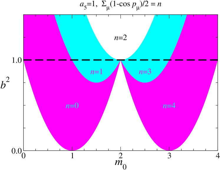
Figure 1: From Eq. (29): $b^{2}$ at the origins of the five Brillouin zones $n=[0,1,2,3,4]$ plotted vs. $m_{0}$.

It is straightforward to extend these results to the more general case of $0<a_{5}<1$.

III Symmetries

When constructing the SDWF action, it is important to preserve the symmetries of the massless staggered action Kogut and Susskind (1975); Jolicoeur et al. (1986). Of course, adding any new terms to the staggered action will break some of those symmetries, so we have to find new symmetries that involve the extra dimension. The symmetry transformations for the action in the Saclay basis of section II are presented below.

U(1)_e$\times$U(1)_o chiral rotations. The presence of this symmetry is one of the main motivations of this paper. The residual chiral symmetry of staggered fermions involves making separate chiral rotations on even and odd sites. Terms in $D^{\perp}$ are not invariant under these rotations unless we extend the notion of even and odd, including the extra dimension. The operator $\mathcal{S}$ is defined as

$$\mathcal{S}_{s,s^{\prime}}\equiv(-1)^{s}\delta(s-s^{\prime})$$ (33)

and then the extended even/odd projection operators are defined as

$$\overline{P}_{e} = {\textstyle\frac{1}{2}}\left[(\openone\otimes\openone)+\mathcal{S}(\gamma_{5}\otimes\xi_{5})\right],$$

$$\overline{P}_{o} = {\textstyle\frac{1}{2}}\left[(\openone\otimes\openone)-\mathcal{S}(\gamma_{5}\otimes\xi_{5})\right].$$ (34)

Using these projection operators the chiral transformation is

$$\Psi(y) \to \left(e^{i\theta_{e}}\overline{P}_{e}+e^{i\theta_{o}}\overline{P}_{o}\right)\ \Psi(y),$$

$$\overline{\Psi}(y) \to \overline{\Psi}(y)\ \left(e^{-i\theta_{o}}\overline{P}_{e}+e^{i\theta_{e}}\overline{P}_{o}\right).$$ (35)

Rotations by $\pi/2$. These rotations are in planes perpendicular to the extra dimension and the transformations are the same as the original staggered ones.

$\mu$-parity. These transformations reflect the $2n-1$ spacetime axes perpendicular to the spacetime axis in the $\hat{\mu}$ direction. $D^{\perp}$ is not invariant under this symmetry unless we also reflect the $s$ direction as well. If the reflection operator is defined as

$$\mathcal{R}_{s,s^{\prime}}\equiv\delta(L_{s}-1-s-s^{\prime})$$ (36)

then the transformation is

$$\begin{array}[]{rcl}\Psi(y,s)&\to&(\gamma_{\mu}\otimes\xi_{5})\mathcal{R}_{s,s^{\prime}}\ \Psi(y,s^{\prime}),\\ \overline{\Psi}(y,s)&\to&\overline{\Psi}(y,s^{\prime})\ \mathcal{R}_{s^{\prime},s}(\gamma_{\mu}\otimes\xi_{5}).\end{array}$$ (37)

Shift by one lattice spacing. The $m_{0}-1/a_{5}$ term in the SDWF action breaks this standard staggered fermion symmetry at the expense of absorbing the renormalization of the flavor breaking term. That these terms are additively renormalized in the interacting theory follows from the work of Mitra and Weisz Mitra and Weisz (1983). Nevertheless, interesting methods to alleviate the breaking of this symmetry are discussed in section VIII. This symmetry relates to interactions inside a hypercube which are essentially non-physical. We feel that the breaking of this symmetry is a small sacrifice, but the issue certainly can and should be debated.

The symmetry transformation for the case $m_{0}=1/a_{5}$ is given. Already for staggered fermions, the symmetry transformation is complicated in the Saclay basis due to the imposed hypercubic structure of the formulation. For SDWF, there is an added complication. Some parts of the transformation require a reflection in the $s$ direction

$$\Psi(y)\to{\textstyle\frac{1}{2}}\left[(\openone\otimes\xi_{\mu})-(\gamma_{\mu 5}\otimes\xi_{5})\mathcal{R}\right]\Psi(y)$$

$$+{\textstyle\frac{1}{2}}\left[(\openone\otimes\xi_{\mu})+(\gamma_{\mu 5}\otimes\xi_{5})\mathcal{R}\right]\Psi(y+\hat{\mu}),$$

$$\overline{\Psi}(y)\to\overline{\Psi}(y){\textstyle\frac{1}{2}}\left[(\openone\otimes\xi_{\mu})-\mathcal{R}(\gamma_{5\mu}\otimes\xi_{5})\right]$$ (38)

$$+\overline{\Psi}(y+\hat{\mu}){\textstyle\frac{1}{2}}\left[(\openone\otimes\xi_{\mu})+\mathcal{R}(\gamma_{5\mu}\otimes\xi_{5})\right]$$

where $s$ indices have been suppressed.

IV Flavors of SDWF

In this section the SDWF flavor identification is made in the Saclay basis. From section II we see that for a finite extra direction with $L_{s}$ sites the $P_{+}$ components of all flavors are localized around $s$=0 while the $P_{-}$ components are localized around $s$=$L_{s}$$-$1. However, as already mentioned in section III one of the main goals of this paper is to preserve most of the staggered symmetries and particularly the U(1)_e$\times$U(1)_o chiral symmetry. For example, to generate the four-dimensional flavor components $q$ with $P_{++}$, we should choose $s$ near zero. If $s$=0 is chosen, $P_{++}q(y)=P_{++}\Psi(y,0)$, then these components also belong to the $P_{e}$ part of the fermion field. Therefore, to project flavor components with $P_{-+}$ we are not only restricted to choose $s$ near $L_{s}$$-$1 but also choose $s$ so these components belong to the $P_{o}$ part of the fermion field. Then, components $P_{\pm+}q$ will not mix even for finite $L_{s}$ because of the even/odd symmetry. In this example, we would like to pick $P_{-+}q(y)=P_{-+}\Psi(y,s)$ with $s$ being even and near $L_{s}$$-$1. So, if $L_{s}$ is odd then $s$=$L_{s}$$-$1 is a good choice. However, if $L_{s}$ is even, then we should choose $s$=$L_{s}$$-$2 instead.

$$\textstyle\begin{array}[]{c}\left[\begin{array}[]{c}\left(\begin{array}[]{c}\text{X}\\ x\\ x\\ x\end{array}\right)\\ \\ \left(\begin{array}[]{c}x\\ \text{X}\\ x\\ x\end{array}\right)\\ \\ \vdots\\ \\ \left(\begin{array}[]{c}x\\ x\\ \text{X}\\ x\end{array}\right)\\ \\ \left(\begin{array}[]{c}x\\ x\\ x\\ \text{X}\end{array}\right)\end{array}\right]\\ \\ \Psi\end{array}\!\!\!\!=\!\!\!\!\begin{array}[]{c}\left[\begin{array}[]{c}\left(\begin{array}[]{c}\text{X}\\ 0\\ 0\\ x\end{array}\right)\\ \\ \left(\begin{array}[]{c}0\\ \text{X}\\ x\\ 0\end{array}\right)\\ \\ \vdots\\ \\ \left(\begin{array}[]{c}x\\ 0\\ 0\\ x\end{array}\right)\\ \\ \left(\begin{array}[]{c}0\\ x\\ x\\ 0\end{array}\right)\end{array}\right]\\ \\ P_{e}\Psi\end{array}\!\!\!\!+\!\!\!\!\begin{array}[]{c}\left[\begin{array}[]{c}\left(\begin{array}[]{c}0\\ x\\ x\\ 0\end{array}\right)\\ \\ \left(\begin{array}[]{c}x\\ 0\\ 0\\ x\end{array}\right)\\ \\ \vdots\\ \\ \left(\begin{array}[]{c}0\\ x\\ \text{X}\\ 0\end{array}\right)\\ \\ \left(\begin{array}[]{c}x\\ 0\\ 0\\ \text{X}\end{array}\right)\end{array}\right].\\ \\ P_{o}\Psi\end{array}$$ (39)

Using the block notation of Eq. (22), an example for even $L_{s}$ is sketched in Eq. (39). In this equation $\Psi$($s$=0) is at the top and $\Psi$($s$=$L_{s}$$-$1) is at the bottom. The capital letters denote one of the correct choices. On the other hand if $L_{s}$ is odd, e.g. $L_{s}$=3, then

$$\begin{array}[]{c}\left[\begin{array}[]{c}\left(\begin{array}[]{c}\text{X}\\ \text{X}\\ x\\ x\end{array}\right)\\ \\ \left(\begin{array}[]{c}x\\ x\\ x\\ x\end{array}\right)\\ \\ \left(\begin{array}[]{c}x\\ x\\ \text{X}\\ \text{X}\end{array}\right)\end{array}\right]\\ \\ \Psi\end{array}\!\!\!\!=\!\!\!\!\begin{array}[]{c}\left[\begin{array}[]{c}\left(\begin{array}[]{c}\text{X}\\ 0\\ 0\\ x\end{array}\right)\\ \\ \left(\begin{array}[]{c}0\\ x\\ x\\ 0\end{array}\right)\\ \\ \left(\begin{array}[]{c}x\\ 0\\ 0\\ \text{X}\end{array}\right)\end{array}\right]\\ \\ P_{e}\Psi\end{array}\!\!\!\!+\!\!\!\!\begin{array}[]{c}\left[\begin{array}[]{c}\left(\begin{array}[]{c}0\\ \text{X}\\ x\\ 0\end{array}\right)\\ \\ \left(\begin{array}[]{c}x\\ 0\\ 0\\ x\end{array}\right)\\ \\ \left(\begin{array}[]{c}0\\ x\\ \text{X}\\ 0\end{array}\right)\end{array}\right].\\ \\ P_{o}\Psi\end{array}$$ (40)

We note that other choices for selecting flavor components near the boundaries are certainly possible.

V The SDWF propagator

The propagator in the Saclay basis in momentum space and for $m_{f}=0$ has the form

$$D^{-1}(s,s^{\prime})=G_{1}\ \epsilon(s-s^{\prime})+G_{3}\ \epsilon(s-s^{\prime}-1).$$ (41)

For $m_{f}\neq 0$ and $L_{s}=\text{multiple of 4}$ has the form

$$D^{-1}(s,s^{\prime})=\left[G_{1}+m_{f}G_{2}\right]\ \epsilon(s-s^{\prime})+G_{3}\ \epsilon(s-s^{\prime}-1).$$ (42)

For $L_{s}=\text{even but not multiple of 4}$, the propagator has the same form as in Eq. (42) but with $m_{f}\to-m_{f}$. For $L_{s}=\text{odd}$ the $m_{f}$ term is more complicated and is not given here. Nevertheless, based on sections II and III one can see that the form is similar.

$G_{1}(p;s,s^{\prime})$, $G_{2}(p;s,s^{\prime})$ and $G_{3}(p;s,s^{\prime})$ ($p$ is the momentum) are proportional to the identity in their flavor indices. Also, $G_{1}$ anti-commutes with $(\gamma_{5}\otimes\openone)$ while $G_{2}$ and $G_{3}$ commute with $(\gamma_{5}\otimes\openone)$. The flavor mixing is in the function $\epsilon(s)$

$$\begin{array}[]{rcll}\displaystyle\epsilon(s)&=&(\openone\otimes\openone),&(s\ \text{even})\\ \epsilon(s)&=&\frac{\textstyle\sum_{\mu}(\openone\otimes\xi_{5\mu})b_{\mu}}{\textstyle b},&(s\ \text{odd})\end{array}$$ (43)

where $|b|$ is given in Eq. (27). For $s-s^{\prime}$ even and $m_{f}$=0 the propagator has no flavor mixing except for the $G_{3}$ term in Eq. (41). In this term $\epsilon(\text{odd})$ breaks flavor in exactly the same way as for free staggered fermions. An exact U(1)$\times$U(1) symmetry is maintained. The matrix coefficient $G_{3}$ vanishes exponentially fast with $L_{s}$ for $s$, $s^{\prime}$ near opposing boundaries and therefore as $L_{s}\to\infty$ with $m_{f}$=0 the propagator anti-commutes with $(\gamma_{5}\otimes\openone)$ and has no flavor mixing provided $s-s^{\prime}$ is even. This is in accordance with the discussion in section IV. For $s-s^{\prime}$ odd more severe flavor mixing is present.

The $G_{1}$, $G_{2}$ and $G_{3}$ terms are

$$G_{1}(p:s,s^{\prime})=i^{(s-s^{\prime}-1)}\frac{1}{2}\sum_{\mu}\gamma_{\mu}\sin{p_{\mu}}\ \left[P_{+}G(s,s^{\prime})+P_{-}G(L_{s}-1-s,L_{s}-1-s^{\prime})\right],$$ (44)

$$G_{2}=-i^{(s-s^{\prime}-1)}\ \ \left[P_{+}\delta(s,0)G(L_{s}-1,s^{\prime})-\delta(s,L_{s}-1)P_{-}G(L_{s}-1,L_{s}-1-s^{\prime})\right],$$ (45)

$$G_{3} = i^{(s-s^{\prime}-1)}P_{+}\left[bG(s,s^{\prime})+i\theta_{+}(s)G(s-1,s^{\prime})\right]$$

$$+ P_{-}\left[bG(L_{s}-1-s,L_{s}-1-s^{\prime})+i\theta_{-}(s)G(L_{s}-2-s,L_{s}-1-s^{\prime})\right].$$

where

$$\begin{array}[]{rcll}\displaystyle\theta_{+}(s)&=&1,&(s\neq 0)\\ \theta_{+}(s)&=&0,&(s=0)\\ \theta_{-}(s)&=&1,&(s\neq L_{s}-1)\\ \theta_{-}(s)&=&0,&(s=L_{s}-1).\end{array}$$ (47)

There is an exact correspondence with the terms of the standard DWF propagator. In the notation of Vranas (1997, 1998) the symbol correspondences between SDWF and DWF are

$$G(p:s,s^{\prime})\to G_{+}(p:s,s^{\prime}),\ \ \ b\to b,\ \ \ \overline{p}\to\frac{1}{4}\overline{p}.$$ (48)

The reader is referred there for the detailed forms.

As can be seen the decay coefficient is now in terms of $b$ given in Eq. (27) instead of the DWF $b=\sum_{\mu}[1-\cos{p_{\mu}}]+1/a_{5}-m_{0}$. The localization condition for $m_{0}$ is over half the DWF range (see Eq. (31)). Also, for $L_{s}$ odd, the effective mass $m_{\text{eff}}$ has the same general form as in Wilson DWF Vranas (1997, 1998)

$$m_{\text{eff}}=(1-\frac{2n}{4}m_{0}^{2})(m_{f}+|1-m_{0}|^{L_{s}}).$$ (49)

VI The SDWF transfer matrix

The SDWF transfer matrix in the Saclay basis is presented. We can use the technique of Neuberger Neuberger (1998) to rewrite the free SDWF determinant in a form that allows for a quick identification of the transfer matrix. A complete Hamiltonian analysis is beyond the scope of this work.

After interchanging various rows and columns of the SDWF matrix, the determinant is equivalent to the determinant of the matrix

$$\left(\begin{array}[]{cccc}\alpha_{0}&&&\beta_{0}\\ \beta_{1}&\ddots&&\\ &\ddots&\alpha_{L_{s}-2}&\\ &&\beta_{L_{s}-1}&\alpha_{L_{s}-1}\end{array}\right)$$ (50)

where all of the $\alpha_{s}$ and $\beta_{s}$ are the block triangular matrices

$$\alpha_{s}=\left(\begin{array}[]{cc}-B&0\\ C&1/a_{5}\end{array}\right),\quad\beta_{s}=\left(\begin{array}[]{cc}1/a_{5}&-C^{\dagger}\\ 0&B\end{array}\right).$$ (51)

For $\alpha_{L_{s}-1}$ and $\beta_{0}$, $1/a_{5}$ is replaced with $-\mu/a_{5}$ so $\mu$ is a parameter that controls the boundary conditions: $\mu=\pm 1$ for (anti)periodic and $\mu=0$ for free. This parameter is used only for the derivation of the transfer matrix and it is not needed in the theory. In particular, the reader is cautioned against using $\mu$ as a mass parameter since it is inconsistent with the rules of section IV. The definitions of $B,C$ are given in Eqs. (7) and (8).

In this notation, following Neuberger’s construction leads to the SDWF determinant

$$D_{\text{F}}=(\text{fixed\ sign})(\det{B/a_{5}})^{L_{s}}\det{\left[\left(\begin{array}[]{cc}-\mu&0\\ 0&1\end{array}\right)-T^{-L_{s}}\left(\begin{array}[]{cc}1&0\\ 0&-\mu\end{array}\right)\right]}$$ (52)

and the SDWF transfer matrix identification

$$T=-\left(\begin{array}[]{cc}B^{-1}/a_{5}&B^{-1}C\\ C^{\dagger}B^{-1}&a_{5}[C^{\dagger}B^{-1}C-B]\end{array}\right).$$ (53)

We can easily check that

$$[C,(\openone\otimes\xi_{5})]=0,\quad\{B,(\openone\otimes\xi_{5})\}=0$$ (54)

and as a result

$$\{T,(\openone\otimes\xi_{5})\}=0.$$ (55)

Also since $B^{\dagger}=-B$ we can see that $T$ is also anti-Hermitian

$$T^{\dagger}=-T.$$ (56)

This is different from Wilson DWF and gives some idea why solving the zero mode problem in Eq. (25) simplifies when solving for the field two sites away. Obviously, standard transfer matrix manipulations should be done with the Hermitian transfer matrix $T^{2}$ which corresponds to a Hermitian Hamiltonian $H$.

VII About that surprise…

At this point the reader must be wondering: “What is the spectrum of the transfer matrix?” and “What is the corresponding Hamiltonian?” Here is where we were a bit surprised. Just in case the reader will later (after reading this section) be tempted to claim that there is no surprise, she/he is invited to guess the $a_{5}\to\infty$ limit Hamiltonian as well as the general $a_{5}$ spectrum of $T^{2}$.

We find, after some algebra, the following Hamiltonian $H_{0}$ corresponding to the $a_{5}\to 0$ limit of the transfer matrix

$$\lim_{a_{5}\to 0}-T^{2}=e^{-2a_{5}H_{0}},\quad H_{0}=-(\gamma_{5}\otimes\openone)\left(\begin{array}[]{cc}\frac{1}{2}\sum_{\mu}\Delta_{\mu}+m_{0}&C\\ -C^{\dagger}&\frac{1}{2}\sum_{\mu}\Delta_{\mu}+m_{0}\end{array}\right).$$ (57)

The first surprise is that $H_{0}$ is exactly diagonal in flavor. It is almost, but not exactly, the same as the standard overlap Hamiltonian $H_{w}$, as $\Delta_{\mu}$ has a factor of $\frac{1}{2}$ compared to $C$. Nevertheless, because $H_{0}$ is diagonal in flavor, the standard machinery of DWF can be directly applied.

For example, let us consider the spectrum of $H_{0}$. Following methods identical to Narayanan and Neuberger (1993a, 1994a, b); Narayanan and Neuberger (1995) we find that

$$H_{0}\left(\begin{array}[]{c}u\\ v\end{array}\right)=0\quad\Rightarrow\quad u^{\dagger}\Delta u+v^{\dagger}\Delta v-2m_{0}=0.$$ (58)

Because the matrices $\delta(y+\hat{\mu}-y^{\prime})V_{\mu}(y)$ are unitary the range for which this equation can have a solution (for all Brillouin zones) is

$$0<m_{0}<2\quad(a_{5}\to 0).$$ (59)

For $m_{0}$ in the above range $H_{0}$ can have zero eigenvalues that via the overlap formalism correspond to a change of index and to exact and robust zeros of the fermionic determinant. This can also be seen graphically in Fig. 2. The background field configuration is a smooth gauge field that has non-trivial topology Narayanan and Neuberger (1993b); Narayanan and Neuberger (1995). The plaquette value for that configuration (i.e. the sum in Eq. (3)) is about $0.05$. For the rest of the paper we will refer to this configuration as the “instanton” configuration.

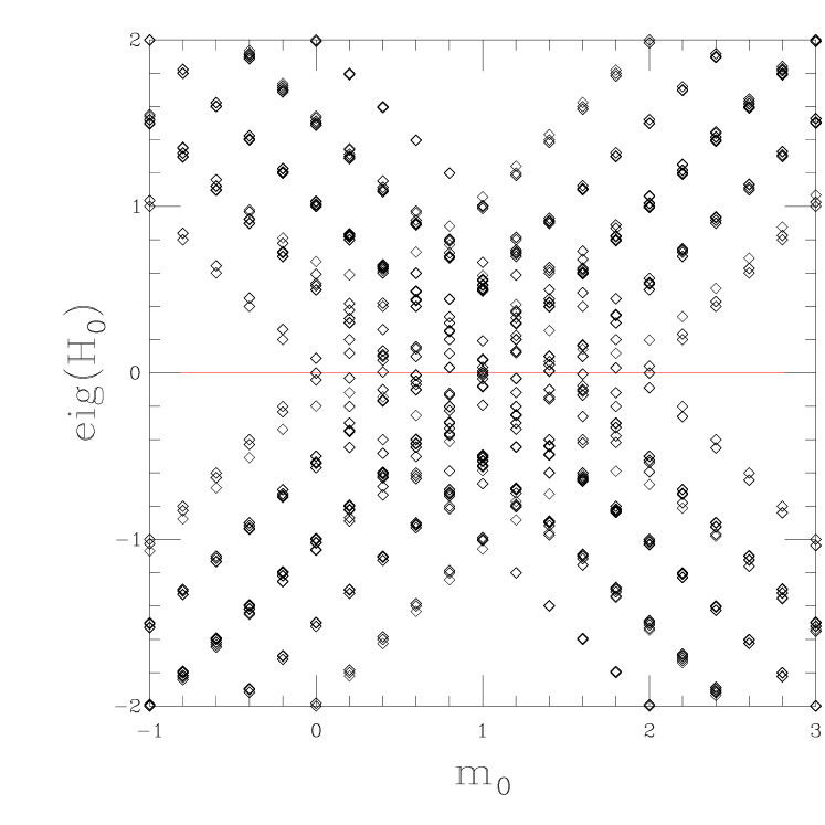
Figure 2: The spectrum of $H_{0}$ vs. $m_{0}$ for an SU(3) “instanton” background on a $2^{4}$ lattice of hypercubes.

The crossing diagrams were done for fermions in the Saclay basis with gauge fields $V_{\mu}(y)$ defined on a $2^{4}$ lattice of hypercubes. Since no attempt is made here to make a connection with the topological charge of the underlying gauge configurations $U_{\mu}(x)$, the reader can regard the gauge fields as examples “pulled out of a hat.” All numerical analysis was done by full diagonalization of the relevant matrices using the LAPACK libraries and an IBM-T20 Think Pad (which by the way performed brilliantly).

However, numerical simulations are done at non-zero $a_{5}$, typically at $a_{5}=1$. In standard DWF there is an exact connection between zero eigenvalues of $H_{0}$ and unit eigenvalues of the transfer matrix at any $a_{5}$. This correspondence does not hold here. As a result the analysis is more complicated. In other words

$$|\text{eig}(-T^{2})|=1\quad\not\Rightarrow\quad\text{eig}(H_{0})=0,\quad a_{5}\neq 0.$$ (60)

From Eqs. (55) and (56) we deduce that the spectrum of $-T^{2}$ is strictly real, positive and doubly degenerate because $T$ is anti-Hermitian and anticommutes with $(\openone\otimes\xi_{5})$. In $2n=2$ dimensions that would be the end of the story because there are only $2^{n}=2$ flavors. Two exact zero modes are produced for every crossing in the Hamiltonian spectrum. In $2n=4$ dimensions there are $2^{n}=4$ flavors and we do not have an exact correspondence between the degeneracy of the unit magnitude eigenvalues of $T$ and the number of flavors. This is problematic since this is a basic and defining property for a chiral theory.

For the “instanton” background the eigenvalue crossing diagram of

$$\lambda_{tm}=\log[\text{spectrum}\ (-T^{2})]$$ (61)

vs. $m_{0}$ is given in Fig. 3 for $a_{5}=1$. A closeup of the region around $m_{0}$=0 is shown and the eigenvalues are marked depending on the sign of the $\overline{q}(\gamma_{5}\otimes\openone)q$ where $q$ is the corresponding eigenvector. All eigenvalues in Fig. 3 are four-fold degenerate! The symbols for each eigenvalue are there but are literally overlapping. An example is given in Table 1. Also, the reader should observe that in Fig. 3 the transfer matrix eigenvector chirality does follow each flow line. This ensures that the four modes are of the same chirality and therefore a crossing should correspond to a net change of four in the index. It is of fundamental importance that this occurs here as it reassures us that on a given boundary of the extra dimension there are four flavors of light chiral fermions with the same chiral charge.

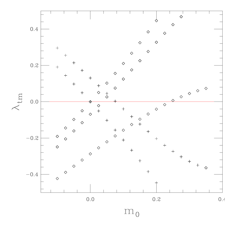
Figure 3: $\lambda_{tm}$ vs. $m_{0}$ for $a_{5}=1$ and an SU(3) “instanton” background (plaquette $\approx 0.05$) on a $2^{4}$ lattice of hypercubes. The diamonds represent eigenvectors of $T^{2}$ with chirality $+1$ while the pluses with $-1$. All eigenvalues are four-fold degenerate and are indistinguishable by the graphics. For an example please refer to Table 1.

Table 1: The near zero spectrum of $\log(-T^{2})$ for $m_{0}=0.2$ for an SU(3) “instanton” background on a $2^{4}$ lattice of hypercubes.

$m_{0}$	$\log{\lambda(-T^{2})}$
0.2	-0.0408683
0.2	-0.0408683
0.2	-0.0408683
0.2	-0.0408683
0.2	0.327367
0.2	0.327367
0.2	0.327367
0.2	0.327367

For a very rough background gauge field (plaquette $\approx 0.85$) the crossing diagram is given in Fig. 4. The eigenvalues are doubly degenerate and very nearly but not quite four-fold degenerate. The non degeneracy is small and almost non visible. One of the worst cases is presented in Table 2. The lack of exact four-fold degeneracy should be the subject of further research but it is obviously small even on this extreme background gauge field that is unlikely to occur in current numerical simulations of QCD. Furthermore, it would be interesting to study the transfer matrix in $2n\geq 6$ dimensions, where the required near-degeneracy should be $2^{n}$, to see if the same behavior persists.

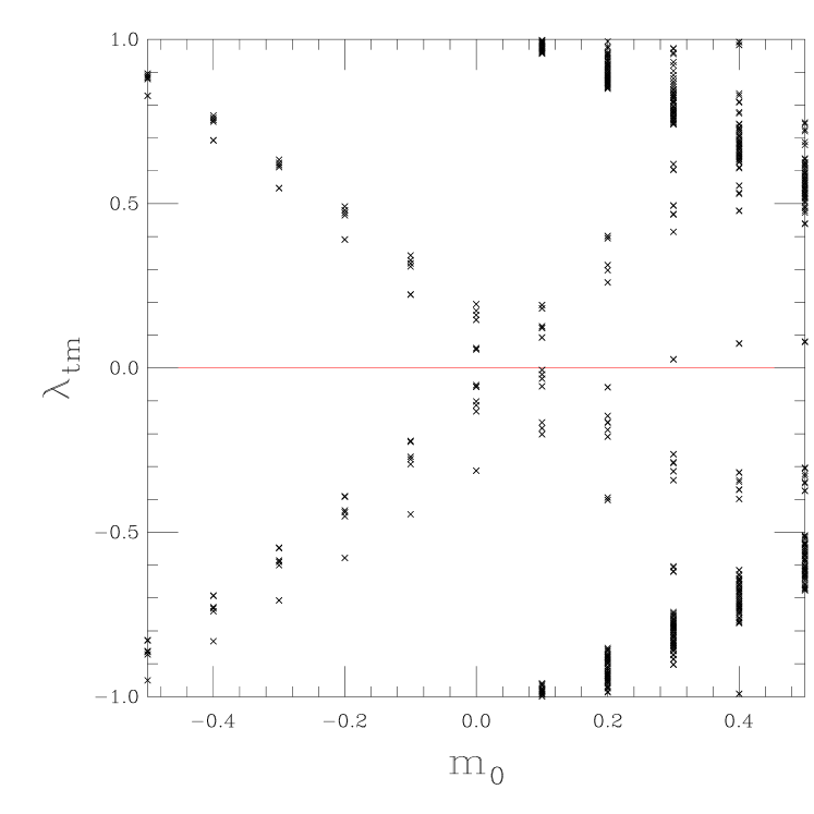
Figure 4: $\lambda_{tm}$ vs. $m_{0}$ for $a_{5}=1$ and a “rough” SU(3) background (plaquette $\approx 0.85$) on a $2^{4}$ lattice of hypercubes. All eigenvalues are two-fold degenerate and are indistinguishable by the graphics. Although there is no exact four-fold degeneracy the graphics can hardly distinguish the non-degeneracy. Please refer to Table 2.

Table 2: The near zero spectrum of $\log(-T^{2})$ for $m_{0}=0.3$ for a “rough” SU(3) background (plaquette $\approx 0.85$) on a $2^{4}$ lattice of hypercubes.

$m_{0}$	$log{\lambda(-T^{2})}$
0.3	-0.290045
0.3	-0.290045
0.3	-0.286291
0.3	-0.286291
0.3	-0.262638
0.3	-0.262638
0.3	-0.261551
0.3	-0.261551
0.3	0.0260566
0.3	0.0260566
0.3	0.0272779
0.3	0.0272779
0.3	0.414225
0.3	0.414225
0.3	0.414597
0.3	0.414597

Even with the lack of exact four-fold degeneracy, if we choose $m_{0}$ away from the crossing region then the fermion determinant will still have four exact zeros. This will only break down if $m_{0}$ is chosen between the two nearly degenerate sets of crossings. Of course, based on DWF studies at lattice spacings used in today’s simulations one expects dense crossings in the usable range of $m_{0}$. Then there will be configurations for which $m_{0}$ is between double-crossings that have split. As far as topology is concerned this will break flavor to some degree. Nevertheless, since in DWF the dense crossings correspond to small instantons and are unphysical we would expect that as the lattice spacing becomes smaller such configurations will become less important.

Nevertheless it is instructive to further study the spectrum of $T$ for unit magnitude eigenvalue. Because $T$ contains the inverse of $B$ it is hard to study analytically. However, in the subspace $|\lambda_{tm}|=1$ we can proceed as in Narayanan and Neuberger (1993a, 1994a, b); Narayanan and Neuberger (1995). In particular we find that

$$T\left(\begin{array}[]{c}u\\ v\end{array}\right)=\pm\ i\ T\left(\begin{array}[]{c}u\\ v\end{array}\right)\quad\Rightarrow\quad H_{p}\left(\begin{array}[]{c}u\\ v\end{array}\right)=0$$ (62)

where

$$H_{p}=\left(\begin{array}[]{cc}1+a_{5}iB&a_{5}C\\ a_{5}C^{\dagger}&-1-a_{5}iB\end{array}\right).$$ (63)

So, we can study the crossings of the spectrum of this pseudo-Hamiltonian $H_{p}$. The crossing range can be determined as before by using the unitarity of the matrices $\delta(y+\hat{\mu}-y^{\prime})V_{\mu}(y)$. There are two crossing ranges

$$0<m_{0}<2\quad\text{and}\quad\frac{2}{a_{5}}<m_{0}<\frac{2}{a_{5}}+2.$$ (64)

For the “instanton” background the crossing diagrams (for all Brillouin zones) are shown for $a_{5}=1$ in Fig. 5, $a_{5}=0.5$ in Fig. 6 and $a_{5}=0.25$ in Fig. 7 and the reader can see the agreement with Eq. (64).

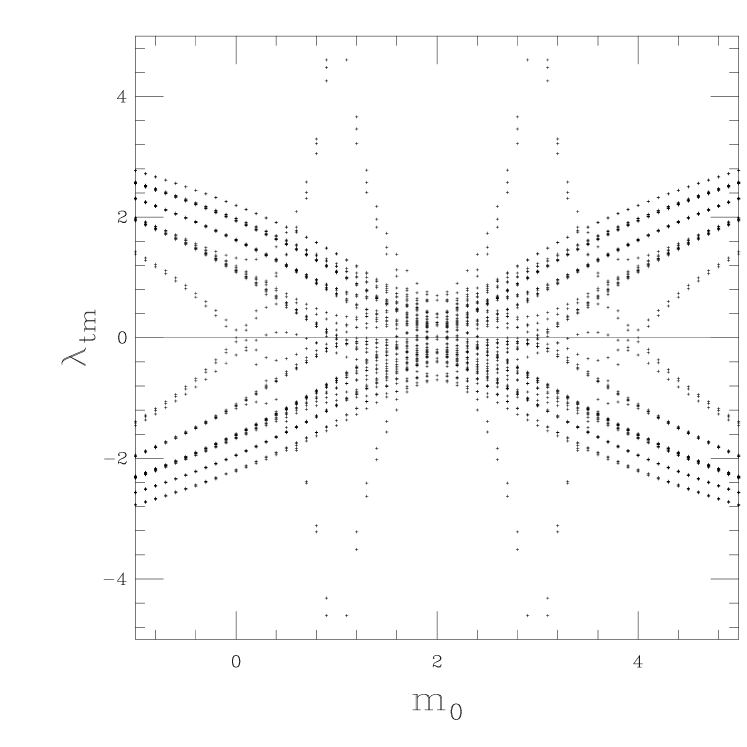
Figure 5: $\lambda_{tm}$ vs. $m_{0}$ for $a_{5}=1$ and an SU(3) “instanton” background (plaquette $\approx 0.05$) on a $2^{4}$ lattice of hypercubes.

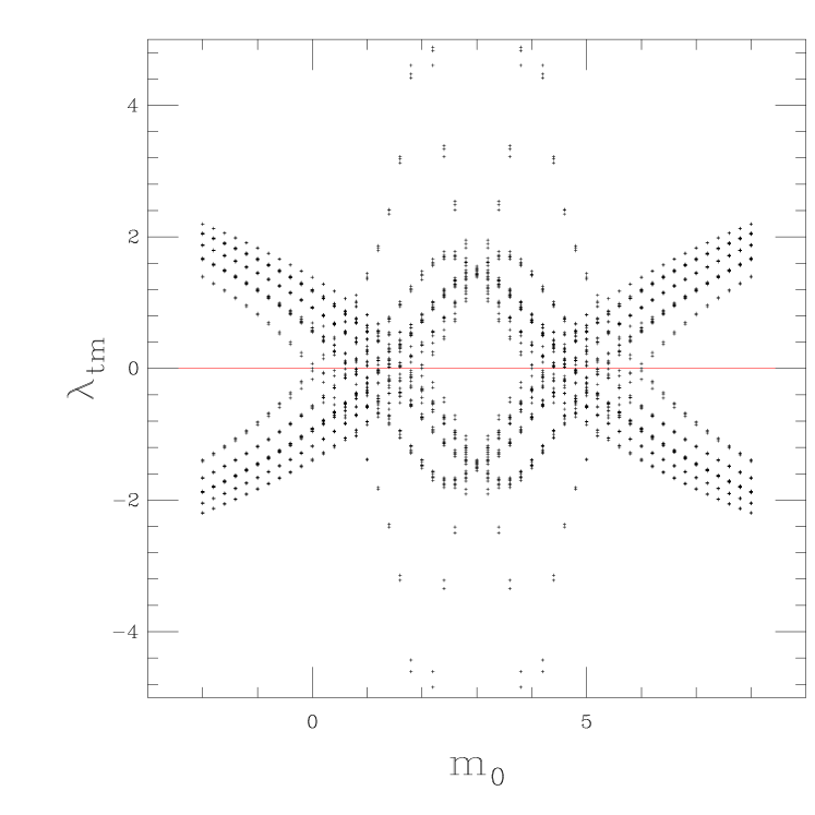
Figure 6: $\lambda_{tm}$ vs. $m_{0}$ for $a_{5}=0.5$ and an SU(3) “instanton” background (plaquette $\approx 0.05$) on a $2^{4}$ lattice of hypercubes.

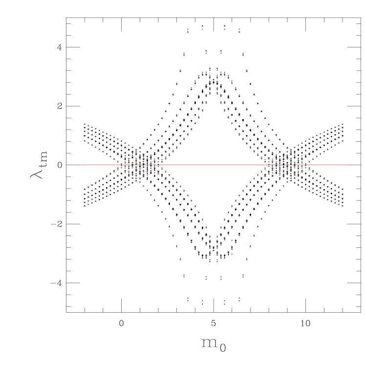
Figure 7: $\lambda_{tm}$ vs. $m_{0}$ for $a_{5}=0.25$ and an SU(3) “instanton” background (plaquette $\approx 0.05$) on a $2^{4}$ lattice of hypercubes.

But this is not all. We had a hard time at first because we used SU(2) gauge fields. And the spectrum was always inexplicably not two-fold but four-fold degenerate, for any gauge field (smooth or rough)! This is the second surprise. And it will not be investigated further here. After all, what good is a paper that does not leave some mystery behind… In any case this property is likely linked to the fact that $-1$ is part of the groups SU(2), SU(4), …but is not part of the group SU(3), etc.

VIII The single component basis and simulating SDWF

In the previous sections we discussed the properties of the SDWF Dirac operator in the basis proposed by the Saclay group. By now, the reader has seen the advantage of this approach in determining the properties of robust zeros of the transfer matrix. In the past, technical problems have disfavored direct simulation of dynamical fermions in this basis in lieu of the simpler single component basis, where there is just a single fermionic spin-flavor degree of freedom per site.

In this section, we will first discuss the construction of the SDWF in the single component basis with an emphasis on preserving, to the maximum extent possible, all of the symmetries of section III. One consequence is that the spin-flavor algebra, i.e. $(\gamma_{5}\otimes\openone)^{2}=(\openone\otimes\openone)$, will be broken and only recovered in the continuum limit. Next, we will discuss a technique where the spin-flavor algebra is restored at the expense of some lattice symmetries. We believe these lattice symmetries can be restored by proper stochastic averaging. Finally, we will discuss a new algorithm based on double regularization for simulating staggered (and SDWF) fermions directly in the Saclay basis. As is typically the case in our field, performance during numerical simulation of QCD will likely determine which of the three proposals survive. We feel that further research in this area is needed.

VIII.1 Single component basis without projection

Let us first review the staggered action in the single component basis and the transformation connecting it to the Saclay basis. From Eqs. (5) through (10), with $m_{0}=1/a_{5}$, the equivalent $2n$ dimensional Dirac operator is usually written

$$D(x,x^{\prime})\chi(x^{\prime})=\frac{1}{2}\sum_{\mu}(-1)^{\hat{\mu}\cdot\eta(x)}\left[U_{\mu}(x)\delta(x+\hat{\mu}-x^{\prime})-U_{\mu}^{\dagger}(x)\delta(x-\hat{\mu}-x^{\prime})\right]\chi(x^{\prime})$$ (65)

with the components of the binary vector $\eta$ given by

$$\eta_{1}(x) = 0,$$

$$\eta_{2}(x) = x_{1}\pmod{2},$$

$$\vdots$$

$$\eta_{2n}(x) = x_{1}+\cdots+x_{2n-1}\pmod{2}.$$ (66)

In the free theory, the unitary transformation from single component site-wise fields $\chi(x)$ to the hypercubic fields $\psi(y)$ is simple. As in section II, if we label sites on the hypercube starting at the origin $O$ by a binary vector $A$ the transformation is

$$\psi_{\alpha a}(y)\propto\Gamma_{\alpha a,A}\chi(2y+O+A)$$ (67)

with the rows of the $2^{2n}\times 2^{2n}$ dimensional matrix $\Gamma$ indexed by the various combinations of spin $\alpha$ and flavor $a$ indices and the columns indexed by the corners of the hypercube $y$. Specifically, the components of the free $\Gamma$ may be chosen as

$$\Gamma_{\alpha a,A}=\left[\gamma_{1}^{A_{1}}\gamma_{2}^{A_{2}}\times\cdots\times\gamma_{2n}^{A_{2n}}\right]_{\alpha a}$$ (68)

where the row index $\alpha$ and column index $a$ of the $2^{n}$ dimensional representation of the Clifford algebra are interpreted as spin and flavor indices.

When the staggered action is made gauge invariant, differences will arise between the two formulations. In the single component basis, fermions are only coupled to nearest neighbor sites, so simple links are all that is needed to preserve gauge invariance. Of course, longer paths could be used to link sites and indeed are often used to implement an improvement program. In the Saclay basis, since fermion fields are associated with hypercubes, the gauge fields must be used to move the components on the hypercube to some common point where the hypercubic field can be assembled. While it may seem that the resulting actions could be completely different, they have the same terms, site by site, that differ only in the choice of paths used to connect nearest neighbors. Hence, they have the same continuum limit.

However, this is not the end of the story. For example, when moving a component two sites on the hypercube for the construction of the hypercubic field there are two equivalent minimum distance paths from which to choose. Choosing one path over the other will preserve the unitarity of $\Gamma$ but break the rotation by $\pi/2$ symmetry. Conversely, choosing to average over both paths preserves rotations but means $\Gamma$ need not be unitary, and thus potentially singular for sufficiently rough gauge fields. For SDWF, some terms in the action may also break the shift by one lattice spacing symmetry. The well known source of the problem is the imposition of the artificial hypercubic structure for the identification of spin and flavor degrees of freedom Mitra and Weisz (1983).

Thus, a conservative approach is to abandon a transcription from hypercubic bases and directly use the single component basis and the technique of Golterman and Smit Golterman and Smit (1984). Using the symmetric shift operator with the binary vector $\zeta(x)$ and scalar $\varepsilon(x)$

$$E_{\mu}(x,x^{\prime})=(-1)^{\hat{\mu}\cdot\zeta(x)}\frac{1}{2}\left[U_{\mu}(x)\delta(x+\hat{\mu}-x^{\prime})+U_{\mu}^{\dagger}(x-\hat{\mu})\delta(x-\hat{\mu}-x^{\prime})\right]$$ (69)

$$\zeta_{1}(x)=x_{2}+\cdots+x_{2n}\pmod{2},\ \cdots,\ \zeta_{2n-1}=x_{2n}\pmod{2},\ \zeta_{2n}=0$$ (70)

$$\varepsilon(x)=x_{1}+\cdots+x_{2n}\pmod{2}$$ (71)

we write the $m_{0}$ term

$$\frac{1}{2}\left(\frac{1}{a_{5}}-m_{0}\right)\sum_{\mu}\left(\gamma_{5}\otimes\xi_{5\mu}\right)\psi(y)\to\frac{1}{2}\left(\frac{1}{a_{5}}-m_{0}\right)(-1)^{\varepsilon(x)}\sum_{\mu}E_{\mu}(x,x^{\prime})\chi(x^{\prime})$$ (72)

and the chiral projection operators are constructed using

$$\left(\gamma_{5}\otimes\openone\right)\psi(y)\to\frac{(-1)^{\varepsilon(x)}}{(2n)!}\sum_{\mu_{1}\cdots\mu_{2n}}\epsilon_{\mu_{1}\cdots\mu_{2n}}E_{\mu_{1}}(x,x^{(1)})\times\cdots\times E_{\mu_{2n}}(x^{(2n-1)},x^{(2n)})\chi(x^{(2n)})$$ (73)

where $\epsilon_{\mu_{1}\cdots\mu_{2n}}$ is the totally antisymmetric tensor and the summation over the $2n$ site vectors $x^{(1)},\cdots,x^{(2n)}$ is implied. The upside to this approach is that it preserves the staggered symmetries to the extent possible. The downside is that chiral projection is no longer exact, except in the continuum limit. Of course, this is a different manifestation of the same problem that makes the transformation to the Saclay basis non-unitary, where projection is exact.

VIII.2 Exact projection with stochastic symmetrization

The second approach addresses the projection problem at the expense of breaking some symmetries, which can be restored in the ensemble average as described below. Our example will use the hypercubic basis of Daniel and Sheard Daniel and Sheard (1988) but equivalent examples are to construct a unitary transformation $\Gamma$ into the Saclay basis or even to restrict the Golterman–Smit operators to single paths between sites.

Quickly reviewing the Daniel–Sheard formulation, we want to construct “local” fermion bilinears of definite spin and flavor, where local means local to the hypercube, from the single component states $\chi(x)$. We identify the hypercubic Daniel–Sheard fields by a simple relabeling: $\chi_{A}(y)=\chi(x)$ and $x=2y+O+A$ as before. Local bilinears are written

$$\overline{\chi}_{A}(y)(\overline{\gamma_{S}\otimes\xi_{F}})_{AB}\chi_{B}(y)=\sum_{x,x^{\prime}}(-1)^{\phi(x,x^{\prime})}\overline{\chi}(x)\mathcal{U}(x,x^{\prime})\chi(x^{\prime})$$ (74)

where $x,x^{\prime}$ are summed over the hypercube and $\mathcal{U}(x,x^{\prime})$ represents the links chosen to make the bilinear gauge invariant. The notation is $\gamma_{S}=\gamma_{1}^{S_{1}}\times\cdots\times\gamma_{2n}^{S_{2n}}$ and the phase factor is computed from

$$(\overline{\gamma_{S}\otimes\xi_{F}})_{AB}\ \Rightarrow\ \phi(A,B)=\frac{1}{2^{n}}\text{Tr}\left(\gamma_{A}^{\dagger}\gamma_{S}\gamma_{B}\gamma_{F}^{\dagger}\right).$$ (75)

As an aside, this gives exactly the same terms appearing in Eqs. (72) and (73) provided you keep only the terms on a single hypercube.

As mentioned before, imposing a hypercubic structure introduces problems with maintaining the staggered symmetries for arbitrary spin and flavor choices. Our proposal is at the beginning of each update step of whatever update algorithm, first choose the origin $O$ at random from the $2^{2n}$ ways of imposing the hypercubic structure on the lattice. Next, choose at random only one of the minimum distance paths on the hypercube for making bilinears gauge invariant with the restriction that the same path is used in both directions. Thus, $\mathcal{U}(A,B)$ is unitary and $\mathcal{U}^{\dagger}(A,B)=\mathcal{U}(B,A)$. Note that different paths can be used on different hypercubes. Choosing a random hypercubic structure and random paths on the hypercubes at each update step ensures that symmetry breaking effects due to these choices will cancel out in the ensemble average. The purpose of choosing only one path per pair of corners on the hypercube is to guarantee the chiral projection property. For example, $(\overline{\gamma_{5}\otimes\openone})^{\dagger}\left[(\overline{\gamma_{5}\otimes\openone})\chi\right]\to\chi$ which is the same as the continuum where we normally choose Hermitian gamma matrices.

VIII.3 Doubly regularized staggered fermions

The third proposal is specific to the Saclay basis but applies equally well to SDWF and staggered fermions with Pauli–Villars fields. Following the second proposal, we can construct at each update step a unitary transformation from the single component basis to the Saclay basis that will certainly depend on the gauge field but not on the value of the mass $m_{f}$. Since the fermionic action and the Pauli–Villars action only differ by the value of $m_{f}$, then the contributions from the transformation will cancel between fermions and the pseudofermions. Specifically, the fermionic partition function on a fixed gauge background and for finite lattice spacing, volume and $L_{s}$ is

$$Z_{\text{F}}\left[U\right] = \int\left[d\overline{\chi}_{\text{F}}d\chi_{\text{F}}\right]\int\left[d\phi_{\text{PV}}^{\dagger}d\phi_{\text{PV}}\right]e^{\overline{\chi}_{\text{F}}\Gamma^{\dagger}D_{\text{F}}(m_{f})\Gamma\chi_{\text{F}}-\phi_{\text{PV}}^{\dagger}\Gamma^{\dagger}D_{\text{F}}(m_{f}=1)\Gamma\phi_{\text{PV}}}$$ (76)

$$= \frac{\det\Gamma^{\dagger}\ \det D_{\text{F}}(m_{f})\ \det\Gamma}{\det\Gamma^{\dagger}\ \det D_{\text{F}}(m_{f}=1)\ \det\Gamma}=\frac{\det D_{\text{F}}(m_{f})}{\det D_{\text{F}}(m_{f}=1)}$$

$$= \int\left[d\overline{\Psi}d\Psi\right]\int\left[d\Phi^{\dagger}d\Phi\right]e^{\overline{\Psi}D_{\text{F}}(m_{f})\Psi-\Phi^{\dagger}D_{\text{F}}(m_{f}=1)\Phi}$$

which is what we had back in Eq. (1). In practice, we do not need to specify the paths chosen for the basis transformation since they cancel from the path integral. But, it would still be important to choose at random the origin $O$ of the hypercubic structure at each update step to avoid violations of the shift by one lattice spacing symmetry. We would like to emphasize again that this proposal should work for staggered fermions with added Pauli–Villars fields and we believe this is another example of the potential of double regularization to improve the usefulness of existing fermion actions by canceling lattice artifacts Fleming (2001a). Also, notice that the number of fermionic degrees of freedom is the same as in the single component basis because the Saclay fields are defined on hypercubes.

Of course, some of the ideas presented in this section for implementing SDWF for numerical simulation have been discussed before, e.g. the idea for stochastic restoration of staggered symmetries is certainly descended from the work of Christ, Freidberg and Lee Christ et al. (1982).

IX Alternative actions

The SDWF action considered here is not unique. It is possible that actions with better scaling properties may be constructed using improved fields in the same spirit as with staggered fermions (see Luo (1997); Lee and Sharpe (1999) and references therein). Additionally, in our earlier work Fleming and Vranas (2002) we introduced the domain wall defect using a local mass term (distance zero) which preserved the shift by one lattice spacing symmetry (among others) and broke the U(1)$\times$U(1) chiral symmetry. In this work, we considered a distance one mass term which preserves the chiral symmetry and breaks the shift symmetry. We view this as a better choice because the additive renormalization it produces Mitra and Weisz (1983) merely contributes to the flavor breaking term that our domain wall formulation is designed to eliminate. It is possible that other distance mass terms might prove useful in the future and even have a faster exponential rate of restoration of flavor symmetry. We emphasize that the primary requirements for these mass terms are that they be of the order of the cutoff and commute with the operators in Eq. (20).

X Conclusions

In this paper a different lattice fermion regulator was presented. Staggered domain wall fermions are defined in $2n+1$ dimensions and describe $2^{n}$ flavors of light lattice fermions with exact U(1)$\times$U(1) chiral symmetry in $2n$ dimensions. The full SU($2^{n}$)$\times$SU($2^{n}$) flavor symmetry is recovered as the size of the extra dimension is increased. SDWF give a different perspective into the inherent flavor mixing of lattice fermions and by design present an advantage for numerical simulations of lattice QCD thermodynamics. We have paid particular attention to the chiral and topological index properties of the SDWF Dirac operator and its associated transfer matrix. In the limit where the lattice spacing in the extra dimension $a_{5}$ tends to zero the corresponding Hamiltonian $H_{0}$ is proportional to the identity in flavor space illustrating the complete absence of flavor mixing.

For a semi-infinite extent in the extra dimension, the theory has four chiral fermions with the same chiral charges and is anomalous. To construct an anomaly free theory, we must use such “quadruplets” with charges as dictated by the corresponding anomaly cancellation condition. This is completely analogous to the case of Wilson DWF.

However, there are still a number of unresolved issues related to this formulation which need to be studied in future work. In particular:

1. For QCD, the nearly four-fold crossing degeneracy of the Hamiltonian must be investigated thoroughly.

2. SDWF should be implemented for numerical simulation according to the proposals of section VIII. In the broken phase of QCD, it is obviously important to confirm that one pion is a pseudo-Goldstone boson and that the remaining fourteen non-singlet pions become degenerate with the pseudo-Goldstone boson as $L_{s}\to\infty$. Also, the expected robustness of topological zero modes should be confirmed as was done for DWF Chen et al. (1999).

3. We have presented an analysis of the zeros of the SDWF Hamiltonian through the pseudo-Hamiltonian $H_{p}$ and in the limit $a_{5}\to 0$ where the flavor breaking is trivially absent in $H_{0}$. A derivation and analysis of the full spectrum of the Hamiltonian for general $a_{5}$ is needed.

4. Since the nearly degenerate four-fold crossings in the spectrum of the Hamiltonian have the same chiral charge, the conserved currents of the full SU($2^{n}$)$\times$SU($2^{n}$) symmetry must exist and can be constructed in the overlap formalism Narayanan and Neuberger (1995). Simpler constructions of these currents may be possible. Constructing and measuring the conservation of these currents in simulations is important.

5. SDWF were constructed with the simulation of QCD thermodynamics in mind because of the importance of having a continuous subgroup of chiral symmetry for any $L_{s}$. It is worth confirming that this gives SDWF some advantage over DWF in looking for critical fluctuations at the finite temperature QCD phase transition.

6. It would be very interesting to add the Kogut-Sinclair four-fermion interaction Kogut and Sinclair (1997); Kogut et al. (1998) to the SDWF action to enable simulation at zero quark mass in the region of the QCD phase transition.

7. The domain wall mass term must be of the order of the lattice spacing and will introduce a hard breaking of some part of the staggered symmetry group, in our case the shift by one lattice spacing symmetry, causing quantum corrections to the SDWF transfer matrix Mitra and Weisz (1983). Our analysis of the transfer matrix spectrum indicates a range of $m_{0}$ values can still be found where the transfer matrix behaves correctly in the presence of gauge field topology, as was the case with Wilson DWF. We believe this issue should be studied thoroughly.

8. Can SDWF reveal (or has it already revealed) some new insight into the nature of inherent flavor mixing of lattice fermions?

On the strength of the results of our transfer matrix analysis, we believe that SDWF may be an attractive alternative to DWF. The formulation is now sufficiently mature that the issues above should now be addressed in the context of QCD. As has been the case with staggered and Wilson fermions in the past, we should have a choice between SDWF and DWF for a given problem according to our resources and preference in the near future.

References

- Kaplan (1992) D. B. Kaplan, Phys. Lett. B288, 342 (1992), eprint [http://arXiv.org/abs]hep-lat/9206013.
- Kaplan (1993) D. B. Kaplan, Nucl. Phys. Proc. Suppl. 30, 597 (1993).
- Narayanan and Neuberger (1993a) R. Narayanan and H. Neuberger, Phys. Lett. B302, 62 (1993a), eprint [http://arXiv.org/abs]hep-lat/9212019.
- Narayanan and Neuberger (1994a) R. Narayanan and H. Neuberger, Nucl. Phys. B412, 574 (1994a), eprint [http://arXiv.org/abs]hep-lat/9307006.
- Frolov and Slavnov (1993) S. A. Frolov and A. A. Slavnov, Phys. Lett. B309, 344 (1993).
- Frolov and Slavnov (1994) S. A. Frolov and A. A. Slavnov, Nucl. Phys. B411, 647 (1994), eprint [http://arXiv.org/abs]hep-lat/9303004.
- Kikukawa (2002) Y. Kikukawa, Nucl. Phys. Proc. Suppl. 106, 71 (2002), eprint [http://arXiv.org/abs]hep-lat/0111035.
- Edwards (2002) R. G. Edwards, Nucl. Phys. Proc. Suppl. 106, 38 (2002), eprint [http://arXiv.org/abs]hep-lat/0111009.
- Vranas (2001) P. M. Vranas, Nucl. Phys. Proc. Suppl. 94, 177 (2001), eprint [http://arXiv.org/abs]hep-lat/0011066.
- Golterman (2001) M. Golterman, Nucl. Phys. Proc. Suppl. 94, 189 (2001), eprint [http://arXiv.org/abs]hep-lat/0011027.
- Neuberger (2000) H. Neuberger, Nucl. Phys. Proc. Suppl. 83, 67 (2000), eprint [http://arXiv.org/abs]hep-lat/9909042.
- Luscher (2000) M. Luscher, Nucl. Phys. Proc. Suppl. 83, 34 (2000), eprint [http://arXiv.org/abs]hep-lat/9909150.
- Blum (1999) T. Blum, Nucl. Phys. Proc. Suppl. 73, 167 (1999), eprint [http://arXiv.org/abs]hep-lat/9810017.
- Shamir (1996) Y. Shamir, Nucl. Phys. Proc. Suppl. 47, 212 (1996), eprint [http://arXiv.org/abs]hep-lat/9509023.
- Creutz (1995) M. Creutz, Nucl. Phys. Proc. Suppl. 42, 56 (1995), eprint [http://arXiv.org/abs]hep-lat/9411033.
- Narayanan and Neuberger (1994b) R. Narayanan and H. Neuberger, Nucl. Phys. Proc. Suppl. 34, 587 (1994b), eprint [http://arXiv.org/abs]hep-lat/9311015.
- Wilson (1977) K. G. Wilson, in New Phenomena in Subnuclear Physics, Part A, edited by A. Zichichi (Plenum Press, New York, 1977), vol. 13 of The Subnuclear Series, pp. 69–125, ISBN 0-306-38181-8 (part A), proceedings of the first half of the 1975 International School of Subnuclear Physics, Erice, Sicily, July 11 - August 1, 1975, CLNS-321.
- Shamir (1993) Y. Shamir, Nucl. Phys. B406, 90 (1993), eprint [http://arXiv.org/abs]hep-lat/9303005.
- Kogut and Susskind (1975) J. B. Kogut and L. Susskind, Phys. Rev. D11, 395 (1975).
- Banks et al. (1976) T. Banks, L. Susskind, and J. B. Kogut, Phys. Rev. D13, 1043 (1976).
- Susskind (1977) L. Susskind, Phys. Rev. D16, 3031 (1977).
- Fleming and Vranas (2002) G. T. Fleming and P. M. Vranas, Nucl. Phys. Proc. Suppl. 106, 724 (2002), eprint [http://arXiv.org/abs]hep-lat/0110172.
- Vranas (2000) P. M. Vranas, Nucl. Phys. Proc. Suppl. 83, 414 (2000), eprint [http://arXiv.org/abs]hep-lat/9911002.
- Chen et al. (2001) P. Chen et al., Phys. Rev. D64, 014503 (2001), eprint [http://arXiv.org/abs]hep-lat/0006010.
- Fleming (2001a) G. T. Fleming, Nucl. Phys. Proc. Suppl. 94, 393 (2001a), eprint [http://arXiv.org/abs]hep-lat/0011069.
- Fleming (2001b) G. T. Fleming, Ph.D. thesis, Columbia University, New York (2001b), uMI-99-98152.
- Kluberg-Stern et al. (1983) H. Kluberg-Stern, A. Morel, O. Napoly, and B. Petersson, Nucl. Phys. B220, 447 (1983).
- Gliozzi (1982) F. Gliozzi, Nucl. Phys. B204, 419 (1982).
- van den Doel and Smit (1983) C. van den Doel and J. Smit, Nucl. Phys. B228, 122 (1983).
- Golterman and Smit (1984) M. F. L. Golterman and J. Smit, Nucl. Phys. B245, 61 (1984).
- Daniel and Sheard (1988) D. Daniel and S. N. Sheard, Nucl. Phys. B302, 471 (1988).
- Narayanan and Neuberger (1993b) R. Narayanan and H. Neuberger, Phys. Rev. Lett. 71, 3251 (1993b), eprint [http://arXiv.org/abs]hep-lat/9308011.
- Narayanan and Neuberger (1995) R. Narayanan and H. Neuberger, Nucl. Phys. B443, 305 (1995), eprint [http://arXiv.org/abs]hep-th/9411108.
- Vranas (1997) P. M. Vranas, Nucl. Phys. Proc. Suppl. 53, 278 (1997), eprint [http://arXiv.org/abs]hep-lat/9608078.
- Vranas (1998) P. M. Vranas, Phys. Rev. D57, 1415 (1998), eprint [http://arXiv.org/abs]hep-lat/9705023.
- Jolicoeur et al. (1986) T. Jolicoeur, A. Morel, and B. Petersson, Nucl. Phys. B274, 225 (1986).
- Mitra and Weisz (1983) P. Mitra and P. Weisz, Phys. Lett. B126, 355 (1983).
- Neuberger (1998) H. Neuberger, Phys. Rev. D57, 5417 (1998), eprint [http://arXiv.org/abs]hep-lat/9710089.
- Christ et al. (1982) N. H. Christ, R. Friedberg, and T. D. Lee, Nucl. Phys. B202, 89 (1982).
- Luo (1997) Y. Luo, Phys. Rev. D55, 353 (1997), eprint [http://arXiv.org/abs]hep-lat/9604025.
- Lee and Sharpe (1999) W. Lee and S. R. Sharpe, Phys. Rev. D60, 114503 (1999), eprint [http://arXiv.org/abs]hep-lat/9905023.
- Chen et al. (1999) P. Chen et al., Phys. Rev. D59, 054508 (1999), eprint [http://arXiv.org/abs]hep-lat/9807029.
- Kogut and Sinclair (1997) J. B. Kogut and D. K. Sinclair, Nucl. Phys. Proc. Suppl. 53, 272 (1997), eprint [http://arXiv.org/abs]hep-lat/9607083.
- Kogut et al. (1998) J. B. Kogut, J. F. Lagae, and D. K. Sinclair, Phys. Rev. D58, 034504 (1998), eprint [http://arXiv.org/abs]hep-lat/9801019.