[

Probing hadron wave functions in Lattice QCD

C. Alexandrou

Department of Physics, University of Cyprus, P.O. Box 20537, CY-1678 Nicosia, Cyprus

Ph. de Forcrand

Institute für Theoretische Physik, ETH Hönggerberg, CH-8093 Zürich, Switzerland
and CERN, Theory Division, CH-1211 Geneva 23, Switzerland

A. Tsapalis

Department of Physics, University of Wuppertal, Wuppertal, Germany

(June 20, 2002)

Gauge-invariant equal-time correlation functions are calculated in lattice QCD within the quenched approximation and with two dynamical quark species. These correlators provide information on the shape and multipole moments of the pion, the rho, the nucleon and the $\Delta$.

PACS numbers: 11.15.Ha, 12.38.Gc, 12.38.Aw, 12.38.-t, 14.70.Dj

]

I Introduction

State of the art lattice calculations of hadronic matrix elements have produced very accurate spectroscopic information. Examples of the accuracy reached in quenched lattice QCD are the calculation of the masses of low lying hadrons [1] and glueballs [2]. However progress in determining hadron wave functions and quark distributions has not been so rapid. The initial calculations of Bethe-Salpeter amplitudes were carried out on a rather small lattice in the mid 80’s [3] for the pion and the rho. Further progress came in the early 90’s when the Bethe-Salpeter amplitudes were calculated on a larger lattice for the pion and the rho [4, 5] as well as for the nucleon and the $\Delta$ [4]. However the results were of limited interest because of their manifest dependence on the gauge chosen. A different approach to explore hadronic structure was pursued by the authors of refs. [6]; instead of fixing a gauge or a path for the gluons, they considered correlation functions of quark densities which, being expectation values of local operators, are gauge invariant. This is the approach we have adopted in this work.

Our main motivation for studying density correlators is that they reduce, in the non-relativistic limit, to the wave function squared and thus they provide detailed, gauge-invariant information on hadron structure. The shape of hadrons is one such important quantity that can be directly studied. The issue whether the nucleon is deformed from a spherical shape was raised twenty years ago [7] and is still unsettled. Because the spectroscopic quadrupole moment of a spin one-half particle vanishes, in experimental studies one searches for quadrupole strength in the $\gamma^{*}N\>\rightarrow\>\Delta$ transition. Spin-parity selection rules allow a magnetic dipole, M1, an electric quadrupole, E2, or a Coulomb quadrupole, C2, amplitude. If both the nucleon and the $\Delta$ are spherical then the electric and Coulomb quadrupole amplitudes are expected to be zero. Although M1 is indeed the dominant amplitude there is mounting experimental evidence that E2 and C2 are non-zero. The physical origin of a non-zero E2 and C2 amplitude is attributed to different mechanisms in the various models. In quark models the deformation is due to the colour-magnetic tensor force[7]. In “cloudy” baryon models it is due to meson exchange currents [8].

A recent experimental search at $q^{2}=0.126$ GeV² has yielded an electric quadrupole to magnetic dipole amplitude ratio [9]:

$$R_{EM}={\cal G}_{E2}/{\cal G}_{M1}=(-2.1\pm 0.2\pm 2.0)\%\quad.$$ (1)

The larger error, an order of magnitude larger than the statistical error, is due to the model dependence in the extraction of this ratio from the experimental data. The experimental determination of $R_{EM}$ is complicated by the presence of nonresonant processes coherent with the resonant excitation of $\Delta(1232)$.

The ratio $R_{EM}$ can be evaluated within lattice QCD without any model assumptions by computing the transition matrix element $N$ to $\Delta$. An early lattice calculation of this transition matrix element provided an estimate of $R_{EM}=(-3\pm 8)\%$  [10].

Here we consider an alternative route to understanding the issue of deformation, via the direct study of hadron wave functions. We compute density-density correlators for mesons and baryons and three-density correlators for baryons and look for asymmetries when these are projected along the spin axis or perpendicular to it. The observables that we use are described in section II. In section III we give the relations for the deformation among the states of different spin projections. Our quenched lattice results are presented in section IV. They clearly give support to a deformed rho. The nucleon deformation averages to zero in agreement with the fact that its spectroscopic quadrupole moment is zero. An analysis of the intrinsic nucleon deformation requires determining the body-fixed coordinates by diagonalization of the moment of inertia tensor, which must be done configuration by configuration. This is too noisy to yield a statistically significant result. On the other hand the $\Delta$ has a non zero spectroscopic moment and any deformation should be detected via projection with respect to its spin axis. In quenched QCD we detect no significant deformation for the $\Delta$ within our present statistics.

In addition to providing information about deformation, baryon wave functions, calculated for the first time in a gauge invariant way for all values of the relative coordinates, can be used to study indirectly the potential among the three quarks. By performing fits to the three-density correlators, we find that a reasonable ansatz for the baryonic potential is provided by the sum of two-body potentials, called the $\Delta$-Ansatz [11].

Comparison between quenched and full QCD results sheds light on the role of the pion cloud. It is known that quenching eliminates all or part of the pion cloud depending on the hadronic state. For the rho channel no intermediate backgoing quarks with the pion quantum numbers are present [12], so the deformation that we observe is not due to the pion cloud. We use the SESAM configurations [13] to investigate unquenching effects. We find that the deformation in the rho increases. We detect a deformation in the $\Delta$ which remains small for the values of the dynamical quark mass considered. The unquenched lattice results are presented in section V. Section VI contains our conclusions.

II Correlation functions

The wave function of a meson is usually defined in a given gauge $g$ as the equal time Bethe-Salpeter amplitude

$$\Phi^{\rm BS}_{g}({\bf r})=\int d^{3}r^{\prime}<0|\bar{q}^{f_{1}}({\bf r}^{\prime})\Gamma q^{f_{2}}({\bf r}^{\prime}+{\bf r})|M>$$ (2)

where $\Gamma$ is a Dirac matrix with the quantum numbers of the meson $M$ of flavor $f_{1},f_{2}$. $\Phi^{\rm BS}_{g}({\bf r})$ is the minimal Fock space state wave function, which is an approximation to the full wave function since other multiquark components are excluded. For the Bethe-Salpeter amplitude one must either fix the gauge or connect the quarks with gluons to form gauge-invariant (but path-dependent) quantities. Wave functions for baryons are defined in an analogous way to the meson wave functions but they involve two relative distances. E.g. the Bethe-Salpeter amplitude, $\Phi^{\rm BS}_{g}({\bf r}_{1},{\bf r}_{2})$, for the proton is given by

$$\sum_{\bf r^{\prime}}<0|\epsilon^{abc}u^{a}_{\delta}({\bf r}^{\prime},t)\biggl{(}u^{b\>T}({\bf r}^{\prime}+{\bf r}_{1},t)\>C\gamma_{5}\>d^{c}({\bf r}^{\prime}+{\bf r}_{2},t)\biggr{)}|B>\quad.$$ (3)

Summation over ${\bf r}^{\prime}$ projects onto zero momentum. For the $\Delta^{+}$, the interpolating field that we take is

$$J_{\mu}({\bf x}) = \frac{\epsilon^{abc}}{\sqrt{3}}\Biggl{[}u^{a}({\bf x})\biggl{(}2u^{b\>T}({\bf x})\>C\gamma_{\mu}d^{c}({\bf x})\biggr{)}$$ (4)

$$+ d^{a}({\bf x})\biggl{(}u^{b\>T}({\bf x})\>C\gamma_{\mu}u^{c}({\bf x})\biggr{)}\Biggl{]}\quad,$$ (5)

where $C=\gamma_{0}\gamma_{2}$ is the charge conjugation operator. We use $\Gamma_{\pm}=(\gamma_{1}\mp i\gamma_{2})/2$ to create a hadron of a definite spin component $J_{z}$. Explicitly for the first term in Eq. 5 we take

$$J_{3/2} : \frac{\epsilon^{abc}}{\sqrt{3}}\Biggl{[}u^{a}_{1}({\bf x})\biggl{(}2u^{b\>T}({\bf x})\>C\Gamma_{+}d^{c}({\bf x})\biggr{)}\Biggr{]}$$ (6)

$$J_{1/2} : \frac{\epsilon^{abc}}{\sqrt{3}}\Biggl{[}u^{a}_{1}({\bf x})\biggl{(}2u^{b\>T}({\bf x})\>C\gamma_{3}d^{c}({\bf x})\biggr{)}$$ (8)

$$-u^{a}_{2}({\bf x})\biggl{(}2u^{b\>T}({\bf x})\>C\Gamma_{+}d^{c}({\bf x})\biggr{)}\Biggr{]}$$

$$J_{-1/2} : \frac{\epsilon^{abc}}{\sqrt{3}}\Biggl{[}u^{a}_{2}({\bf x})\biggl{(}2u^{b\>T}({\bf x})\>C\gamma_{3}d^{c}({\bf x})\biggr{)}$$ (10)

$$+u^{a}_{1}({\bf x})\biggl{(}2u^{b\>T}({\bf x})\>C\Gamma_{-}d^{c}({\bf x})\biggr{)}\Biggr{]}$$

$$J_{-3/2} : \frac{\epsilon^{abc}}{\sqrt{3}}\Biggl{[}u^{a}_{2}({\bf x})\biggl{(}2u^{b\>T}({\bf x})\>C\Gamma_{-}d^{c}({\bf x})\biggr{)}\Biggr{]}\quad.$$ (11)

where $q_{i}$ is the $i$th component of the spinor. The same construction is done for the second term of Eq. 5. With these combinations we recover, in the non-relativistic limit, the quark model wave functions of these states.

The Bethe-Salpeter amplitudes in the Coulomb and in the Landau gauge were investigated in ref. [4]. Instead of fixing a gauge, a gauge-invariant wave function, which corresponds to the Bethe-Salpeter amplitude in the axial gauge, can be constructed by joining the quark and the antiquark with a thin string of glue [14]:

$$\psi_{s}(y)=\bigl{\langle}0\bigl{|}\bar{q}(0)\Gamma e^{i\int^{y}_{0}dzA_{y}(z)}q(y)\bigr{|}M\bigr{\rangle}\quad.$$ (12)

Other variations to the thin string are to smear the gluons [5] or to evolve them so that they reach their ground state distribution. It was shown in ref. [14] that there is a much larger probability to find a quark-antiquark pair separated by, say, 1 fm when connected by a physical adiabatic flux tube than when the quarks are surrounded by gluons fixed to the Coulomb gauge or when they are connected by a thin string of gluons. Although in ref. [14] only mesonic states were considered, generalization to baryons is straightforward, with the gluonic strings attached to each of the three quarks contracted at a point.

In this work we opt for the calculation of density-density correlators [15, 16],

$$C({\bf r},t_{1},t_{2})=\int\>d^{3}r^{\prime}\>\langle h|\rho^{u}({\bf r}^{\prime}+{\bf r},t_{2})\rho^{d}({\bf r}^{\prime},t_{1})|h\rangle$$ (13)

where the density operator is given by the normal order product

$$\rho^{u}({\bf r},t)=:\bar{u}({\bf r},t)\gamma_{0}u({\bf r},t):$$ (14)

so that disconnected graphs are excluded.

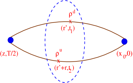
FIG. 1.: Density-density correlator for a meson. $t_{1}$, $t_{2}$, $T/2-t_{1}$ and $T/2-t_{2}$ are taken large enough to isolate the mesonic groundstate.

For mesons the density-density correlator is shown schematically in Fig. 1. Inserting a complete set of hadronic states we find

$$C({\bf r},t_{1},t_{2}) = \sum_{n_{i},n_{f},n}\sum_{\bf{p},\bf{q}}\langle h|n_{f},{\bf{p}}\rangle\frac{e^{-E_{n_{f}}({\bf p})(T/2-t_{2})}}{E_{n_{f}}({\bf p})}$$ (15)

$$\langle n_{f},{\bf p}|\rho^{u}|n,{\bf p}+{\bf q}\rangle e^{-i{\bf q.r}}\frac{e^{-E_{n}({\bf p}+{\bf q})(t_{2}-t_{1})}}{E_{n}({\bf p}+{\bf q})}$$ (16)

$$\langle n,{{\bf p}+{\bf q}}|\rho^{d}|n_{i},{{\bf p}}\rangle\frac{e^{-E_{n_{i}}({\bf p})t_{1}}}{E_{n_{i}}({\bf p})}\langle n_{i},{\bf p}|h\rangle\quad.$$ (17)

The sum over all excitations of the initial, $n_{i}$, and final, $n_{f}$, states yields the ground state hadron in the limit $(T/2-t_{2})\rightarrow\infty$ and $t_{1}\rightarrow\infty$, where $T$ is the lattice extent in Euclidean time. Since we take periodic boundary conditions the maximum time separation is $T/2$. Enforcing zero momentum would require a summation over the spatial volume on the source or sink site. This is technically not feasible since it involves quark propagators from all to all spatial lattice sites. Instead, the suppression of the non-zero momenta and other higher excitations is obtained by choosing the largest possible time separation from the source and the sink. We take the same spatial coordinate for the source and the sink, namely ${\bf x}_{0}={\bf z}$. As a starting point we take, in this work, density insertions to be always at equal times. A disadvantage of the density-density correlators is that they are subject to more severe finite size effects, having typically larger spatial extent ($\sim$ twice) than Bethe-Salpeter amplitudes [6].

In the case of baryons three density insertions are needed and the correlator is given by

$$C({\bf r}_{1},{\bf r}_{2},t)=\int d^{3}r^{\prime}\>\langle h|\rho^{d}({\bf r^{\prime}},t)\rho^{u}({\bf r}^{\prime}+{\bf r}_{1},t)\rho^{u}({\bf r}^{\prime}+{\bf r}_{2},t)|h\rangle$$ (18)

where we have taken all the density insertions to be at equal times. This involves two relative distances. Like (13), it can be computed efficiently by Fast Fourier Transform (FFT).

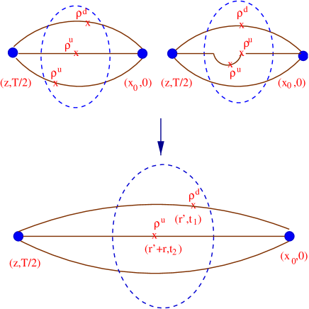
FIG. 2.: The upper two diagrams show the three-density correlator for a baryon as defined in Eq. 18. As in Fig. 1 the density operators are inserted far enough from the source and the sink so that the baryonic groundstate of interest is isolated. The lower diagram shows the equivalent two-density correlator after integration of one of the relative distances.

The relevant diagrams are shown in the upper part of Fig. 2 for the nucleon or the $\Delta^{+}$, for the general case of density insertions at three unequal times. In addition to one density insertion for each $u$-quark line, one can have two density insertions on the same $u$-quark line. Evaluation of this second diagram requires the quark propagator $G({\bf r}_{2},{\bf r}_{1})$ for all partial distances of the two arguments. This is beyond our present resources, and this diagram is not included. To check that the first diagram that we calculate provides by itself a reasonable description of the baryon wave function, we also compute the baryon wave function with two density insertions for the $u$ and $d$ quarks as shown in the lower part of Fig. 2. This may be viewed as the square of the one-particle wave function obtained from the full wavefunction by integrating over one relative coordinate. If the contribution of the second diagram is small then we expect that

$$\int d^{3}r_{2}C({\bf r}_{1},{\bf r}_{2},t)\sim\int\>d^{3}r^{\prime}\>\langle h|\rho^{d}({\bf r}^{\prime},t)\rho^{u}({\bf r}^{\prime}+{\bf r}_{1},t)|h\rangle$$ (19)

will be satisfied, even when the l.h.s of the equation is calculated using only the diagram with one density insertion on each quark line. This comparison will be performed in Sec.IV, B.

III Relations among the deformations in different channels

The interpolating field for a rho meson is taken to be $J_{\mu}(x)=\bar{d}(x)\gamma_{\mu}u(x)$. The physical states of spin projections $0$ and $\pm 1$ for the rho are obtained using interpolating fields $J_{0}(x)=\bar{d}(x)\gamma_{3}u(x)$ and $J_{\pm}=\bar{d}(x)\left[(\gamma_{1}\mp i\gamma_{2})/2\right]u(x)$ respectively. Due to rotational invariance the correlator

$$C_{ss}({\bf r})=\sum_{{\bf x}}\langle J_{s}({\bf z})\rho^{d}({\bf x})\>\rho^{u}({\bf x+r})J_{s}^{\dagger}({\bf 0})\rangle$$ (20)

satisfies the relation $C_{11}({\bf r.\hat{e}_{1}})=C_{22}({\bf r.\hat{e}_{2}})=C_{33}({\bf r.\hat{e}_{3}})$ where $\hat{\bf e}_{j}$ is a unit vector along the $j$-axis. This means that for the $\pm 1$ channels we have $(C_{--}+C_{++})/2=C_{11}+C_{22}$. Due to parity symmetry $C_{--}=C_{++}$ which is satisfied after ensemble averaging and leads to the relations

$$C_{++}=C_{--}=C_{11}+C_{22}\quad.$$ (21)

If we denote by $T(r)$ the tranverse and by $L(r)$ the longitudinal projection of $C_{33}(r)$ with respect to the spin axis, the deformation $\alpha(r)$ is defined by $L(r)/T(r)=1+\alpha(r)$. The deformation in the $\pm 1$ channels is then $2T(r)/(T(r)+L(r))\sim 1-\alpha(r)/2$ for small $\alpha$ i.e if the spin-0 state of the rho is elongated (prolate) along the $z$-axis then the spin $\pm 1$ states will be “flat” (oblate) by approximately half this amount. This observation is consistent with the data shown in Fig. 3.

Non-relativistically one can use the Wigner-Eckart theorem to obtain a similar result. The deformation is obtained by measuring the quadrupole moment defined by

$$Q = \langle JM|2(z^{2}-\frac{x^{2}+y^{2}}{2})|JM\rangle$$ (22)

$$= \sqrt{\frac{4\pi}{5}}\langle JM|2r^{2}Y_{20}(\theta,\phi)|JM\rangle$$ (23)

$$= (-)^{J-M}{J\>\>2\>J\choose-M\>0\>M}\langle J|2r^{2}P_{2}(cos(\theta))|J\rangle$$ (24)

for a state $|JM\rangle$ where J is the spin of the state, M the spin projection along the $z$-axis and ${J\>\>2\>\>J\choose-M\>0\>M}$ is the 3-j symbol. Therefore if we know the deformation for one spin projection we can relate it to the rest. Evaluating the 3-j symbol for the quantum numbers of the rho we find that the deformation for $M=0$ is twice and opposite in sign to that for $M=\pm 1$. We will thus only show results for the spin-0 state, which exhibits the largest deformation.

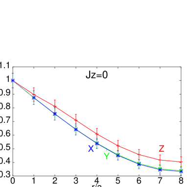
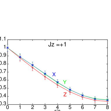
FIG. 3.: Density-density correlator for the rho in a definite spin state $J_{z}=0$ (top) and $J_{z}=+1$ (bottom), for quark separations transverse (line with Z label) and longitudinal (line with X and Y labels) with respect to the spin axis. The hopping parameter is $\kappa=0.154$.

The interpolating fields for projecting to the physical $\Delta^{+}$ spin states were given in Eq. 5. Just like for the deformation of the rho in different spin projections, similar relations can be obtained for the physical components of the $\Delta^{+}$. The interpolating fields for positive spin projections $3/2$ and $1/2$ are no longer related to the negative ones since they involve different spinor components. However the cross terms of the type $\gamma_{1}\gamma_{2}$ contribute an order of magnitude less to the correlator and if we neglect these terms we find for the density-density correlator of the $\pm 3/2$ state that $C_{3/2}\sim C_{-3/2}\sim 1-\alpha(r)/2$ where $\alpha(r)$ is the deformation if we take $\gamma_{3}$ in Eq. 5.

A relation among all the spin projections of the $\Delta^{+}$ can be obtained in the non-relativistic limit by applying the Wigner-Eckart theorem Eq. 24. We find that the deformation for the $M=\pm 3/2$ states is equal and opposite to that for the $M=\pm 1/2$. Among the physical states we will therefore show results only for the $+3/2$. Since we expect the deformation to be maximal when a $\gamma_{3}$ is used in Eq. 5 for the interpolating field, we will also look for deformation in this channel in addition to the $+3/2$ physical state. In the unquenched data where we observe a small deformation these relations between the various amplitudes, as far as the relative signs are concerned, are indeed satisfied.

IV Quenched Lattice results

A Density-density correlation functions

We have analysed 220 quenched configurations at $\beta=6.0$ for a lattice of size $16^{3}\times 32$ obtained from the NERSC archive [17], using the Wilson Dirac operator with hopping parameter $\kappa=0.15,0.153,0.154$ and $0.155$. The ratio of the pion mass to the rho mass at these values of $\kappa$ is $0.88,\>0.84,\>0.78$ and 0.70 respectively. Using the relation $2am_{q}=1/\kappa-1/\kappa_{c}$, with the critical value $\kappa_{c}=0.1571$, we obtain for the naive quark mass $m_{q}$ values of about 300, 170, 130 and 90 MeV respectively, where we used $a^{-1}=1.94$ GeV ($a=0.103$ fm) from the string tension [18] to set the scale. Alternatively, the scale could be set from the rho mass in the chiral limit. This approach yields $a^{-1}$=2.3 GeV ($a=0.087$ fm) [19, 20], with a systematic error of about 10% coming from the choice of fitting range and chiral extrapolation ansatz, which is about twice as large as the statistical one [19]. We note that although that these simulations used the lattices of increasing bigger volumes the scale was not affected. In our discussion of quenched data we will use the value of $a$ determined from the string tension. However, to compare the quenched with the unquenched results we will use the value extracted from the rho mass in the chiral limit since this determination is applicable both in the quenched and in the unquenched theory.

We fix the source and the sink for maximum separation at $t_{i}=a$ and $t_{f}=17a$, where $a$ is the lattice spacing. The density insertions are taken in the middle of the time interval i.e. at $t=9a$. To check that the time interval $|t-t_{i}|=|t-t_{f}|=8a$ is sufficient, we have performed an analysis on 27 configurations at $\kappa=0.153$, varying the time $t$ where the density operators are inserted.

The results for the rho correlator are shown in Fig. 4(a) for four different insertion times at $\kappa=0.153$. As can be seen, density insertions at $t=8a$ and $9a$ give the same correlator, reassuring us that the time separation is large enough to isolate the groundstate of the rho. In the other channels the results are similar, with larger statistical noise for the baryons. In Fig. 4(b) we show in addition the correlator for the spin-0 state of the rho, for quark separations along the spin axis ($z$) and perpendicular to it ($x$). As expected, the deformation is the same when measured from density insertions at $t=8a$ and $t=9a$, since the groundstate is isolated by then. More surprisingly, this $z-x$ asymmetry is almost unchanged when measured at $t=4a$, even though the $z$- and $x$-profiles change appreciably. These findings indicate that the deformation which we observe in more detail below is a robust, physical property of the rho meson in its groundstate as well as its low-lying excited states.

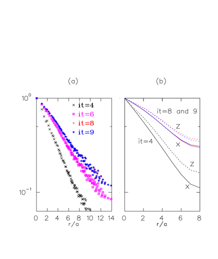
FIG. 4.: (a) The density-density correlator for the rho, measured from density insertions at time $9a,8a,6a$ and $4a$. To avoid cluttering, the data as a function of $r$ are averaged over bins of size $\Delta r=0.07a$. (b) The density-density correlator for the rho, measured from density insertions at time $9a,8a$ and $4a$, for quark separations along the $z$- and $x$-axes. In both cases, 27 configurations are used, and statistical error bars are omitted for clarity.

In Fig. 5 we collect the correlators for the pion, the rho, the nucleon and the $\Delta^{+}$ for the four different quark masses ($\kappa$ values) considered. We confirm an observation made in earlier studies [3, 4] that the wave functions are not very sensitive to the bare quark mass. This behaviour is as expected in the bag model, but is inconsistent with nonrelativistic quark models where a much stronger mass dependence is predicted. Insensitivity on the bare mass can be understood from the consideration that the quarks are dressed and their effective mass is therefore not very much affected by changing the bare mass. From Fig. 5 we also see that the rho wavefunction depends more on the quark mass than the other three. In particular the nucleon and $\Delta^{+}$ wave functions hardly change as we go from $\kappa=0.154$ to $\kappa=0.155$ which corresponds to reducing the naive quark mass from $m_{q}\sim 130$ MeV to $m_{q}\sim 90$ MeV.

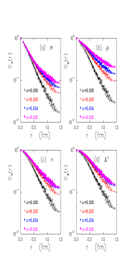
FIG. 5.: Density-density correlators, $C({\bf r})$, for (a) the pion, (b) the rho, (c) the nucleon and (d) the $\Delta^{+}$ versus $|{\bf r}|$ at $\kappa=0.15,0.153,0.154$ and $0.155$. Errors bars are omitted for clarity.

A direct comparison of the sizes of the four hadrons can be made in Fig. 6(a) where we plot the density-density correlators for $\kappa=0.154$. The pion has the smallest size, approximately half that of the $\Delta$, whereas the rho has a size comparable to the nucleon and the $\Delta$.

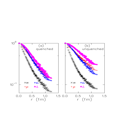
FIG. 6.: (a) Density-density correlators, $C({\bf r})$, for the pion, the rho, the nucleon and the $\Delta^{+}$ at $\kappa=0.154$ vs $|{\bf r}|$. (b) Same as (a) but with two dynamical quarks at $\kappa=0.157$. The dynamical results will be discussed in section V. We used the rho mass to set the scale in both the quenched and the unquenched theory. Errors bars are omitted for clarity.

Any asymmetry with respect to the spin axis $z$ is best seen by comparing the correlator $C({\bf r})$ for ${\bf r}=(x,y,0)$ and $(x,0,z)$, i.e. in a plane perpendicular to the spin axis and a plane containing it. The resulting contour plots are shown for $\kappa=0.154$ in Figs. 7 and 8 for the pion and the rho and in Figs. 9 and 10 for the nucleon and the $\Delta^{+}$. The cigar shape is clearly visible in the case of the rho, whereas the pion and the nucleon look spherical (up to small lattice distortions) as expected since their spectroscopic quadrupole is zero.

A small asymmetry appears for the $\Delta^{+}$, but it is not statistically significant. This is true for all the $\Delta^{+}$ spin projections. In Fig. 10 we select the unphysical state obtained using interpolating field $J_{3}$ because it should show maximal deformation. In the case of the $\Delta$, quenching removes only part of the pion cloud, contrary to the case of the rho where it is removed completely. Still, our negative finding does not rule out a deformation of the $\Delta$ induced by pions. It may be that the asymmetry only shows up when the quark mass is further decreased so that the pion has a mass close to its physical value, although we do not observe a statistically significant increase in the deformation as we go from quenched quarks of naive quark mass $m_{q}\sim 300$ MeV to $m_{q}\sim 90$ MeV. It could also be that the asymmetry is enhanced and only becomes visible in full QCD, with a complete pion cloud made of light enough pions. This issue is addressed in the next section.

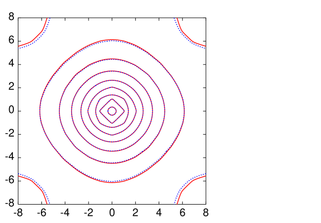
FIG. 7.: Contour plot of the pion correlator, $C({\bf r})$, at $\kappa=0.153$, when $r$ lies in the $xz$-plane (solid lines) or in the $xy$-plane (dashed lines) of size $16^{2}$.

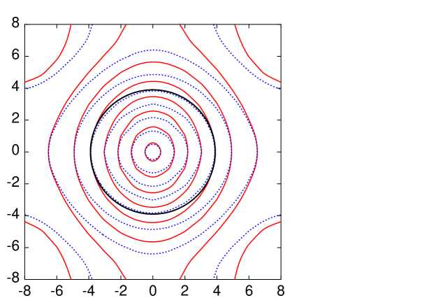
FIG. 8.: Same as Fig. 7 but for the rho for $J_{z}=0$. We have included a circle to guide the eye.

A more quantitative determination of meson deformations can be obtained by computing the second moments of the quark separation ${\bf r}$ along the three axes. Fig. 11 shows the second moments along the spin-axis, $\langle z^{2}\rangle$, and the average of the moments along the two transverse axes, $\langle(x^{2}+y^{2})/2\rangle$, plotted versus the pion mass squared. Here we use the rho mass to convert to physical units in order to be able to compare with the corresponding unequenched results.

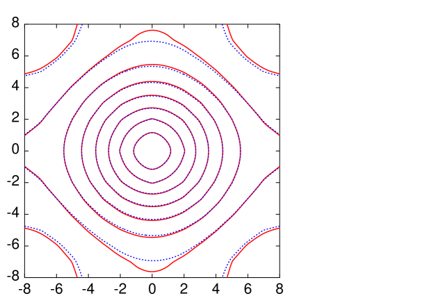
FIG. 9.: Same as Fig. 7 but for the nucleon.

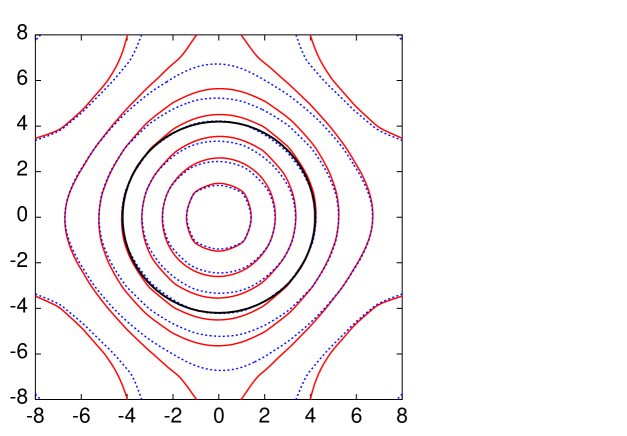
FIG. 10.: Same as Fig. 8 but for the $\Delta^{+}$. The interpolating field is $J_{3}$.

The spin-0 state of the rho shows an elongation along the spin-axis, which increases as the quark mass is decreased. As already mentioned, since this is a quenched calculation, this deformation is not due to the pion cloud. Therefore the situation may change if dynamical quarks are included. This is studied in Section V.

From the second moments we can obtain the charge root mean square (rms) radius of the mesons defined in the quark model by

$$<r^{2}_{\rm ch}> = \sum_{q}e_{q}\langle({\bf r}_{q}-{\bf R})^{2}\rangle$$ (25)

$$= \frac{\sum_{q}e_{q}\int d^{3}r\>({\bf r}/2)^{2}\>C({\bf r})}{\int d^{3}r\>C({\bf r})}$$ (26)

where ${\bf R}$ is the coordinate of the center of mass and $e_{q}$ is the electric charge of the quarks. In the chiral (quenched) limit we estimate for the pion $\sqrt{r^{2}_{\pi}}\sim 0.35$ fm using the rho mass to set the scale and 0.42 fm using the string tension [18] to be compared with the experimental value of 0.53 fm [21]. For the rho, using the rho mass and the string tension we find respectively $\sqrt{r^{2}_{\rho}}\sim 0.37$ fm and 0.44 fm. The ratio $\sqrt{r^{2}_{\rho}/r^{2}_{\pi}}\sim 1.06$ from the lattice data is somewhat small compared to the value 1.15, obtained from the experimental value 0.53 fm for the pion [21] and $0.61$ fm  for the rho [22] calculated in a Dyson-Schwinger equation approach using $f_{\pi}=93$ MeV. This discrepancy between the experimental and lattice results may be due to two reasons: 1) we are using the quenched theory where the pion cloud is eliminated and 2) we are far from the chiral limit and making a linear extrapolation in $m_{\pi}^{2}$ may be problematic, especially since chiral loops give a logarithmically divergent contribution to the pion and proton charge radii [23]. Lighter quark masses will be required to check the chiral extrapolation. In section V we will examine the effects of unquenching.

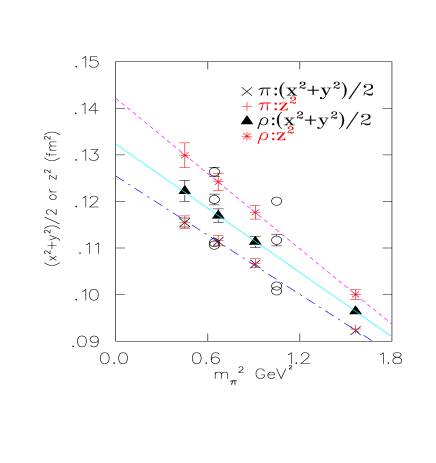
FIG. 11.: $\langle z^{2}\rangle$ and $\langle(x^{2}+y^{2})/2\rangle$ versus the pion mass squared in physical units. The lines are linear fits to the quenched data. The pion (dash-dotted line) is spherical. It is smaller than the rho, whose transverse size with respect to the spin axis (solid line) is smaller than its longitudinal size (dashed line). The rho (in the spin-0 projection) is shown to be cigar shaped, particularly in the chiral limit. The circles show full QCD results, discussed in section V.

A similar comparison of $\langle z^{2}\rangle$ with $\langle(x^{2}+y^{2})/2\rangle$ for the $\Delta^{+}$, using as interpolating field $J_{3}$ defined in Eq. 5, gives $\langle z^{2}\rangle>\langle(x^{2}+y^{2})/2\rangle$ (the reverse is true for the states with spin projection $\pm 3/2$), giving suspicion of a deformation. However, statistical errors are larger than the signal, so that we cannot claim to see any significant deformation.

B Three-density correlation functions

We have analysed 30 configurations at $\kappa=0.15$ and $\kappa=0.154$. Since we now have to consider two relative distances the calculation of the three-density correlations is more demanding even using FFT. As explained in section II we only compute the diagram with density insertions on different quark lines. However, we can check the quality of this approximation by integrating our three-density correlation over one relative distance, and comparing the result with the two-density correlation studied in the last subsection. If the three-density correlation contains complete information, both expressions should agree as per Eq. 19.

This comparison is performed in Fig. 12 for the nucleon, for two quark masses. Although the three-density correlation, as expected, is subject to larger finite-size effects visible for large quark separation, both methods give virtually identical results, indicating that we captured the dominant contribution to the three-density correlation. A similar conclusion holds for the $\Delta$.

In any case, the usefulness of three-density correlators is to supplement two-density correlators and expose more detailed structure: single-particle observables, such as the quadrupole moment, can be extracted directly from the two-density correlators.

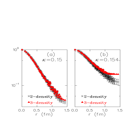
FIG. 12.: Single particle density for the nucleon (a) for $\kappa=0.15$ and (b) for $\kappa=0.154$.

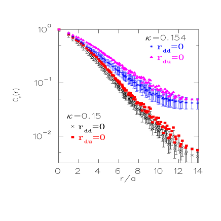
FIG. 13.: $u$- and $d$- quark spatial distributions in the neutron for $\kappa=0.15$ and $\kappa=0.154$. The errors bars for the $r_{du}=0$ case are comparable to those for the $r_{dd}=0$ case and are omitted for clarity.

The spatial $u$- and $d$- quark distributions in the nucleon can be investigated by fixing the relative position of the other two quarks. We note that, since we are using degenerate $u-$ and $d-$ quarks, only the electric charge differentiates the proton from the neutron. In Fig. 13 we show the spatial distributions of the $u$ and $d$ quark in the neutron, when the relative distance between the other two quarks is fixed to zero. For both quark masses considered, the $d$-quark spatial distribution is slightly broader than that of the $u$-quark. Since the total charge of the two $d$-quarks is -2/3 and that of the $u$-quark +2/3, the broader $d$-quark spatial distribution indicates that the charge root mean square radius of the neutron is negative. For the $\Delta^{+}$ the two distributions are the same. The charge radius squared can be evaluated using

$$\langle r^{2}_{\rm ch}\rangle=\frac{\int d^{3}{\bf r}_{1}\int d^{3}{\bf r}_{2}\sum_{q=1}^{3}e_{q}{\bf r}_{q}^{2}({\bf r}_{1},{\bf r}_{2})\>\>C({\bf r}_{1},{\bf r}_{2})}{\int d^{3}{\bf r}_{1}\int d^{3}{\bf r}_{2}\>\>C({\bf r}_{1},{\bf r}_{2})}$$ (27)

where ${\bf r}_{q}^{2}({\bf r}_{1},{\bf r}_{2})$ is the distance of each quark to the center of mass, in terms of the relative distances ${\bf r}_{1}$ and ${\bf r}_{2}$. Estimating this integral by a discrete lattice sum we obtain for the proton charge rms $(r_{p}/a)^{2}=20\pm 3.5$ or $\sqrt{r_{p}^{2}}\sim 0.45\pm 0.04$ fm at $\kappa=0.15$ and $(r_{p}/a)^{2}=27\pm 5.5$ or $\sqrt{r_{p}^{2}}\sim 0.52\pm 0.06$ fm at $\kappa=0.154$. If we extrapolate these two values linearly in $m_{\pi}^{2}$ to the chiral limit we find $\sim 0.59(4)$ fm, compared to the experimental value $0.81$ fm. Again we have used $a^{-1}=1.94$ GeV as determined from the string tension to convert to physical units. Using the nucleon mass in the chiral limit to set the scale gives $a^{-1}=1.88(7)$ GeV, very close to the value obtained from the string tension. If instead we would use the rho mass to set the scale, then $a^{-1}\approx 2.3$ GeV which gives for the proton, in the chiral limit, a smaller value equal to $\sqrt{r_{p}^{2}}\sim 0.50(4)$ fm. It has been pointed out that chiral logs can affect the chiral extrapolation of the radii and increase their value [23]. To check whether the chiral logs will produce larger values closer to the experimental result, additional $\kappa$ values closer to the chiral limit will be needed. The neutron charge radius square $r_{n}^{2}$ comes out negative for both values of $\kappa$ as expected. We obtain $r_{n}^{2}/r_{p}^{2}\sim-0.25\pm 0.08$ and $-0.29\pm 0.12$ at $\kappa=0.15$ and $\kappa=0.154$ respectively. These values are consistent with the experimental value of $-0.146$ albeit with large errors. Computing as a check the same quantity for the $\Delta^{+}$, we obtain zero within error bars, in agreement with our earlier observation that the $d$- and $u$- quark spatial distributions in the $\Delta^{+}$ are the same.

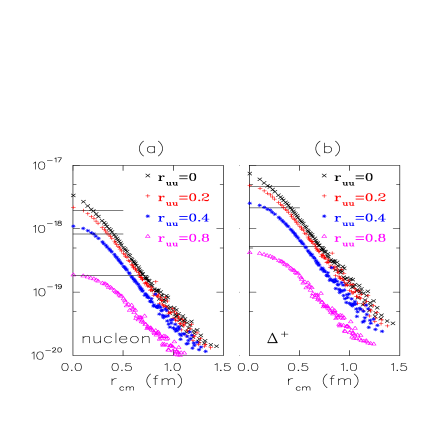
FIG. 14.: $d$-quark spatial distribution with respect to the center of mass of the two $u$-quarks, for different $u-u$ separations (a) in the nucleon spin +1/2 projection and (b) in the $\Delta^{+}$ spin +3/2 projection ($\kappa=0.15$). The straight lines mark the value of the wave function when $r_{uu}=0$ and the $u-d$ quark separation is 0.2, 0.4 and 0.8 fm, to be compared with $r_{cm}=0$ and $r_{uu}=0.2,0.4$ and 0.8 fm respectively.

Instead of fixing the relative distance between the two $u$-quarks in the proton or $\Delta^{+}$ to zero, we can fix it to various non-zero values. In Fig. 14 we fix the $u-u$ separation, $r_{uu}$, (between 0 and $8a$ along a principal lattice axis), and show the distribution of distances $r_{cm}$ between the $d$-quark and the $u-u$ center of mass. Detailed information about nucleon structure is contained in this figure.

In particular, let us compare configurations $(uu)-d$ where the two $u$-quarks at at the same place i.e. $r_{uu}=0$, and $u-d-u$ where the $d$-quark lies in the middle of the two $u$-quarks, i.e. $r_{cm}=0$ where $r_{cm}$ is the distance from the $d$-quark to the center of mass of the two $u$-quarks. As we will see in the next paragraph, effective models (both Y- and $\Delta$-Ansätze) predict equality of the wave functions among these two configurations provided they have the same total size (ie. $r_{cm}$ in $(uu)-d$ equal to $r_{uu}$ in $u-d-u$). Inequality reveals a finer structure than captured by effective models. It is clear from Fig. 14 that the top horizontal line ($(uu)-d$ with $r_{cm}=0.2$ fm) falls below the + sign at $r_{cm}=0$ ($u-d-u$ with $r_{uu}=0.2$ fm), indicating a relative suppression of the $(uu)-d$ configuration, i.e. a mutual $u-u$ repulsion. The same effect is visible for a larger configuration of size 0.4 fm (second horizontal line), but goes away or even gets inverted for yet larger configurations. Somewhat surprisingly, this $u-u$ repulsion at close range seems weaker in the $\Delta^{+}$ where the two $u$-quarks are in the same spin state (Fig. 14(b)) than in the nucleon where they can be in opposite spin states (Fig. 14(a)). This example, where a quantitative refinement could be obtained straightforwardly by considering lighter quarks on a larger lattice, serves to illustrate the wealth of information contained in three-density correlators.

Having, in the non-relativistic limit, the wave function of a baryon it is interesting to ask whether we can deduce the potential which would yield this wavefunction. The relevant potential will of course depend on the two relative distances between the quarks. The issue is whether we can further reduce the degrees of freedom to effectively write the confining potential in terms of one distance only. Two such proposals exist in the literature, which make different predictions for the linear rise of the baryonic potential. $(i)$ The so called Y-Ansatz can be derived by a strong coupling argument [24]: the baryon potential grows in proportion to the minimal length of gluonic string necessary to join together the three static quarks. The three strings join at the Steiner point. $(ii)$ The so called $\Delta$-Ansatz is derived from a center vortex picture of confinement [11]. The baryonic potential is simply a sum of two-body $q\bar{q}$ potentials and grows like $\frac{\sigma}{2}(r_{12}+r_{23}+r_{31})$, where $\sigma$ is the $q\bar{q}$ string tension and $r_{ij}$ the $q_{i}-q_{j}$ distance. The difference between these two Ansätze depends on the geometry of the three quark system. For instance it vanishes when the three quarks are aligned, since then the Steiner point which minimizes the length of flux tube joining the three quarks coincides with the position of the middle quark. Unfortunately this difference never exceeds $\sim 15$%, so that very accurate results at large quark separations $\sim 1$ fermi are needed to ascertain which model, if any, is correct. In a recent lattice calculation of the baryonic potential it was shown that the $\Delta$-Ansatz is favoured for distances up to 0.8 fm [25]. Although this finding is in agreement with the results of [26], a different analysis of similar lattice results has led others [27] to the conclusion that the Y-Ansatz is preferred. This issue is currently under further study both on the lattice [28] and phenomenologically [29].

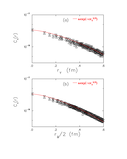
FIG. 15.: Nucleon wave function (a) versus half the $\Delta$-distance and (b) versus the Y-distance.

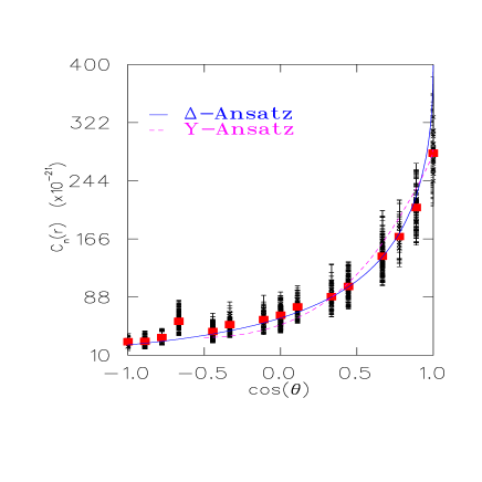
FIG. 16.: Theta dependence of the nucleon wave function when the two relative distances are fixed to $0.6\pm 0.001$ fm. The filled squares are the central values of the wave function. The solid line is the fit using the $\Delta$-Ansatz for the angular dependence and the dashed line is the corresponding fit using the $Y-$ Ansatz. Note that for $\cos{(\theta)}<-0.5$ the $Y$-Ansatz coincides with the $\Delta$-Ansatz.

To examine whether our wave function results favour one of these two Ansätze, we plot them as a function of $r_{Y}$ (Fig. 15(a)) and of $r_{\Delta}$ (Fig. 15(b)), where $r_{Y}$ is the minimal total length of the flux strings and $r_{\Delta}=1/2(r_{12}+r_{23}+r_{31})$. The scatter of the data is visibly smaller when plotted as a function of $r_{\Delta}$, indicating that $r_{\Delta}$ is a better effective variable than $r_{Y}$. Furthermore, consider the solution to the non-relativistic Schrödinger equation with potential $V_{Y}\propto r_{Y}$ or $V_{\Delta}\propto r_{\Delta}$. It is an Airy function which asympotically decays as $\exp(-cr^{3/2})$. Fits of the wave function of the nucleon to this asymptotic form are shown in Fig. 15. The fit using the $r_{\Delta}$ as the relevant distance yields a $\chi^{2}/{\rm d.o.f}=0.4$ whereas using $r_{Y}$ one gets $\chi^{2}/{\rm d.o.f}=1.0$. Therefore both Ansätze provide a surprisingly good description of the wave function, with a preference for the $\Delta$-Ansatz.

As a more stringent test, we fix the relative distances $|{\bf r}_{1}|=|{\bf r}_{2}|$ between the $d$ and the two $u$ quarks, and study the wave function as a function of the $\hat{udu}$ angle, $\cos(\theta)={\bf r}_{1}.{\bf r}_{2}/|{\bf r}_{1}||{\bf r}_{2}|$, that the relative distances make. Both for the $\Delta$- and $Y-$ Ansätze the wave function should only depend on this angle but with a different functional dependence. In Fig. 16 we show the wave function for the nucleon versus the cosine of the angle. Again the $\Delta$-Ansatz provides a better description of the data.

V Density-density correlators with two dynamical quarks

As we noted in the previous section, if the pion cloud is responsible for hadron deformation, then the quenched and unquenched results may differ significantly. To investigate the importance of dynamical quarks, we used the SESAM [13] configurations with two dynamical degenerate quark species at $\beta=5.6$ on a lattice of size $16^{3}\times 32$. The lattice spacing determined from the rho mass in the chiral limit is $a^{-1}=2.3$ GeV [13] which is same as for the quenched theory at $\beta=6.0$ and therefore the physical volume is the same as in our quenched calculation. We use this determination of the lattice spacing, which is applicable in both the quenched and the unquenched theory, to compare results among both. We have analysed 150 configurations at $\kappa=0.156$ and 200 at $\kappa=0.157$. The ratio of the pion mass to rho mass is 0.83 at $\kappa=0.156$ and 0.76 at $\kappa=0.157$. These values are close to the quenched mass ratios measured at $\kappa=0.153$ (0.84) and $\kappa=0.154$ (0.78) respectively, allowing us to make pairwise quenched-unquenched comparisons.

In Fig. 6(b) we plot the two-density correlators for the four hadrons for light sea quarks ($\kappa=0.157$). Comparing with the quenched results ($\kappa=0.154$), one sees that the pion size remains the same, but that the rho, nucleon and $\Delta^{+}$ sizes increase. The $\Delta^{+}$ is now clearly larger than the rho and the rho correlator decays more slowly than the nucleon. This slower decay is also visible in the quenched case for $\kappa=0.154$ and $0.155$ but not for the smaller values of $\kappa$. The invariance of the pion size can be also seen in Fig. 11 which shows the second moments. This result is consistent with calculations in the Dyson-Schwinger framework which concluded that the pion cloud, consisting of physical pions, contributes only 15% to the root mean square radius of the pion [30]. In our simulations the effect is expected to be even smaller since the pion mass is larger than 600 MeV. On the other hand, Fig. 11 shows that unquenching increases the rho size and therefore the ratio of the rho charge radius to the pion’s approaches the experimental value. This ratio is expected to be more reliable than the individual moments since lattice artifacts partly cancel out.

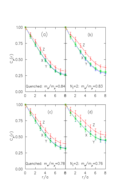
FIG. 17.: Asymmetry for the rho wave function (a) in the quenched approximation at $\kappa=0.153$ and (c) at $\kappa=0.154$ and (b) for two dynamical quarks at $\kappa=0.156$ and (d) $\kappa=0.157$ .

From Fig. 17 we compare the quenched and unquenched asymmetry in the rho for comparable ratios $m_{\pi}/m_{\rho}$. The main observation is that the asymmetry in the rho grows in full QCD. This is clearly seen in the (a)-(b) comparison, i.e. for the heavier dynamical quarks. For the lighter quarks (c)-(d), this growth in the asymmetry is still there but the effect seems less pronounced. On the other hand, finite-size effects are more important. Disentangling the two would require larger lattices.

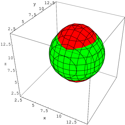
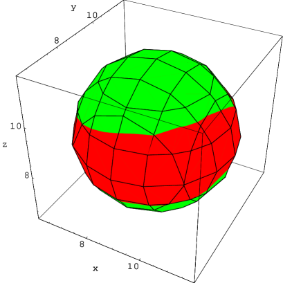
FIG. 18.: Three-dimensional contour plot of the correlator (black): upper for the rho state with 0 spin projection (cigar shape) and lower for the $\Delta^{+}$ state with +3/2 (slightly oblate) spin projection for two dynamical quarks at $\kappa=0.156$. Values of the correlator (0.5 for the rho, 0.8 for the $\Delta^{+}$) were chosen to show large distances but avoid finite-size effects. We have included for comparison the contour of a sphere (grey).

The same analysis for the $\Delta^{+}$ gives no definite results regarding the deformation. Whereas in all channels we do observe a deformation obeying the sign relations obtained in Section II with the Wigner-Eckart theorem, the deformation remains small with large statistical errors. However it is interesting to look at a three-dimensional contour plot for the $\Delta^{+}$ in the $+3/2$ spin state and compare it to the rho 0-spin state. In Fig. 18 we show these contour plots for the heavier sea quarks that we analyzed. The elongation in the rho is clearly visible whereas the $\Delta^{+}$ appears to be squeezed. Note that squeezing in this channel means that the unphysical channel using an interpolating field a $J_{3}$ in Eq. 5 is elongated. The statistical uncertainties are larger for the lighter sea quark but the trend for the deformation remains the same. The overall conclusion is that unquenching seems to increase the deformation for the $\rho$ and the $\Delta$, which would imply that the pion cloud contributes to the deformation of these hadrons. However more statistics, a bigger lattice and lighter quark masses will be needed to consolidate this observation.

VI Conclusions

Two-density correlators for mesons and baryons are shown to contain rich information on their structure. For the baryons these correlators reduce to the one-particle density in the non-relativistic limit.

The overall quark mass dependence of the correlators for the pion, the rho, the nucleon and the $\Delta^{+}$ is found to be rather weak. The rho correlator shows the strongest dependence on the quark mass, and the nucleon and the $\Delta$ the weakest. For the quark masses that we have studied in this work unquenching has the strongest effect on hadron sizes for the rho and the $\Delta$, and the weakest for the pion and the nucleon. In the quenched approximation we find that the rho state with 0-spin projection is prolate, whereas for the $\Delta^{+}$ no statistically significant deformation is seen. Since for the rho there are no virtual pions from backward moving quarks in the quenched approximation, the rho deformation is a dynamic property of quarks forming a vector particle. Adding sea quarks while keeping the pion to rho mass ratio constant, we observed an increase in the rho deformation, and a slight oblate deformation of the $\Delta^{+}$ $+3/2$ spin state. The pion cloud may be responsible for this effect. As already pointed out, lighter sea quark masses together with a larger lattice to well contain the hadrons will be needed in order to study further the role of the pion cloud.

Three-density correlators for baryons, although computed neglecting insertions on the same quark line, are shown to reproduce the two-density correlators when integrated over one relative coordinate. Therefore one expects the contribution of the neglected diagram with two insertions on the same quark line to be small. With the three-density correlators baryonic structure can be explored in more detail. In the neutron we clearly detect a broader $d$-quark spatial distribution compared to that of the $u$-quark. This accounts for the negative charge square radius of the neutron observed experimentally. By comparing the $u$- and $d$- spatial distributions in the proton and in the $\Delta^{+}$ we observe that there is a preference for the two $u$-quarks to be at 180⁰ rather than at the same place. More statistics are needed to consolidate the trend observed here.

Information on the baryonic potential can be extracted from fits to the three-density correlators of the nucleon. By performing a fit to the radial and angular dependence we find that the baryonic wave functions are better described by a confining potential which is the sum of two-body potentials known as the $\Delta$-Ansatz, at least for relative distances of $\sim 1$ fm that we can probe in this work.

Acknowledgements: We thank C. N. Papanicolas for encouraging us to look into the issue of deformation and for discussions. The $SU(3)$ $16^{3}\times 32$ quenched lattice configurations were obtained from the Gauge Connection archive [17]. We thank the SESAM collaboration for giving us access to their dynamical lattice configurations.

REFERENCES

- [1] S. Aoki et al. [CP-PACS Collaboration], Phys. Rev. Lett. 84 (2000) 238 [arXiv:hep-lat/9904012]; K. C. Bowler et al. [UKQCD Collaboration], Phys. Rev. D 62 (2000) 054506 [arXiv:hep-lat/9910022].
- [2] C. J. Morningstar and M. Peardon, Phys. Rev. D 60 (1999) 034509 [arXiv:hep-lat/9901004].
- [3] B. Velikson and D. Weingarten, Nucl. Phys. B 249 (1985) 433; S. Gottlieb, in Advances in Lattice Gauge Theory, World Scientific, 1985, p. 105.
- [4] M. W. Hecht and T. A. DeGrand, Phys. Rev. D 46 (1992) 2155.
- [5] R. Gupta, D. Daniel and J. Grandy, Phys. Rev. D 48 (1993) 3330.
- [6] W. Wilcox, K. F. Liu, Phys. Rev. D 34 (1986) 3882; S. Huang, J. W. Negele and J. Polonyi, Nucl. Phys. B 307 (1988) 669; M. C. Chu, M. Lissia and J. W. Negele, Nucl. Phys. B 360 (1991) 31.
- [7] N. Isgur, G. Karl and R. Koniuk, Phys. Rev. D 25 (1982) 2394; S. Capstick and G. Karl, Phys. Rev. D 41 (1990) 2767.
- [8] A. J. Buchmann and E. M. Henley, Phys. Rev. C 63 (2001) 015202 [arXiv:hep-ph/0101027].
- [9] C. Mertz et al., Phys. Rev. Lett. 86 (2001) 2963 [arXiv:nucl-ex/9902012].
- [10] D. B. Leinweber, T. Draper and R. M. Woloshyn, Phys. Rev. D 48 (1993) 2230 [arXiv:hep-lat/9212016].
- [11] J. M. Cornwall, Phys. Rev. D 54 (1996) 6527 [arXiv:hep-th/9605116].
- [12] T. D. Cohen and D. B. Leinweber, Comments Nucl. Part. Phys. 21 (1993) 137 [arXiv:hep-ph/9212225].
- [13] N. Eicker et al. [SESAM collaboration], Phys. Rev. D 59 (1999) 014509 [arXiv:hep-lat/9806027].
- [14] K. B. Teo and J. W. Negele, Nucl. Phys. Proc. Suppl. 34 (1994) 390; J. W. Negele, arXiv:hep-lat/0007026.
- [15] M. Burkardt, J. M. Grandy and J. W. Negele, Annals Phys. 238 (1995) 441 [arXiv:hep-lat/9406009].
- [16] W. Wilcox, Phys. Lett. B 289 (1992) 411 [arXiv:hep-lat/9207014]; arXiv:hep-lat/9606019.
- [17] http://qcd.nersc.gov
- [18] G. S. Bali, C. Schlichter and K. Schilling, Phys. Rev. D 51 (1995) 5165 [arXiv:hep-lat/9409005].
- [19] Y. Iwasaki et al., Phys. Rev. D 53 (1996) 6443.
- [20] T. Bhattacharya, R. Gupta, G. Kilcup and S. Sharpe, Phys. Rev. D 53(1996) 6486.
- [21] S. R. Amendolia et al. [NA7 Collaboration], Nucl. Phys. B 277 (1986) 168.
- [22] F. T. Hawes and M. A. Pichowsky, Phys. Rev. C 59 (1999) 1743 [arXiv:nucl-th/9806025].
- [23] M. A. Beg and A. Zepeda, Phys. Rev. D 6 (1972) 2912; D. B. Leinweber and T. D. Cohen, Phys. Rev. D 47 (1993) 2147 [arXiv:hep-lat/9211058].
- [24] J. Carlson, J. Kogut and V. R. Pandharipande, Phys. Rev. D 27 (1983) 233; Phys. Rev. D 28 (1983) 2807.
- [25] C. Alexandrou, P. de Forcrand and A. Tsapalis, Phys. Rev. D 65 (2002) 054503 [arXiv:hep-lat/0107006]; Nucl. Phys. Proc. Suppl. 106 (2002) 403 [arXiv:hep-lat/0110115]; Nucl. Phys. Proc. Suppl. 109 (2002) 153 [arXiv:nucl-th/0111046].
- [26] G. S. Bali, Phys. Rept. 343 (2001) 1 [arXiv:hep-ph/0001312].
- [27] T. T. Takahashi, H. Matsufuru, Y. Nemoto and H. Suganuma, Phys. Rev. Lett. 86 (2001) 18 [arXiv:hep-lat/0006005]; arXiv:hep-lat/0107008; arXiv:hep-lat/0204011.
- [28] C. Alexandrou, Ph. de Forcrand and O. Jahn, arXiv:hep-lat/0209062 and in writing.
- [29] D. S. Kuzmenko and Y. A. Simonov, Phys. Lett. B 494 (2000) 81 [arXiv:hep-ph/0006192]; Phys. Atom. Nucl. 64 (2001) 107 [Yad. Fiz. 64 (2001) 110] [arXiv:hep-ph/0010114].
- [30] R. Alkofer, A. Bender and C. D. Roberts, Int. J. Mod. Phys. A 10 (1995) 3319 [arXiv:hep-ph/9312243].