Chiral Measurements in Quenched
Lattice QCD with Fixed Point
Fermions

Inauguraldissertation
der Philosophisch-naturwissenschaftlichen Fakultät
der Universität Bern

vorgelegt von

Thomas Jörg

von Winterthur (ZH)

Leiter der Arbeit: Prof. Dr. P. Hasenfratz Institut für theoretische Physik Universität Bern

Abstract

The low-energy sector of Quantum Chromodynamics (QCD), which is dominated by a very strong interaction between the quarks and the gluons, is an excellent example of how an analytical and a numerical approach can work together and thereby mutually increase their predictive power.

Chiral Perturbation Theory ($\chi$PT) offers a systematic method to predict analytical dependencies of different physical quantities in the low-energy region of QCD. It is, however, an effective theory which is based on the – generally accepted – assumption that chiral symmetry is spontaneously broken in massless QCD and relies on data from other sources to fix the low-energy constants in its Lagrangian.

Lattice QCD, which is the only non-perturbative regularization of QCD known at the moment, is heavily based on numerical methods. It offers the possibility to calculate quantities in QCD from first principles. But it has shown to be a very delicate problem to incorporate chiral symmetry on the lattice. A fact which lead to many technical and fundamental problems. The recently rediscovered Ginsparg-Wilson relation is equivalent to chiral symmetry on the lattice and with this a long standing problem in Lattice QCD was solved. Having chiral fermions on the lattice leads to a much better control in calculations where chiral symmetry is important and allows to test the assumption of the spontaneous breakdown of chiral symmetry in QCD in a cleaner way than with traditional lattice fermions.

Fixed Point (FP) Dirac operators are designed to solve another big problem in lattice simulations, the discretization errors introduced by putting a theory on the lattice. Because FP Dirac operators have been shown to satisfy the Ginsparg-Wilson relation, they combine two important virtues one can wish a lattice Dirac operator to have.

In this work we construct a parametrization of a FP Dirac operator and apply it in quenched Lattice QCD. The symmetry requirements for a lattice Dirac operator are discussed and an efficient way to make a practical construction of general lattice Dirac operators is provided. We use such a general lattice Dirac operator to approximately solve the Renormalization Group equation that defines the FP Dirac operator in an iterative procedure. We discuss the properties of this parametrization and show that its breaking of chiral symmetry is much reduced compared to the most frequently used lattice Dirac operator, the Wilson Dirac operator. Furthermore, we discuss the overlap construction with the parametrized FP Dirac operator. With this construction the remaining chiral symmetry breaking of the parametrization can be reduced systematically to a desired level. We show that the locality of the overlap construction with our Dirac operator is improved with respect to the common overlap construction with the Wilson Dirac operator. Using the overlap construction with the parametrized FP Dirac operator we perform several test calculations, where a precise chiral formulation of the lattice Dirac operator is needed or desirable. Using the Atiyah-Singer index theorem, which is a consequence of chiral symmetry, we calculate the quenched topological susceptibility. The results are consistent with other recent determinations, but they are not accurate enough to make a controlled continuum extrapolation. We also confirm recent results about the local chirality of near-zero modes of the Dirac operator. Finally, we determine the low-energy constant $\Sigma$ of quenched Chiral Perturbation Theory, which in full QCD with $3$ light flavors would correspond to $-\langle\bar{\psi}\psi\rangle$, the order parameter of spontaneous symmetry breaking.

Chapter 1 Introduction

Over the last 30 years Quantum Chromodynamics (QCD) has been very successful in explaining many phenomena of the strong interactions. Using standard perturbation theory, which was developed in the framework of Quantum Electrodynamics (QED), processes involving high energies can be studied in a systematic manner. However, at energies below $1\,{\rm GeV}$ the strong coupling constant $\alpha_{s}$ gets of ${\cal O}(1)$ such that standard perturbative methods fail – a fact which has many consequences. Not only that the interesting physics of particles like protons and neutrons, out of which nuclear matter in our surroundings consists, is governed by the non-perturbative properties of QCD, but also that confinement of quarks, a profound property of QCD, makes that in experiments always bound states of quarks and gluons – the so called hadrons – are observed. This implies that in order to compare the perturbative calculations with experiments one typically needs information about the low-energy behaviour of QCD, e.g. in form of hadronic matrix elements.

Certain non-perturbative problems of QCD can be treated analytically using an effective theory for the Goldstone bosons degrees of freedom. This approach assumes that chiral symmetry is spontaneously broken [1, 2, 3, 4, 5]. This spontaneous breaking of chiral symmetry leads to the appearance of massless excitations – the Goldstone bosons – if the mass of the quarks is set to $0$. In nature the masses of the lightest quarks are not $0$, but a few ${\rm MeV}$ for the up and down quark and roughly $120\,{\rm MeV}$ for the strange quark. Hence, chiral symmetry is broken also explicitly by the quark mass terms. It however shows that these masses are still small enough compared to the intrinsic scale of QCD, $\Lambda_{\rm QCD}$, that the effect of the spontaneous breakdown of chiral symmetry dominates the low-energy structure. Chiral Perturbation Theory ($\chi$PT), which is a systematic expansion in the quark masses and momenta of the light quarks, has been very successful in predicting many of the low-energy properties of QCD, such as e.g. quark mass ratios, scattering lengths and, in general, properties of the Goldstone bosons ($\pi$,K,$\bar{\rm K}$,$\eta$). However, being an effective theory the predictions of $\chi$PT rely on accurate determinations of low-energy constants, which have to be extracted from various experimental data. For certain of these constants this shows to be rather difficult, if it is possible at all. Furthermore, $\chi$PT works well only within a limited range of energies, which moreover may vary from process to process under consideration.

The lattice approach to QCD is a radically different way to have access to the low-energy structure of QCD, as it gives a completely non-perturbative definition of QCD. The idea, which has been proposed by Wilson in 1974 [7], is to discretize the QCD action by replacing the continuum space-time by a discrete four-dimensional lattice with a finite lattice spacing $a$. It is the only definition of QCD beyond the perturbative level known at the moment and it provides, at least in principle, a tool to study QCD from first principles. Calculations in Lattice QCD involve the numerical evaluation of the path integral defining the discretized QCD action by stochastic sampling (Monte Carlo) techniques. The way from the point where one writes down the discretized QCD action to the point where one can extract accurate physical data which is relevant for QCD phenomenology has, however, shown to be more tedious and longer than expected in the early 1980’s. In order to understand this we focus on two fundamental problems in lattice QCD: Chiral symmetry and discretization errors.

In defining a disretized version of the gluonic as well as the fermionic part of the Lattice QCD action one has, in fact, an infinite choice of discretizations. The discretizations which are the most popular are the Wilson gauge action and the Wilson Dirac operator. These actions define the simplest way how the theory can be discretized with the right continuum limit $a\to 0$ and essentially without destroying the subtle structure of the anomalies of QCD. The Wilson Dirac operator, however, in order to avoid the problem of species doubling — an effect we will discuss below — introduces a term that breaks chiral symmetry explicitly. This so-called Wilson term is an irrelevant operator and therefore chiral symmetry is restored in the continuum limit, but the costs are high. Due to the breaking of chiral symmetry the Wilson operator introduces errors of ${\cal O}(a)$ into the lattice discretization and, furthermore, the quark mass gets additively renormalized, operators in different chiral representations get mixed and additional renormalization factors have to be calculated. All these problems are essentially of technical nature, but they make the extraction of physical data at least very tedious, thereby hiding the underlying chiral structure of QCD. For chiral gauge theories like the electroweak sector of the Standard Model, however, the explicit breaking of chiral symmetry has so far precluded all attempts to achieve a realistic lattice formulation. Another approach to put fermions on the lattice, which is used very often in simulations, are the so-called staggered or Kogut-Susskind fermions [8]. They partially solve the problem of the species doubling by reducing the number of doublers from 16 to 4 and thereby also solve the problem of chiral symmetry breaking to a large extent by leaving a chiral ${\rm U}(1)$ subgroup invariant. However, they introduce a new headache: they break flavor symmetry, which makes the construction of hadron operators with the correct quantum numbers rather difficult. Even though staggered fermions have only ${\cal O}(a^{2})$ discretization errors, these errors can be large [9], making it necessary to go far to the continuum limit in order to get physical results that are not contaminated too heavily by the discretization.

In order to reduce lattice artifacts Symanzik has proposed the idea that one can add irrelevant higher order terms to the initial action such that the leading cut-off effects are cancelled [11, 12]. This idea is implemented in the Lüscher-Weisz action [13] and the Sheikholeslami-Wohlert (clover) Dirac operator [14]. Similarly, other improvement programmes were pursued, most prominently the non-perturbative clover improvement, which eliminates all the ${\cal O}(a)$ effects [15]. This programme has shown to be very successful in the determination of hadron masses, which show a very nice scaling behaviour, whereas for other quantities the ${\cal O}(a^{2})$ cut-off effects can still be large.

This brings us to the main topic of this work, the fixed point approach to QCD. Wilson’s Renormalization Group (RG) approach offers a radical way to treat the problem of lattice artifacts [16, 17, 18]. Using so-called quantum perfect actions one gets entirely rid of the lattice artifacts. Such actions are unfortunately very difficult to approximate and to really solve the defining RG equations is out of reach. Hasenfratz and Niedermayer have shown [19] that for asymptotically free field theories – like QCD – it is possible to define a so-called classically perfect or fixed point (FP) action that reproduces the properties of the corresponding classical theory without discretization errors. In fact, this corresponds to an on-shell Symanzik improvement at tree-level to all order in $a$. For asymptotically free theories, where the continuum limit corresponds to the limit where the coupling goes to $0$, such a FP action is expected to be a close approximation to the quantum perfect action even at non-zero coupling.

The FP Dirac operator $\operatorname{\textfrak{D}_{\rm FP}}$ does not only have reduced cut-off effects, but as pointed out by Hasenfratz in 1997, it satisfies the Ginsparg-Wilson (GW) relation [20]

$$\{\operatorname{\textfrak{D}},\gamma_{5}\} =\operatorname{\textfrak{D}}{\gamma_{5}}2R\operatorname{\textfrak{D}}\,,$$ (1.1)

or equivalently

$$\,\{\operatorname{\textfrak{D}}^{-1},\gamma_{5}\} =\gamma_{5}2R\,,$$ (1.2)

where $\operatorname{\textfrak{D}}$ is the lattice Dirac operator and $R$ is a local, hermitian operator which commutes with $\gamma_{5}$. The GW relation is equivalent to have chiral symmetry on the lattice, as Lüscher has shown in 1998 [21]. Hence, FP actions offer a solution to two of the fundamental problems – chiral symmetry and cut-off effects – which have been making the extraction of physical results from lattice simulations in QCD difficult over the last 20 years. Let us mention at this point that even though this work is concerned mainly with the chiral aspects of the FP approach, i.e. its application to very light quarks, the FP QCD action has also the potential to be used in lattice simulations with heavy quarks – especially the charm quark – because these simulations, which are performed at momentum scales near the cut-off, are particularly subject to distortions by the discretized action. The application of FP actions to this topic, however, remains unexplored also in this work.

There are other (approximate) solutions to the GW relation which are essentially focussed on the aspect of chiral symmetry, such as e.g. the approach of Gattringer, Hip and Lang to approximate a solution of the GW relation by a systematic expansion in operators built out of paths up to a certain length [22, 23, 24]. The most prominent examples are, however, the 5 dimensional domain-wall (DW) fermions [25, 26, 27] and the related overlap fermions [28, 29, 30], which are both based on a proposition made by Kaplan in 1992. For more informations on these approaches we refer to the recent reviews in [31, 32, 33] for the DW fermions and to [33] for the overlap fermions. Both constructions, in contrast to the FP Dirac operator, are defined in such a way that it is more or less straight forward to implement them in simulations, even though they are numerically very expensive. In fact, the costs of simulations with (approximately) chiral fermions in quenched QCD are roughly the same as full QCD simulations with Wilson fermions, i.e. that it is ${\cal O}(10)-{\cal O}(100)$ times more expensive than quenched simulations with Wilson fermions.

Most of the simulations with (approximately) chiral fermions and also the largest ones have been performed with DW fermions. Long standing problems, where chiral symmetry plays an essential rôle, have been tackled. Examples are the weak interaction matrix elements, such as those relevant for kaon physics, i.e. the $B$-parameter $B_{K}$, the $\Delta I=1/2$ rule and the parameter of direct CP violation $\epsilon^{\prime}/\epsilon$ [34, 35, 36]. The results of these very intricate calculations, however, are clearly a deception, as the sign of $\epsilon^{\prime}/\epsilon$ measured on the lattice is opposite to the experimental value and for the magnitude of relevant parameter of the $\Delta I=1/2$ rule the two large lattice simulations (RBC, CP–PACS) differ roughly by a factor of $2$ from each other. This raises the question where these problems come from. The answer is not definitively clear, but it has shown that it is rather difficult to have good control over the remaining breaking of chiral symmetry in the DW fermion approach, even though the linear extent of the fifth dimension $N_{s}$ can be used to extrapolate to the limit $N_{s}\to\infty$, where the DW fermions get exactly chiral. But there is evidence that the convergence is rather slow [32]. There are propositions how this problems can be solved [37, 38] and also the overlap fermion approach offers very good possibilities to control the remaining breaking of chiral symmetry. Future simulations will show whether the problems of the DW approach are really related to the remaining symmetry breaking or whether other possible explanations as e.g. discussed in [35, 9] are more relevant.

The definition of chiral fermions on the lattice has yielded the hope that finally chiral gauge theories can be formulated on the lattice and, indeed, the last years have seen a lot of progress in this area [39, 40, 41, 42, 21, 43, 44, 45, 46, 47, 48, 49, 50, 51, 52, 53, 54, 55, 56, 57, 58, 59, 60, 61, 62]. There remain, however, several open questions, like the relative weight factors between the topological sectors, the fate of CP symmetry and a related question about the definition of Majorana fermions [9, 63, 64]. Early hopes that a GW like approach might work for supersymmetry also did not realize either.

Before we embark upon a more detailed discussion of chiral symmetry in QCD and chiral fermions on the lattice — in particular fixed point fermions — let us give an outline of this work.

In Chapter 2 we discuss the structure of a general lattice Dirac operator that satisfies all the basic symmetry conditions, which are gauge symmetry, hermiticity condition, charge conjugation, hypercubic rotations and reflections. We give examples of terms that can occur in such a general operator, which are specific for our parametrization of the FP Dirac operator, and show how one can use them in a practical application.

The details of the parametrization of the FP Dirac operator are discussed in Chapter 3. The parametrization turns out to be quite difficult and a lot of effort has been put into this part of this work, because the results in the simulations clearly depend on the quality of the parametrization.

In Chapter 4 we give a summary of the properties of the parametrized FP Dirac operator. We mainly focus on the chiral properties, however, also scaling properties are discussed to a certain extent. The main source of data on scaling properties is the hadron spectroscopy study which is presented in the PhD thesis of Simon Hauswirth [65].

Chapter 5 explains Neuberger’s overlap formula and its application to the overlap construction with the parametrized FP Dirac operator. Furthermore, properties of this specific overlap operator are discussed. In particular, we show that our overlap construction is more local than the usual construction with the Wilson Dirac operator.

In Chapter 6 we present results for the quenched topological susceptibility and the local chirality of near-zero modes.

The determination of the low-energy constant $\Sigma$ of quenched Chiral Perturbation Theory, which in full QCD with 3 light flavors is equal to the order parameter of spontaneous chiral symmetry breaking $\langle\bar{\psi}\psi\rangle$, is given in Chapter 7.

Conclusions and prospects are given in Chapter 8.

Finally, this thesis covers only part of the work that has been done in collaboration with Simon Hauswirth, Kieran Holland, Peter Hasenfratz and Ferenc Niedermayer in an ongoing project, where the parametrized FP Dirac operator is tested and applied to various calculations in quenched QCD. Parts of it have already been published in [66, 67, 68, 69] and much more information can be found in [65].

1.1 Chiral Symmetry in QCD

In this section we give a short overview of various aspects and consequences of the symmetries of QCD. We will, however, not discuss interesting properties of QCD, such as asymptotic freedom, confinement and various other topics and refer the reader to one of the many books about QCD e.g. [70, 71]. We will keep the discussion in the framework of QCD, because the discussion of the same topics in quenched QCD is heavily loaded by various technicalities that rather hide the structure of chiral symmetry and its consequences. We will, however, mention the differences between the quenched approximation and real QCD there where it is needed and we will, in particular, point to the differences in those chapters where we measure quantities in quenched QCD.

Symmetries are a very important concept in physics since their presence always simplifies analysis and in certain cases allows one to obtain exact or semi-exact results. In QCD the presence of light quarks are the reason for an approximate symmetry and this allows one to extract a lot of consequences concerning the dynamics of the theory.

In Euclidean space, the Lagrangian of QCD with the gluon field strength tensor ${F}_{\mu\nu}$, the quark fields $\psi_{f}$, the Dirac operator ${\cal D}\!\!\!\!/$ and the gauge coupling $g$ reads

$${\cal L}_{QCD}=\frac{1}{4g^{2}}{F}^{a}_{\mu\nu}{F}^{a}_{\mu\nu}\ +\ \sum_{f=1}^{6}\bar{\psi}_{f}({\cal D}\!\!\!\!/+m_{f})\psi_{f}\ ,$$ (1.3)

where $m_{f}$ are the quark masses. The up, down, and strange quarks are relatively light, with masses $m_{u}\approx 3\ {\rm MeV},\ m_{d}\approx 6\ {\rm MeV}$, and $m_{s}\approx 120\ {\rm MeV}$. There is a clear gap between $m_{u,d}$, which are especially small, and the masses of the charm, bottom and top quark with $m_{c}\approx 1.25\,{\rm GeV}$, $m_{b}\approx 4.2\,{\rm GeV}$ and $m_{t}=174.3\pm 5.1\,{\rm GeV}$ [72]. It makes sense to consider the chiral limit when $N_{f}=2$ or $N_{f}=3$ quarks become massless and the other quark masses are sent to infinity. In this limit, the Lagrangian (1.3) is invariant under the transformations

$$\delta_{a}\psi =i\epsilon T_{a}\psi\,, \delta_{a}\bar{\psi} =-i\epsilon\bar{\psi}T_{a}\,,$$ (1.4)

and

$$\delta_{a}\psi =i\epsilon\gamma_{5}T_{a}\psi\,, \delta_{a}\bar{\psi} =i\epsilon\bar{\psi}T_{a}\gamma_{5}\,,$$ (1.5)

where $T_{a}$ ($a=0,1,\ldots,N_{f}^{2}-1$) are the (hermitian) generators of the flavor SU$(N_{f})$ group. The symmetry in eq. (1.4) is the vector symmetry and eq. (1.5) represents the axial symmetry. While the vector symmetry is still present even if the quarks are given a mass (of the same magnitude for all flavors), the axial symmetry holds only in the massless theory. The corresponding Noether currents are

$$j^{\mu}_{a}\ =\ \bar{\psi}T_{a}\gamma^{\mu}\psi,\ \ \ \ j^{\mu 5}_{a}\ =\ \bar{\psi}T_{a}\gamma^{\mu}\gamma_{5}\psi\,.$$ (1.6)

They are conserved upon applying the classical equations of motion.

1.1.1 Singlet Axial Anomaly

Let us discuss first the singlet axial symmetry (with $T_{a}=1$). An important fact is that this symmetry exists only in the classical case. The full quantum path integral is not invariant under the transformations

$$\delta\psi=i\epsilon\gamma_{5}\psi,\ \ \ \ \ \delta\bar{\psi}=i\epsilon\bar{\psi}\gamma_{5}\ ,$$ (1.7)

where the flavor index is now omitted. This explicit symmetry breaking due to quantum effects can be presented as an operator identity involving an anomalous divergence,

$$\partial_{\mu}j^{\mu 5}\ =\ \frac{N_{f}}{32\pi^{2}}F^{a}_{\mu\nu}\tilde{F}^{a}_{\mu\nu}\ ,$$ (1.8)

where $\tilde{F}^{a}_{\mu\nu}=\epsilon_{\mu\nu\alpha\beta}F^{a}_{\alpha\beta}$. There are many ways to derive and understand this relation. Historically, this so-called Adler-Bell-Jackiw (ABJ) anomaly was first derived by purely diagrammatic methods and showed up in the anomalous triangle graph [73]. Using the index theorem of Atiyah and Singer [74], which states

$$n_{\rm L}-n_{\rm R}\ =\ Q\ ,$$ (1.9)

where $n_{\rm L,R}$ is the number of the left–handed (right–handed) zero modes and $Q$ is the topological charge of the gauge field configuration,

$$Q\ =\ \frac{1}{32\pi^{2}}\int d^{4}x\ F^{a}_{\mu\nu}\tilde{F}^{a}_{\mu\nu}\,,$$ (1.10)

Fujikawa showed that in the case of the singlet axial symmetry the anomaly can also be understood in connection with the Jacobian of the change of the measure in the path integral under a global chiral transformation [75].

The axial anomaly is by far not only of theoretical interest because it implies that QCD has no singlet axial symmetry and therefore no associated Goldstone boson can be found in the particle spectrum. This is the explanation for the large mass of the $\eta^{\prime}$ particle, which is 958 MeV, whereas the mass of the $\pi^{0}$ is 135 MeV. The absence of a massless flavor singlet particle also provides a linear relation between the topological susceptibility and the quark mass. In contrast to this the quenched topological susceptibility does not vanish in the chiral limit and is equal to the topological susceptibility of pure SU(3) gauge theory. Finally, through the coupling to the electroweak sector of the standard model the axial anomaly is responsible for the decay $\pi^{0}\to 2\gamma$.

1.1.2 Spontaneous Breaking of Non-singlet Chiral Symmetry

Consider now the whole set of symmetries from eqs. (1.4) and (1.5). It is convenient to introduce

$$\psi_{\rm L,R}=\ \frac{1}{2}(1\mp\gamma_{5})\psi,\qquad\bar{\psi}_{\rm L,R}=\ \frac{1}{2}\bar{\psi}(1\pm\gamma_{5})\$$ (1.11)

and rewrite eqs. (1.4) and (1.5) as

$$\psi_{\rm L}\ \to\ V_{\rm L}\psi_{\rm L},\ \ \ \ \psi_{\rm R}\ \to\ V_{\rm R}\psi_{\rm R}\ ,$$ (1.12)

where $V_{\rm L}$ and $V_{\rm R}$ are two different U$(N_{f})$ matrices. The singlet axial transformations with $V_{\rm L}=V_{\rm R}^{*}=e^{i\phi}$ are anomalous as in the theory with a single quark flavor. Therefore, the true fermionic symmetry group of massless QCD is

$${\cal G}\ =\ {\rm SU}_{\rm L}(N_{f})\times{\rm SU}_{\rm R}(N_{f})\times{\rm U}_{\rm V}(1)\,.$$ (1.13)

There is ample experimental evidence that the symmetry in eq. (1.13) is actually spontaneously broken, which means that the vacuum state is not invariant under the action of the group ${\cal G}$. The symmetry ${\cal G}$ is, however, not broken completely. The vacuum is still invariant under transformations with $V_{\rm L}=V_{\rm R}$, generated by the vector current.

Thus, the pattern of breaking is

$${\rm SU}_{\rm L}(N_{f})\times{\rm SU}_{\rm R}(N_{f})\ \to{\rm SU}_{\rm V}(N_{f})\,.$$ (1.14)

The vacuum expectation values

$$\Sigma^{\alpha\beta}=\langle\bar{\psi}_{\rm R}^{\alpha}\psi_{\rm L}^{\beta}\rangle$$ (1.15)

are the order parameters of the spontaneously broken axial symmetry. The matrix $\Sigma^{\alpha\beta}$ is referred to as the quark condensate matrix.

The non-breaking of the vector symmetry implies that the matrix order parameter from eq. (1.15) can be cast in the form

$$\Sigma^{\alpha\beta}\ =\ -\frac{1}{2}\,\Sigma\delta^{\alpha\beta}$$ (1.16)

by group transformations from eq. (1.12). This means that the general condensate matrix $\Sigma^{\alpha\beta}$ is a unitary SU$(N_{f})$ matrix multiplied by the real constant $\Sigma$.

By Goldstone’s theorem, spontaneous breaking of a global continuous symmetry leads to the appearance of purely massless Goldstone bosons. Their number coincides with the number of broken generators, which is $N_{f}^{2}-1$ in our case. As it is the axial symmetry which is broken, the Goldstone particles are pseudoscalars. They are the pions for $N_{f}=2$ or the octet $(\pi,K,\bar{K},\eta)$ for $N_{f}=3$. It is a fundamental and important fact that spontaneous breaking of continuous symmetries not only creates massless Goldstone particles, but also fixes the interactions of the latter at low energies: a fact which is also called soft pion theorem.

The Goldstone particles are massless whereas all other states in the physical spectrum have nonzero mass. Therefore, we have two distinct energy scales and one can write down an effective Lagrangian depending only on slow Goldstone fields with the fast degrees of freedom corresponding to all other particles being integrated out. The corresponding effective theory is called chiral perturbation theory.

The Lagrangian of real QCD from eq. (1.3) is not invariant under the axial symmetry transformations just because quarks have nonzero masses. However, the symmetry in eq. (1.13) is still very much relevant to QCD because some of the quarks happen to be very light. For $N_{f}=2$, spontaneous breaking of an exact ${\rm SU}_{\rm L}(2)\times{\rm SU}_{\rm R}(2)$ symmetry would lead to the existence of 3 strictly massless pions. As the symmetry is not quite exact, the pions have a small mass. However, their mass $m_{\pi}$ goes to zero in the chiral limit $m_{u,d}\to 0$. This fact is encoded in the Gell-Mann-Oakes-Renner (GMOR) relation which can be derived from the chiral Ward identities

$$f_{\pi}^{2}m_{\pi}^{2}=2(m_{u}+m_{d})\Sigma+{\cal O}(m_{q}^{2})\,.$$ (1.17)

The constant $f_{\pi}$ appears also in the matrix element

$$\langle 0|A_{\mu}^{+}|\pi\rangle_{p}=if_{\pi}p_{\mu}^{\pi}$$

of the axial-vector current $A_{\mu}^{+}=\bar{d}\gamma_{\mu}\gamma_{5}u$ and determines the charged pion decay rate. Experimentally, $f_{\pi}\approx 131$ MeV.

In contrast to $f_{\pi}$ it is not possible to give an accurate number for $\Sigma$ from experimental data and therefore data from lattice calculations can help to improve the estimates for the scalar condensate. Closely related is the problem of the overall scale of the quark masses; $\chi$PT can provide accurate predictions for the quark mass ratios, but the exact scale can not be determined within this framework.

This shows that the predictive power of $\chi$PT relies on measurements which fix its low-energy constants. In certain cases lattice calculations are the only viable source of data. This brings us to our next topic, which is the lattice Dirac operator and the problems to realize chiral symmetry on the lattice. In this short introduction we do not cover the basic ideas of the lattice approach to QCD and refer the reader to the books [76, 77, 78] or the more recent review [79].

1.2 Chiral Symmetry on the Lattice

This section deals with the general properties of lattice fermions. After recalling the fermion doubling problem and the Nielsen-Ninomiya No-Go theorem we shall discuss the recent progress made in formulating chiral symmetry on the lattice.

1.2.1 Fermion Doubling and the Nielsen-Ninomiya No-Go Theorem

Suppose we want to describe massless free fermions on the lattice. The fermionic part of the QCD lattice action can be written as

$${\cal A}_{f}=\sum_{x,y}\overline{\psi}(x)\,D(x-y)\,\psi(y),$$ (1.18)

where $D$ denotes the lattice Dirac operator. In particular, one would like to formulate the theory such that $D$ satisfies the following conditions

• $D(x-y)$ is local, i.e. the absolute values of its couplings $\rho(x-y)$ are bounded by an exponential function $\exp(-\nu|x-y|)$ with $\nu>0$ (see also Section 1.2.2).

• $D(p)=i\gamma_{\mu}p_{\mu}+O(ap^{2})$

• $D(p)$ is invertible for $p\not=0$

• $\gamma_{5}\,D+D\,\gamma_{5}=0$

Locality is required in order to ensure renormalizability and universality of the continuum limit; it ensures that a consistent field theory is obtained. Furthermore, condition (c) ensures that no additional poles occur at non-zero momentum. If this is not satisfied, as is the case for the so called “naive” discretization of the Dirac operator, additional poles corresponding to spurious fermion states can appear: this is the famous fermion doubling problem. Finally, condition (d) implies that ${\cal A}_{f}$ is chirally invariant.

The main conclusion of the Nielsen-Ninomiya No-Go theorem [80] is that conditions (a)–(d) cannot be satisfied simultaneously. Since one is not willing to give up locality and condition (b), this implies that one is usually confronted with the choice of tolerating either doubler states or explicit chiral symmetry breaking. This is manifest in the two most widely used lattice fermion formulations: staggered fermions leave a chiral U(1) subgroup invariant, but only partially reduce the number of doubler species [8]. Wilson fermions, on the other hand, remove the doublers entirely at the expense of breaking chiral symmetry explicitly. This is easily seen from the expression for the free Wilson Dirac operator

$$D_{W}=\frac{1}{2}\gamma_{\mu}\left(\nabla_{\mu}+\nabla_{\mu}^{*}\right)-\frac{1}{2}\nabla_{\mu}^{*}\nabla_{\mu}.$$ (1.19)

Using the definitions for the forward and backward lattice derivatives, $\nabla_{\mu}$ and $\nabla_{\mu}^{*}$, one easily proves conditions (a)–(c), while it is obvious that (d) is not satisfied.

But even though the Nielsen-Ninomiya No-Go theorem is correct, there is a way to have chiral symmetry on the lattice; the solution is to relax the condition (d) in a particular way, which we discuss in the following.

1.2.2 The Ginsparg-Wilson Relation and some Consequences

As we already mentioned, formulations of chiral fermions on the lattice have been found that result from completely different constructions. However, they are all connected by the fact that they satisfy the GW relation in eq. (1.1).

Before we start the discussion about the GW relation, let us introduce some notations. We denote a Dirac operator that satisfies the GW relation, as it stands in eq. (1.1), i.e. with a general operator $R$, by $\operatorname{\textfrak{D}}$ and, in particular, $\operatorname{\textfrak{D}_{\rm FP}}$ for the FP Dirac operator. In the special case when $R=1/2$ we use $\operatorname{{\cal D}}$ to denote the Dirac operator and the GW relation reads

$$\{\operatorname{{\cal D}},\gamma_{5}\} =\operatorname{{\cal D}}\gamma_{5}\operatorname{{\cal D}}\,,$$ (1.20)

or equivalently

$$\{\operatorname{{\cal D}}^{-1},\gamma_{5}\} =\gamma_{5}\,.$$ (1.21)

From this equation one sees that the Dirac operator $\operatorname{{\cal D}}$ is normal, i.e. it commutes with its hermitian conjugate and therefore the eigenstates of $\operatorname{{\cal D}}$ are simultaneously eigenstates of $\operatorname{{\cal D}}^{\dagger}$. The GW relation in combination with the $\gamma_{5}$-hermiticity of the Dirac operator implies furthermore that $\operatorname{{\cal D}}$ and $\gamma_{5}$ commute in the subspace of the real eigenmodes of $\operatorname{{\cal D}}$. Hence, real eigenmodes $\psi$ of $\operatorname{{\cal D}}$, in particular zero modes, have definite chirality, i.e. $\gamma_{5}\psi=\pm\psi$. Another consequence is that the eigenvalue spectrum of $\operatorname{{\cal D}}$ lies on a circle in the complex plane with radius $1$ and the origin at $(1,0)$. Note however that this is not the case for a general $R$. In this case the eigenvalue spectrum is bounded by 2 circles, one with radius $\lambda_{\rm min}^{-1}/2$, the other with radius $\lambda_{\rm max}^{-1}/2$, where $\lambda_{\rm min}$ and $\lambda_{\rm max}$ are the smallest and the largest eigenvalue of $R$, respectively. In all cases the circles touch the imaginary axis at the origin, as shown in Figure 1.1.

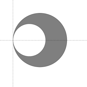
Figure 1.1: The eigenvalue spectrum of GW Dirac operators in the complex plane. In the case $R\propto 1$ the spectrum lies exactly on a circle (left), whereas in the general case the spectrum is bounded by two circles and lies in the shaded area (right).

The Dirac operator $\operatorname{\textfrak{D}}$ can always be rescaled as follows

$$(2R)^{1/2}\operatorname{\textfrak{D}}(2R)^{1/2}=\operatorname{{\cal D}}\,,$$ (1.22)

which is often very convenient to derive relations in a simpler way and therefore we will use $\operatorname{{\cal D}}$ in our following discussion; even though all the results – with the obvious modifications – are also valid for $\operatorname{\textfrak{D}}$. The rescaled FP solution is denoted by $\operatorname{{\cal D}_{\rm FP}}$.

In order to see that the GW relation is indeed equivalent to chiral symmetry with a non-zero lattice spacing, we perform an infinitesimal change of variables $\psi\to\psi+i\epsilon\delta\psi$ and $\overline{\psi}\to\overline{\psi}+i\epsilon\delta\overline{\psi}$ with a global flavor singlet transformation [21]

$$\delta\psi = \gamma_{5}\left(1-\frac{1}{2}\operatorname{{\cal D}}\right)\psi$$ (1.23)

$$\delta\overline{\psi} = \overline{\psi}\left(1-\frac{1}{2}\operatorname{{\cal D}}\right)\gamma_{5}\,.$$

From the GW relation eq. (1.20) it follows that the action ${\cal A}_{f}=\overline{\psi}\operatorname{{\cal D}}\psi$ is invariant under this transformation, i.e.

$$\delta(\overline{\psi}\operatorname{{\cal D}}\psi)=0\,.$$ (1.24)

The corresponding flavor non-singlet transformation is given by

$$\delta_{a}\psi = T_{a}\gamma_{5}\left(1-\frac{1}{2}\operatorname{{\cal D}}\right)\psi\,,$$ (1.25)

$$\delta_{a}\overline{\psi} = \overline{\psi}\left(1-\frac{1}{2}\operatorname{{\cal D}}\right)\gamma_{5}T_{a}\,.$$

Analogous to Fujikawa’s observation discussed in Section 1.1 the fermionic integration measure is not invariant under the singlet transformation in eq. (1.23)

$$\delta[d\overline{\psi}d\psi] = {\rm Tr}(\gamma_{5}\operatorname{{\cal D}})[d\overline{\psi}d\psi]$$

$$= 2N_{\rm f}(n_{\rm L}-n_{\rm R})[d\overline{\psi}d\psi]\,,$$

where the trace Tr denotes the trace over all indices, i.e. color, flavor, Dirac and spatial indices. To derive eq. (1.2.2) we make use of the lattice version of the Atiyah-Singer index theorem [42]. Hence, the measure breaks the flavor singlet chiral symmetry in a topologically non-trivial gauge field where the ${\rm index}(\operatorname{{\cal D}})=n_{\rm L}-n_{\rm R}\neq 0$. Before we discuss the index theorem in more detail, let us mention that the non-singlet symmetry is not anomalous, since eq. (1.2.2) for this case contains ${\rm Tr}(\gamma_{5}\operatorname{{\cal D}}T)\propto{\rm tr}(T)=0$.

Having a Dirac operator satisfying the GW relation one can easily show that the following identity, the lattice index theorem, holds

$${\rm index}(\operatorname{{\cal D}})=\frac{1}{2}{\rm Tr}(\gamma_{5}\operatorname{{\cal D}})\,.$$ (1.27)

Furthermore, one can derive

$$\frac{1}{2}{\rm tr}(\gamma_{5}\operatorname{{\cal D}})\,\to\frac{1}{32\pi^{2}}F^{a}_{\mu\nu}\tilde{F}^{a}_{\mu\nu}$$ (1.28)

in the continuum limit [47, 49]. This shows that the index of the lattice Dirac operator is indeed connected to the topological charge or winding number of the gauge fields (see also eqs. (1.9) and (1.10)). Moreover, the index theorem provides a new definition for the topological charge density on the lattice, namely

$$q(x)=\frac{1}{2}{\rm tr}(\gamma_{5}\operatorname{{\cal D}}(x,x))\,,$$ (1.29)

where the trace is over Dirac and color indices.

It has been shown that GW Dirac operators can not be ultra-local [81, 82, 83, 84], i.e. their couplings $\rho(x-y)$ can not vanish for all $|x-y|>r$ for any finite $r$. This fact is more a technical than a fundamental problem in simulations, because the couplings of the Dirac operator – at least for any acceptable solution of the GW relation, such as the FP Dirac operator – fall off exponentially. Such Dirac operators are still local in a physical sense, as the localization range of the couplings measured in physical units shrinks to 0 in the continuum limit. However, the fact that no ultra-local solutions exist already gives a hint that it is not easy to find an approximation to a GW fermion that can be used in numerical simulations. But let us discuss now one of the solutions of the GW relation, the FP Dirac operator and the FP approach to QCD, more in detail.

1.3 The Renormalization Group and Fixed Point Actions

Field Theories are defined over a large range of scales. However, not all the scales are equally important for the underlying physics. Whereas the low energy excitations carry the information on the long range properties of the theory, the degrees of freedom associated with very high (and unphysical) scales do influence the physical predictions only indirectly through a complex cascade process. This makes the connection between the local form of the interaction described by the Lagrangian and the final physical predictions obscure and, moreover, introduces technical difficulties in treating the large number of degrees of freedom. That is the reason why one attempts to separate the low energy scales from the scales associated with very high energies by integrating them out in the path integral. The method accomplishing this, taking into account the effect on the remaining variables exactly, is called the Renormalization Group transformation (RGT) [18, 85, 86, 87, 88, 89, 90, 91].

The repeated use of the RGT on an initial theory gives a sequence of theories. These theories can be described by a flow trajectory in the space of couplings. Fixed points (FP) of this transformation are theories that reproduce itself under the RGT. Since the correlation length $\xi$ of the theory scales by the scaling factor of the RGT, its value has to be 0 or $\infty$ at the fixed point. Yang-Mills theory has a non-trivial fixed point (the Gaussian FP) with correlation length $\xi=\infty$ whose exact location in coupling space $c_{1}$, $c_{2},\ldots$ depends on the RGT used. There is one so-called relevant coupling whose strength increases as one is starting near this FP and performing RGTs. In QCD the quark masses are additional relevant couplings of the RGT. The flow along these relevant scaling fields whose end-point is the FP is called the renormalized trajectory (RT). Simulations performed using an action which is on the exact RT would reproduce continuum physics without any discretization errors. Let us finally mention that a detailed review on FP actions can be found in [92].

1.3.1 Fixed Point Action of QCD

We consider the QCD Lagrangian which consists of a SU(3) non-abelian gauge theory and a fermionic part describing the quarks in interaction with the gauge fields in four dimensional Euclidean space defined on a periodic lattice. The partition function is defined through

$${\cal Z}(\beta)=\int DUD\bar{\psi}D\psi\exp[-\beta{\cal A}_{g}(U)-{\cal A}_{f}(U,\bar{\psi},\psi)],$$ (1.30)

where $DU$ is the invariant group measure, $D\bar{\psi}D\psi$ the (anti)fermion integration measure and $\beta$ the gauge coupling. The lattice actions ${\cal A}_{g}(U)$ and ${\cal A}_{f}(U,\bar{\psi},\psi)$ are some lattice regularizations of the corresponding continuum gauge and fermion action, respectively. We can perform a real space renormalization group transformation (RGT),

$$\exp[-(\beta^{\prime}{\cal A}_{g}^{\prime}(V)+{\cal A}_{f}^{\prime}(V,\bar{\chi},\chi))]=\\ \int DUD\bar{\psi}D\psi\exp[-\{\beta({\cal A}_{g}(U)+T_{g}(U,V))+({\cal A}_{f}(U,\bar{\psi},\psi)+T_{f}(U,\bar{\chi},\chi,\bar{\psi},\psi))\}],$$ (1.31)

where $V$ is the blocked link variable, $\chi$ and $\bar{\chi}$ the blocked fermion fields. Finally, $T_{g}(U,V)$ and $T_{f}(U,\bar{\chi},\chi,\bar{\psi},\psi)$ are the blocking kernels defining the RGT,

$$T_{g}(U,V)=-\frac{\kappa_{g}}{N}\sum_{n_{B},\mu}\left(\text{Re}\,\text{tr}(V_{\mu}(n_{B})Q^{\dagger}_{\mu}(n_{B}))-{\cal N}_{\mu}^{\beta}\right)$$ (1.32)

and

$$T_{f}(U,\bar{\chi},\chi,\bar{\psi},\psi)=\kappa_{f}\sum_{n_{B}}\big{(}\bar{\chi}_{n_{B}}-\sum_{n}\bar{\psi}_{n}\Omega^{\dagger}(U)_{n,n_{B}}\big{)}\\ \times\big{(}\chi_{n_{B}}-\sum_{n}\Omega(U)_{n_{B},n}\psi_{n}\big{)}.$$ (1.33)

In eq. (1.32) $Q_{\mu}(n_{B})$ is a $3\times 3$ matrix representing some mean of products of link variables $U_{\mu}(n)$, connecting the sites $2n_{B}$ and $2(n_{B}+\hat{\mu})$ on the fine lattice and ${\cal N}_{\mu}^{\beta}$ is a normalization constant ensuring the invariance of the partition function. By optimizing the averaging function in $Q_{\mu}$ and the parameter $\kappa_{g}$, it is possible to obtain an action on the coarse lattice, which has a short interaction range. Such an optimization has been done and we refer to [93] for the explicit form of the RGT block transformation.

The fermionic blocking kernel in eq. (1.33) is defined by the averaging function $\Omega(U)_{n_{B},n}$, which connects the fermion fields on the fine lattice $\psi$ to the fermion fields on the coarse lattice $\chi$. It is a generic gauge invariant function with hypercubic symmetry that on trivial gauge configurations satisfies the normalization condition $\sum_{n}\Omega(2n_{B}-n)=2^{\frac{d-1}{2}}$ for $d$ space-time dimensions.

On the critical surface at $\beta\rightarrow\infty$ eq. (1.31) is dominated by the gauge part and it becomes a saddle point problem representing an implicit equation for the FP action, ${\cal A}_{g}^{\text{FP}}$,

$${\cal A}_{g}^{\text{FP}}(V)=\min_{\{U\}}\left\{{\cal A}_{g}^{\text{FP}}(U)+T(U,V)\right\}.$$ (1.34)

The normalization constant in the blocking kernel, ${\cal N}_{\mu}^{\beta}$, becomes in the limit $\beta\rightarrow\infty$

$${\cal N}_{\mu}^{\infty}=\max_{W\epsilon\text{SU}(3)}\left\{\text{Re}\,\text{tr}(WQ\mu^{\dagger})\right\}.$$ (1.35)

Note that the FP eq. (1.34) defines the FP gauge action as well as the field on the fine configuration $U[V]$ implicitly through a minimization condition.

As the gauge part completely dominates the path integral for large values of the gauge coupling $\beta$, the fermionic part does not have any influence on the solution of the FP gauge action. This is, however, completely different for the fermionic FP action as the gauge fields on the fine as well on the coarse lattice show up in the fermionic FP equation [94]

$$\textfrak{D}_{\rm FP}^{-1}(V)=\frac{1}{\kappa_{f}}+\Omega(U[V])\textfrak{D}_{\rm FP}^{-1}(U[V])\Omega^{\dagger}(U[V])$$ (1.36)

or equivalently

$$\operatorname{\textfrak{D}_{\rm FP}}(V)=\kappa_{f}-\kappa_{f}^{2}\Omega(U[V])[\operatorname{\textfrak{D}_{\rm FP}}(U[V])+\kappa_{f}\Omega^{\dagger}(U[V])\Omega(U[V])]^{-1}\Omega^{\dagger}(U[V])\,.$$ (1.37)

Combining eq. (1.36) with the GW relation from eq. (1.2), we obtain the following FP equation for the operator $R$ appearing in the GW relation

$$R_{\rm FP}(V)=\frac{1}{\kappa_{f}}+\Omega(U[V])R_{\rm FP}(U[V])\Omega^{\dagger}(U[V])\,.$$ (1.38)

The FP eqs. (1.34), (1.36), (1.37) and (1.38), respectively, can be studied analytically up to quadratic order in the vector potentials [93, 94]. However, for solving the FP equations on coarse configurations with large fluctuations – as they are needed for numerical simulations in QCD – one has to resort to numerical methods, and a sufficiently rich parametrization for the description of the solution is required. The numerical solution of the eq. (1.34) defining the FP gauge action is described in [95, 96], whereas a substantial part of this work is devoted to the numerical solution of the fermionic FP eqs. (1.36) and (1.37). But before we give an account of the parametrization problem, we first discuss the properties of a general Dirac operator, because we need a Dirac operator with a rich structure to be able to capture some of the very important properties of the FP Dirac operator.

Chapter 2 General Lattice Dirac Operator

In this chapter we discuss the steps to construct Dirac operators which have arbitrary fermion offsets, gauge paths, a general structure in Dirac space and satisfy the basic symmetries on the lattice, which are gauge symmetry, hermiticity condition, charge conjugation, hypercubic rotations and reflections. We give an extensive set of examples and provide an efficient factorization of the operators occurring in the construction of a Dirac operator. Although the discussion about the lattice Dirac operators is kept very general, all the examples are specific to the construction of the parametrized FP Dirac operator $\operatorname{\textfrak{D}_{\rm par}}$, which we discuss in Chapter 3.

2.1 Introduction

The construction of a general lattice Dirac operator that satisfies all the basic symmetries (gauge symmetry, $\gamma_{5}$ hermiticity, charge conjugation, hypercubic rotations and reflections) is a fundamental kinematic problem. We discuss this problem in $d=4$ in a very general way. Notice that a similar discussion with different notation can be found in [22, 24]. For any fermion offset and for any of the 16 elements of the Clifford algebra we describe the steps to find combinations of gauge paths which satisfy all the basic symmetries. We construct explicitly paths for all the elements of the Clifford algebra in the offsets of the hypercube. We show also how to factorize the sum of paths, i.e. writing it as a product of sums, in such a way that the computational problem is manageable even if the number of paths is large.

Most of the contents of this chapter are published in [67] as well as in hep-lat/0003013, where an easy-to-use Maple code dirac.maple is provided. This code can be used, if one wants to add additional terms to a parametrization of a Dirac operator.

Let us add a few remarks at this point:

1. There are many ways to fix the parameters of the chosen Ansatz for the Dirac operator. As opposed to production runs this problem should be treated only once. It is useful to invest effort here, since the choice will influence strongly the quality of the results in simulations.

2. There are compelling reasons to use the elements of the Clifford algebra beyond $1$ and $\gamma^{\mu}$ in the Dirac operator. For an operator $\operatorname{\textfrak{D}}$ satisfying the GW relation in eq. (1.1), $\,\hbox{tr}\,(\gamma_{5}R\operatorname{\textfrak{D}})$ is the topological charge density [42, 21], i.e. the $\gamma_{5}$ part of $\operatorname{\textfrak{D}}$ is obviously important. Similarly, a $\sigma^{\mu\nu}$ term is already required by the leading Symanzik condition.

3. If the parametrization is close to $\operatorname{\textfrak{D}_{\rm FP}}$, the GW relation is approximately satisfied, which means the operator $A^{\dagger}A$ under the square root in Neuberger’s overlap construction is close to $1$. An expansion converges very fast in this case, as we will show in Chapter 5. In the present situation it is, however, unclear whether this speed-up of the convergence compensates for additional expenses of the improved operator [33, 97, 98]. But, there are many reasons to use improved Dirac operators and performance issues in the overlap construction are most likely not more important than good scaling properties of the resulting operator.

4. The basic numerical operation in production runs is $\operatorname{\textfrak{D}_{\rm par}}\eta$, where $\operatorname{\textfrak{D}_{\rm par}}$ is the parameterized Dirac matrix and $\eta$ is a vector. The matrix elements of $\operatorname{\textfrak{D}_{\rm par}}$ should be precalculated before the iteration starts. Using all the Clifford algebra elements and arbitrary gauge paths, the computational cost per offset of the operation $\operatorname{\textfrak{D}_{\rm par}}\eta$ is a factor of $\sim 4$ higher than that of the Wilson action. Using all the points of the hypercube (81 offsets), the cost per iteration is increased by a factor of $4\times 81/8\sim 40$ relative to the Wilson Dirac operator. Note however, that this number may vary quite a bit depending on the underlying computer architecture, as one of the main issues in present lattice simulations is rather fast memory access and fast communication than fast floating point units [99].

2.2 Symmetries of the Dirac Operator

We define the basis of the Clifford algebra as $\Gamma=1,\,\gamma_{\mu},\,i\sigma_{\mu\nu},\,\gamma_{5},\,\gamma_{\mu}\gamma_{5}$. We use the notation S,V,T,P and A for the scalar, vector, tensor, pseudoscalar and axial-vector elements of the Clifford algebra, respectively. Notice that the tensor (T) and axial-vector (A) basis elements of the Clifford algebra are anti-hermitian as one can see from the explicit representation given in Appendix A. It will later be useful to list the basis elements of the Clifford algebra by a single index, as $\Gamma_{i}$, $i=1,\ldots,16$. We choose the ordering

$$\Gamma_{i}=1,\gamma_{1},\gamma_{2},\gamma_{3},\gamma_{4},i\sigma_{12},i\sigma_{13},i\sigma_{14},i\sigma_{23},i\sigma_{24},i\sigma_{34},\gamma_{5},\gamma_{1}\gamma_{5},\gamma_{2}\gamma_{5},\gamma_{3}\gamma_{5},\gamma_{4}\gamma_{5}.$$ (2.1)

Under charge conjugation, the Dirac matrices $\gamma_{\mu}$ transform as

$${\cal C}\gamma_{\mu}^{T}{\cal C}^{-1}=-\gamma_{\mu}\,.$$ (2.2)

Having chosen the T and A basis elements of the Clifford algebra to be anti-hermitian, all the basis elements have the property that

$${\cal C}\gamma_{5}\Gamma^{*}\gamma_{5}{\cal C}^{-1}=\Gamma\,.$$ (2.3)

We define a sign $\epsilon_{\Gamma}$ by the relation

$$\gamma_{5}\Gamma^{\dagger}\gamma_{5}=\epsilon_{\Gamma}\Gamma,$$ (2.4)

which gives $\epsilon_{\rm S}=\epsilon_{\rm P}=\epsilon_{\rm A}=1$ and $\epsilon_{\rm V}=\epsilon_{\rm T}=-1$.

Under reflection of the coordinate axis $\eta$, the basis elements of the Clifford algebra are transformed as $\Gamma^{\prime}={\cal P}_{\eta}\Gamma{\cal P}_{\eta}^{-1}$, where ${\cal P}_{\eta}=\gamma_{\eta}\gamma_{5}$. (When $\Gamma$ is written in terms of Dirac matrices $\gamma_{\mu}$ this amounts simply to reversing the sign of $\gamma_{\eta}$.) The group of reflections has $2^{4}=16$ elements. Under a permutation $(1,2,3,4)\to(p_{1},p_{2},p_{3},p_{4})$ of the coordinate axes the basis elements of the Clifford algebra transform by replacing $\mu\to p_{\mu}$ and accordingly $\gamma_{5}\to\epsilon_{p_{1}p_{2}p_{3}p_{4}}\gamma_{5}$.

The matrix elements of the Dirac operator $D$ we denote as

$$D(n,n^{\prime};U)_{\alpha\alpha^{\prime}}^{aa^{\prime}}$$ (2.5)

where $n$, $a$ and $\alpha$ refer to the coordinate, color and Dirac indices, respectively. From now on, we suppress the color and Dirac indices. The gauge configuration $U$ appearing in $D$ is not necessarily the original one entering the gauge action – it could be a smeared configuration $V$. Using the Dirac operator $D(V)$ should be interpreted as defining a new Dirac operator $D^{\prime}$ on the thermally generated configuration $U$: $D^{\prime}(U)=D(V)$, where $D^{\prime}$ has a large number of additional paths relative to $D$. Provided the smearing has appropriate symmetry properties all the following constructions in this chapter remain valid, without any extra modifications.

The Dirac operator should satisfy the following symmetry requirements:

Gauge symmetry

Under the gauge transformation $U_{\mu}(n)\rightarrow U_{\mu}(n)^{g}=g(n)\,U_{\mu}(n)\,g(n+\hat{\mu})^{\dagger}$, where $g(n)\in{\rm SU}(N)$ we have

$$D(n,n^{\prime};U)\rightarrow\,D(n,n^{\prime};U^{g})=g(n)\,D(n,n^{\prime};U)\,g(n^{\prime})^{\dagger}.$$ (2.6)

Translation invariance

Translation symmetry requires that $D(n,n+r)$ depends on $n$ only through the $n$-dependence of the gauge fields. There is no explicit $n$-dependence beyond that. In particular, the coefficients in front of the different paths which enter $D$ do not depend on $n$.

Hermiticity

$$D(n,n^{\prime};U)=\gamma_{5}\,D(n^{\prime},n,U)^{\dagger}\,\gamma_{5},$$ (2.7)

where $\dagger$ is hermitian conjugation in color and Dirac space.

Charge conjugation

$$D(n,n^{\prime};U)={\cal C}\,D(n^{\prime},n;U^{*})^{T}\,{\cal C}^{-1}\,,$$ (2.8)

where $T$ is the transpose operation in color and Dirac space.

It will be useful to combine eqs. (2.7) and (2.8) to obtain

$$D(n,n^{\prime};U)={\cal C}\gamma_{5}\,D(n,n^{\prime};U^{*})^{*}\,\gamma_{5}{\cal C}^{-1}\,.$$ (2.9)

Reflection of the coordinate axis $\eta$

$$D(n,n^{\prime};U)={\cal P}^{-1}_{\eta}\,D(\tilde{n},\tilde{n}^{\prime};U^{{\cal P}_{\eta}})\,{\cal P}_{\eta}\,,$$ (2.10)

where ${\cal P}_{\eta}=\gamma_{\eta}\gamma_{5}$ and $\tilde{n}_{\nu}=n_{\nu}$ if $\nu\neq\eta$, while $\tilde{n}_{\eta}=-n_{\eta}$. The reflected gauge field $U^{{\cal P}_{\eta}}$ is defined as

$$U^{{\cal P}_{\eta}}_{\eta}(m) = U_{\eta}(\tilde{m}-\hat{\eta})^{\dagger}\,,$$ (2.11)

$$U^{{\cal P}_{\eta}}_{\nu}(m) = U_{\nu}(\tilde{m})\,,\qquad\nu\neq\eta.$$

Permutation of the coordinate axes

These are defined in a straightforward way, by permuting the Lorentz indices appearing in $D$. Note that rotations by $90^{\circ}$ on a hypercubic lattice can be replaced by reflections and permutations of the coordinate axes.

2.3 Constructing a Matrix $D$ which satisfies the Symmetries

To describe a general Dirac operator in compact notations, it is convenient to introduce the operator $\hat{U}_{\mu}$ of the parallel transport for direction $\mu$

$$\left(\hat{U}_{\mu}\right)_{nn^{\prime}}=U_{\mu}(n)\delta_{n+\hat{\mu},n^{\prime}}\,,$$ (2.12)

and analogously for the opposite direction

$$\left(\hat{U}_{-\mu}\right)_{nn^{\prime}}=U_{\mu}(n-\hat{\mu})^{\dagger}\delta_{n-\hat{\mu},n^{\prime}}\,.$$ (2.13)

Obviously $\left(\hat{U}_{\mu}\right)^{\dagger}=\hat{U}_{-\mu}$. The Wilson Dirac operator at bare mass equal to zero reads:

$$D_{\rm W}=\frac{1}{2}\sum_{\mu}\gamma_{\mu}\left(\hat{U}_{\mu}-\hat{U}_{\mu}^{\dagger}\right)+\frac{1}{2}r\sum_{\mu}\left(2-\hat{U}_{\mu}-\hat{U}_{\mu}^{\dagger}\right)\,.$$ (2.14)

It is also useful to introduce the operator $\hat{U}(l)$ of the parallel transport along some path $l=[l_{1},l_{2},\ldots,l_{k}]$ where $l_{i}=\pm 1,\ldots,\pm 4$, by

$$\hat{U}(l)=\hat{U}_{l_{1}}\hat{U}_{l_{2}}\ldots\hat{U}_{l_{k}}\,.$$ (2.15)

In terms of gauge links this is

$$\left(\hat{U}(l)\right)_{nn^{\prime}}=\left(U_{l_{1}}(n)U_{l_{2}}(n+\hat{l}_{1})\ldots\right)\delta_{n+r_{l},n^{\prime}}\,,$$ (2.16)

where $r_{l}=\hat{l}_{1}+\ldots+\hat{l}_{k}$ is the offset corresponding to the path $l$. Note that $\hat{U}(l)^{\dagger}=\hat{U}(\bar{l})$ where $\bar{l}=[-l_{k},\ldots,-l_{1}]$ is the inverse path. In particular, one has

$$\left(\hat{U}([2,1,-2])\right)_{nn^{\prime}}=U_{2}(n)U_{1}(n+\hat{2})U_{2}(n+\hat{1})^{\dagger}\delta_{n+\hat{1},n^{\prime}}$$ (2.17)

for the corresponding staple.

As another example, the Sheikholeslami-Wohlert (or clover) term [14] introduced to cancel the ${\cal O}(a)$ artifacts is given up to a constant prefactor by

$$i\sigma_{\mu\nu}\left(\hat{U}([\mu,\nu,-\mu,-\nu])+\hat{U}([\nu,-\mu,-\nu,\mu])+\right.\\ \left.\hat{U}([-\mu,-\nu,\mu,\nu])+\hat{U}([-\nu,\mu,\nu,-\mu])-{\rm h.c.}\right)\,.$$ (2.18)

We consider a general form of the Dirac operator

$$D=\sum_{i}\Gamma_{i}\sum_{l}c^{(i)}_{l}\hat{U}(l)\,.$$ (2.19)

The Dirac indices are carried by $\Gamma_{i}=1,\gamma_{\mu},\ldots$, the coordinate and color indices by the operators $\hat{U}(l)$. The Dirac operator is determined by the set of paths $l$ the sum runs over, and the coefficients $c^{(i)}_{l}$.

In the case of $D_{\rm W}$ (see eq. (2.14)), for $\Gamma=1$ one has $l=[1],[-1],\ldots,[-4]$ and $l=[]$ (the empty path $l=[]$ corresponds to $\hat{U}([])=1$), while for $\Gamma=\gamma_{\mu}$: $l=[\mu]$ and $[-\mu]$. In the clover term, eq. (2.18) for $\Gamma=i\sigma_{\mu\nu}$: $l=[\mu,\nu,-\mu,-\nu],\ldots$ (altogether $6\times 4=24$ plaquette products). As these well known examples indicate, the coefficients $c_{l}^{(i)}$ for related paths differ only in relative signs, which are fixed by symmetry requirements.

Our aim is to give for all $\Gamma$’s and offsets $r$ on the hypercube a set of paths and to determine the relative sign for paths related to each other by symmetry transformations. We give the general rules for arbitrary offsets and paths as well.

Eqs. (2.3,2.9) imply that the coefficients $c_{l}^{(i)}$ in eq. (2.19) are real. Further, from hermiticity in this language it follows that the path $l$ and the opposite path $\bar{l}$ (or equivalently, $\hat{U}(l)$ and $\hat{U}(l)^{\dagger}$) should enter in the combination

$$\Gamma\left(\hat{U}(l)+\epsilon_{\Gamma}\hat{U}(l)^{\dagger}\right)\,,$$ (2.20)

where the sign $\epsilon_{\Gamma}$ is defined by $\gamma_{5}\Gamma^{\dagger}\gamma_{5}=\epsilon_{\Gamma}\Gamma$, eq. (2.4).

The symmetry transformations formulated in terms of matrix elements in the previous section can be translated to the formalism used here. The reflections and permutations act on operators $\hat{U}(l)$ in a straightforward way. Under a reflection of the axis $\eta$ one has $\hat{U}(l)\to\hat{U}(l^{\prime})$ where $l^{\prime}_{i}=-l_{i}$ if $|l_{i}|=\eta$ and unchanged otherwise. Under a permutation $(p_{1},p_{2},p_{3},p_{4})$ a component with $l_{i}=\pm\mu$ is replaced by $l_{i}=\pm p_{\mu}$, as expected. The number of combined symmetry transformations is $16\times 24=384$. We denote the action of a transformation $\alpha=1,\ldots,384$ by $\Gamma\to\Gamma^{(\alpha)}$, $\hat{U}(l)\to\hat{U}(l^{(\alpha)})$. Acting on the expression in eq. (2.20) by all 384 elements of the symmetry group and adding the resulting operators together, the sum will satisfy the required symmetry conditions for a Dirac operator.

Let us introduce the notation

$$\hat{d}(\Gamma,l)=\frac{1}{\cal N}\sum_{\alpha}\Gamma^{(\alpha)}\left(\hat{U}(l^{(\alpha)})+\epsilon_{\Gamma}\hat{U}(l^{(\alpha)})^{\dagger}\right)\,.$$ (2.21)

A general Dirac operator will be a linear combination of such terms, unless one chooses the coefficients to be gauge invariant functions of the gauge fields, which can take different values for different offsets generated by the reference path. We will be more specific about this possibility to extend the construction of a general Dirac operator using color singlet factors. The normalization factor ${\cal N}$ will be defined below. The total number of terms in eq. (2.21) is $2\times 384=768$. Typically, however, the number of different terms which survive after the summation is much smaller. It can happen that for a choice of starting $\Gamma$ and $l$ the sum in eq. (2.21) is zero. In this case the given path does not contribute to the Dirac structure $\Gamma$.

To fix the convention for the overall sign we single out a definite term in the sum of eq. (2.21) and take its sign to be $+1$. Denote by $\Gamma_{0}$, $l_{0}$ the corresponding quantities of this reference term, and by $r_{0}=r(l_{0})$ the offset of $l_{0}$. This term is specified by narrowing down the set $\{\Gamma^{(\alpha)},l^{(\alpha)}\}$ to a single member as follows:

• Given an offset $r=r(l)=(r_{1},r_{2},r_{3},r_{4})$ the reflections and permutations create all offsets $(\pm r_{p_{1}},\ \pm r_{p_{2}},\ \pm r_{p_{3}},\ \pm r_{p_{4}})$ where $(p_{1},p_{2},p_{3},p_{4})$ is an arbitrary permutation. We choose for the reference offset $r_{0}$ the one from the set $\{r(l^{(\alpha)})\}$ which satisfies the relations $r_{01}\geq r_{02}\geq r_{03}\geq r_{04}\geq 0$.

• If several $\Gamma$ matrices are generated to this offset then choose as $\Gamma_{0}$ the one which comes first in the natural order, eq. (2.1).

• Consider all the paths $\{l^{(\alpha)}\}$ having offset $r_{0}$ and associated with $\Gamma_{0}$, i.e. $r(l^{(\alpha)})=r_{0}$ and $\Gamma^{(\alpha)}=\Gamma_{0}$. To single out one path $l_{0}$ from this set, we associate to a path $l=[l_{1},l_{2},\ldots,l_{k}]$ a decimal code $d_{1}d_{2}\ldots d_{k}$ with digits $d_{i}=l_{i}$ if $l_{i}>0$ and $d_{i}=9+l_{i}$ for $l_{i}<0$. The path with the smallest code will be the reference path $l_{0}$. (In other words we take the first in lexical order defined by the ordering $1,2,3,4,-4,-3,-2,-1$.)

Of course, one can take $\Gamma_{0}$, $l_{0}$ as the starting $\Gamma$ and $l$, and we shall refer to the expression in eq. (2.21) as $\hat{d}(\Gamma_{0},l_{0})$ to indicate that it is associated to a class rather than to a specific $(\Gamma,l)$.

We turn now to the normalization of $\hat{d}(\Gamma_{0},l_{0})$. In general, there will be $K$ different paths in the set $\{l^{(\alpha)}\,|\,\Gamma^{(\alpha)}=\Gamma_{0},r(l^{(\alpha)})=r_{0}\}$, i.e. corresponding to the same offset $r_{0}$ and Dirac structure $\Gamma_{0}$. The normalization is fixed by requiring that the coefficient of the reference term $\Gamma_{0}\hat{U}(l_{0})$ is $+1/K$.

Consider a simple example explicitly. Let $r_{0}=(1,0,0,0)$, $\Gamma_{0}=i\sigma_{12}$ and $l_{0}=[2,1,-2]$. The starting term, in eq. (2.20) is $i\sigma_{12}(\hat{U}([2,1,-2])-\hat{U}([2,-1,-2]))$. Applying all the 16 different reflections gives

$$8i\sigma_{12}\left(\hat{U}([2,1,-2])-\hat{U}([2,-1,-2])-\hat{U}([-2,1,2])+\hat{U}([-2,-1,2])\right)\,.$$ (2.22)

Applying all the permutations on this expression results in:

$$\hat{d}(\Gamma_{0},l_{0})=\frac{1}{{\cal N}}\left\{16i\sigma_{12}\left(\hat{U}([2,1,-2])-\hat{U}([-2,1,2])\right)+\right.\\ 16i\sigma_{13}\left(\hat{U}([3,1,-3])-\hat{U}([-3,1,3])\right)+\\ \left.16i\sigma_{14}\left(\hat{U}([4,1,-4])-\hat{U}([-4,1,4])\right)+\ldots\right\}\,,$$ (2.23)

where only the terms with the offset $r=r_{0}$ are written out explicitly. Their total number is 96. The whole generated set has 8 different offsets giving altogether 768 terms. Notice the form of the contribution in eq. (2.23). There is a common factor (16 in this case) multiplying all the different operators. Only the tensor elements of the Clifford algebra enter, since we started with a tensor element. Beyond the common factor the path products have a coefficient $\pm 1$. These features are general. The number of different paths with $\Gamma_{0}=i\sigma_{12}$ and $r_{0}=(1,0,0,0)$ is K=2: the paths $[2,1,-2]$ and $[-2,1,2]$). The normalization factor in this case is ${\cal N}=16\times 2=32$, so that one has $\hat{d}(\Gamma_{0},l_{0})=\frac{1}{2}i\sigma_{12}\left(\hat{U}([2,1,-2])-\hat{U}([-2,1,2])\right)+\ldots$.

A general Dirac operator is constructed as

$$D=\sum_{i=\Gamma_{0},l_{0}}\frac{1}{{\cal N}_{i}}\sum_{\alpha}f_{i}(l^{(\alpha)})\Gamma_{i}^{(\alpha)}\left(\hat{U}(l_{i}^{(\alpha)})+\epsilon_{\Gamma}\hat{U}(l_{i}^{(\alpha)})^{\dagger}\right)\,.$$ (2.24)

The coefficients $f_{i}(l^{(\alpha)})$ which are the free, adjustable parameters of the Dirac operator are real constants or more generally gauge invariant, real functions of the gauge fields, respecting locality, and invariance under the symmetry transformations. The requirement that such a function is gauge invariant and real, restricts the choice to the real part of traces of closed loops of link products. The invariance under symmetry transformations can be assured by constructing these functions along the same lines as a scalar operator which satisfies the symmetry requirements. The following example should make clear what is meant by such a color singlet function. We consider again the coupling generated by the staples and the tensor Clifford algebra elements i.e. $r_{0}=(1,0,0,0)$, $\Gamma_{0}=\rm i\sigma_{12}$ and $l_{0}=[2,1,-2]$. A simple choice for such a function which satisfies all the requirements would e.g. be a polynomial of the trace of all the plaquettes generated by the operator $r_{0}=(0,0,0,0)$, $\Gamma_{0}=1$ and $l_{0}=[1,2,-1,-2]$. But there are other possible choices, such as

$$f(l^{(i)})=f(x(l^{(i)}))$$

with

$$x(l^{(i)})=1-\frac{1}{N_{c}}\,\hbox{tr}\,[X(l^{(i)})X(l^{(i)})^{\dagger}]\,,$$ (2.25)

where $X$ is the gauge operator generated by $r_{0}=(1,0,0,0)$, $\Gamma_{0}=1$ and $l_{0}=[2,1,-2]$, $N_{c}$ the number of colors and $l^{(i)}$, $i=1,\ldots,n_{\rm offsets}$ denotes the different offsets generated by $l_{0}$. This choice gives the possibility that different offsets generated from the same $\Gamma_{0}$ and $l_{0}$ can have different couplings in the sense that the value of the function $f(l^{(i)})$ is not necessarily the same for every offset. In the parametrization of $\operatorname{\textfrak{D}_{\rm FP}}$ and $R$ we always use a linear function

$$f(x(l^{(i)}))=c_{0}+c_{1}x(l^{(i)})$$ (2.26)

for the couplings.

2.4 Tables for Offsets on the Hypercube

Choosing offsets and paths to be included in the Dirac operator is a matter of intuition. It is also influenced by considerations on CPU time and memory requirements. In Tables 2.1-2.5 we give the reference paths $l_{0}$ for offsets on the hypercube and general Dirac structure that are used in the current implementation of the parametrized FP Dirac operator $\operatorname{\textfrak{D}_{\rm par}}$. The first 3 columns give $\Gamma_{0}$, $l_{0}$ and the number of paths $K$ as defined in the previous section. The 4th column gives those Clifford basis elements which are generated in eq. (2.21) to the offset $r_{0}$. In Table 2.6 we give the gauge invariant, real functions of the gauge fields which are used as fluctuation polynomials in the current implementation of $\operatorname{\textfrak{D}_{\rm par}}$.

$\Gamma_{0}$	ref. path $l_{0}$	$K$	$\Gamma$’s generated	$c_{X}$
$1$	$[]$	1	1	$1$, $0$
	$[1,2,-1,-2]$	48		$1$, $0$
$\gamma_{1}$	$[1,2,-1,-2]$	24	$\gamma^{1},\dots,\gamma^{4}$	0
$i\sigma_{12}$	$[1,2,-1,-2]$	8	$i\sigma_{12},\dots,i\sigma_{34}$	$-1$
$\gamma_{5}$	$[1,2,-1,-2,3,4,-3,-4]$	384	$\gamma_{5}$	$-1/6$
	$[1,2,3,4,-1,-2,-3,-4]$	384		$-1/6$
$\gamma_{1}\gamma_{5}$	$[1,2,-1,-2,3,4,-3,-4]$	192	$\gamma_{1}\gamma_{5},\dots,\gamma_{4}\gamma_{5}$	0
	$[2,1,-2,-1,3,4,-3,-4]$	192		0

Table 2.1: Reference paths for different $\Gamma_{0}$’s for offset (0000).

$\Gamma_{0}$	ref. path $l_{0}$	$K$	$\Gamma$’s generated	$c_{X}$
$1$	$[1]$	1	1	$8$, $1$
	$[2,1,-2]$	6		$8$, $1$
	$[2,3,1,-3,-2]$	24		$8$, $1$
$\gamma_{1}$	$[1]$	1	$\gamma_{1}$	$2$
	$[2,1,-2]$	6		$2$
$\gamma_{2}$	$[1,2,3,-2,-3]$	16	$\gamma_{2},\gamma_{3},\gamma_{4}$	$0$
$i\sigma_{12}$	$[2,1,-2]$	2	$i\sigma_{12},i\sigma_{13},i\sigma_{14}$	$4$
$i\sigma_{23}$	$[1,2,3,-2,-3]$	16	$i\sigma_{23},i\sigma_{24},i\sigma_{34}$	$-4$
$\gamma_{5}$	$[2,1,-2,3,4,-3,-4]$	96	$\gamma_{5}$	$4/3$
$\gamma_{1}\gamma_{5}$	$[2,1,-2,3,4,-3,-4]$	96	$\gamma_{1}\gamma_{5}$	$0$
$\gamma_{2}\gamma_{5}$	$[1,3,4,-3,-4]$	16	$\gamma_{2}\gamma_{5},\gamma_{3}\gamma_{5},\gamma_{4}\gamma_{5}$	$-2$

Table 2.2: Reference paths for different $\Gamma_{0}$’s for offset (1000).

$\Gamma_{0}$	ref. path $l_{0}$	$K$	$\Gamma$’s generated	$c_{X}$
$1$	$[1,2]$	2	1	$24$, $6$
$\gamma_{1}$	$[1,2]$	2	$\gamma_{1},\gamma_{2}$	$12$
$\gamma_{3}$	$[1,3,2,-3]$	8	$\gamma_{3},\gamma_{4}$	$0$
$i\sigma_{12}$	$[1,2]$	2	$i\sigma_{12}$	$-2$
$i\sigma_{13}$	$[1,3,2,-3]$	4	$i\sigma_{13},i\sigma_{14},i\sigma_{23},i\sigma_{24}$	$0$
$i\sigma_{34}$	$[1,2,3,4,-3,-4]$	32	$i\sigma_{34}$	$-4$
$\gamma_{5}$	$[1,2,3,4,-3,-4]$	32	$\gamma_{5}$	$-2$
$\gamma_{1}\gamma_{5}$	$[1,2,3,4,-3,-4]$	16	$\gamma_{1}\gamma_{5},\gamma_{2}\gamma_{5}$	$4$
$\gamma_{3}\gamma_{5}$	$[1,4,2,-4]$	8	$\gamma_{3}\gamma_{5},\gamma_{4}\gamma_{5}$	$-4$

Table 2.3: Reference paths for different $\Gamma_{0}$’s for offset (1100).

$\Gamma_{0}$	ref. path $l_{0}$	$K$	$\Gamma$’s generated	$c_{X}$
$1$	$[1,2,3]$	6	1	$32$, $12$
$\gamma_{1}$	$[1,2,3]$	4	$\gamma_{1},\gamma_{2},\gamma_{3}$	$24$
$\gamma_{4}$	$[1,2,4,3,-4]$	24	$\gamma_{4}$	$0$
$i\sigma_{12}$	$[1,2,3]$	4	$i\sigma_{12},i\sigma_{13},i\sigma_{23}$	$-8$
$i\sigma_{14}$	$[1,4,2,-4,3]$	8	$i\sigma_{14},i\sigma_{24},i\sigma_{34}$	$0$
$\gamma_{5}$	$[1,4,2,-4,3]$	12	$\gamma_{5}$	$-8/3$
$\gamma_{1}\gamma_{5}$	$[1,4,2,-4,3]$	8	$\gamma_{1}\gamma_{5},\gamma_{2}\gamma_{5},\gamma_{3}\gamma_{5}$	$8$
$\gamma_{4}\gamma_{5}$	$[1,2,3]$	6	$\gamma_{4}\gamma_{5}$	$-4/3$

Table 2.4: Reference paths for different $\Gamma_{0}$’s for offset (1110).

$\Gamma_{0}$	ref. path $l_{0}$	$K$	$\Gamma$’s generated	$c_{X}$
$1$	$[1,2,3,4]$	24	1	$16$, $8$
$\gamma_{1}$	$[1,2,3,4]$	12	$\gamma^{1},\dots,\gamma^{4}$	$16$
$i\sigma_{12}$	$[1,2,3,4]$	8	$i\sigma_{12},\dots,i\sigma_{34}$	$-8$
$\gamma_{5}$	$[1,2,3,4]$	24	$\gamma_{5}$	$-2/3$
$\gamma_{1}\gamma_{5}$	$[1,2,3,4]$	12	$\gamma_{1}\gamma_{5},\dots,\gamma_{4}\gamma_{5}$	$8/3$

Table 2.5: Reference paths for different $\Gamma_{0}$’s for offset (1111).

offset	ref. path $l_{0}$	K
$(0000)$	$[1,2,-1,-2]$	48
$(1000)$	$[2,1,-2]$	6
$(1100)$	$[1,2]$	2
$(1110)$	$[1,2,3]$	6
$(1111)$	$[1,2,3,4]$	24

Table 2.6: Reference paths for the fluctuation polynomials as defined in eqs. (2.24) and (2.25). Note however, that the fluctuation polynomial for the offset $(1000)$ in the current implementation of the operator $R$ differs from the one given in this table. It is given by the trace of the sum of the plaquettes along a particular link $U(l^{(i)})$ i.e. $x(l^{(i)})=1-1/N_{c}{\rm Re}\,\,\hbox{tr}\,[X(l^{(i)})U(l^{(i)})^{\dagger}]$, where $N_{c}$ is the number of colors and the operator $X$ is given by the operator for the offset $(1000)$ in this table.

It is also of interest how the given Dirac operator behaves for smooth gauge fields, i.e. to obtain the leading terms in the formal continuum limit. The expression in eq. (2.21) generated by given $\Gamma_{0}$ and $l_{0}$ contributes in this limit to one of the expressions (of type S,V,T,P,A) below

$$\left(\bar{c}_{\rm S}+c_{\rm S}\partial^{2}\right)\,;\quad c_{\rm V}\gamma_{\mu}\partial_{\mu}\,;\quad c_{\rm T}\frac{1}{2}\sigma_{\mu\nu}F_{\mu\nu}\,;\\ c_{\rm P}\frac{1}{4}\gamma_{5}\epsilon_{\mu\nu\rho\sigma}F_{\mu\nu}F_{\rho\sigma}\,;\quad c_{\rm A}i\gamma_{\mu}\gamma_{5}\epsilon_{\mu\nu\rho\sigma}\partial_{\nu}F_{\rho\sigma}\,.$$ (2.27)

Here $\partial_{\mu}$ is the covariant derivative in the continuum. The coefficients $c_{X}(\Gamma_{0},l_{0})$, which determine the continuum behavior of the Dirac operator, are presented in the last column of Tables 2.1-2.5. For $\Gamma_{0}=1$ the first and second entries correspond to $\bar{c}_{\rm S}$ and $c_{\rm S}$, respectively. We list their meaning below.

Introduce the notation

$$C_{X}=\sum_{\Gamma_{0},l_{0}}f(\Gamma_{0},l_{0})c_{X}(\Gamma_{0},l_{0})\,,$$ (2.28)

where $f(\Gamma_{0},l_{0})$ is the formal continuum limit of $f_{i}(l^{(\alpha)})$ defined in eq. (2.24). The bare mass $m_{0}$ is given by

$$\bar{C}_{\rm S}=m_{0}\,.$$ (2.29)

The normalization condition on the $D\sim\gamma_{\mu}\partial_{\mu}$ term in $D$ gives

$$C_{\rm V}=1\,.$$ (2.30)

The ${\cal O}(a)$ tree level Symanzik condition reads

$$C_{\rm S}+C_{\rm T}=0\,.$$ (2.31)

The coefficient $C_{\rm P}$ is interesting if the parametrization attempts to describe (approximately) a GW fermion. In this case it is related to the topological charge density $\,\hbox{tr}\,(\gamma_{5}\operatorname{\textfrak{D}}R)$ (see Section 1.2.2),

$$\sum_{\Gamma_{0},l_{0}}f(\Gamma_{0},l_{0})c_{\rm P}(\Gamma_{0},l_{0})R_{\rm free}(r_{0})=\epsilon_{5}\frac{1}{32\pi^{2}}\,.$$ (2.32)

Of course, in the expressions above $\Gamma_{0}$ should be of the corresponding type (S,T,…). The operator $R_{\rm free}(r_{0})$, whose couplings of are specified in Appendix C, is given by $R(n,n+r_{0};U=1)$ of the GW relation eq.(1.1) and $\epsilon_{5}$ is defined through

$$\gamma_{5}=\epsilon_{5}\gamma_{1}\gamma_{2}\gamma_{3}\gamma_{4}\,,$$ (2.33)

which means that $\epsilon_{5}=-1$ for our choice of the Clifford algebra elements (see Appendix A). The relation (2.32) can be derived easily from the work of Fujikawa in [47]. In the parametrization of $\operatorname{\textfrak{D}_{\rm FP}}$ we make use of the relations (2.29)-(2.32) to constrain some of the parameters in the formal continuum limit (see Section 3.2.2).

2.5 Factorizing the Paths

As the Tables 2.1-2.5 show the number of paths, in particularly for the offset $r_{0}=(0,0,0,0)$, is large. It is important to calculate the path products efficiently. An obvious method is to factorize the paths, i.e. to write the sum of a large number of paths as a product of sums over shorter paths. We shall try to factorize in such a way that these shorter paths are mainly plaquette, or staple products.

Because this factorization is a very technical issue, we defer the detailed discussion of the factorization of all the paths involved in the construction of $\operatorname{\textfrak{D}_{\rm par}}$ and $R$ to Appendix B. We however explain the idea on a simple example. Consider the contribution generated by $r_{0}=(0,0,0,0)$, $\Gamma_{0}=\gamma_{5}$ and $l_{0}=[1,2,-1,-2,3,4,-3,-4]$. It contains together with its hermitian conjugate 768 different paths of length 8. The sum over all these terms can, however, be written as

$$\frac{1}{384}\gamma_{5}\left.\sum_{\mu\nu\rho\sigma}\right.^{\prime}\frac{1}{4}\epsilon_{\mu\nu\rho\sigma}P^{\rm(as)}_{\mu\nu}P^{\rm(as)}_{\rho\sigma}\,,$$ (2.34)

with

$$P^{\rm(as)}_{\mu\nu}=P^{(--)}_{\mu,\nu}-{\rm h.c.}$$

$$P^{(--)}_{\mu,\nu}=P_{\mu,\nu}-P_{\mu,-\nu}-P_{-\mu,\nu}+P_{-\mu,-\nu}\,,$$

where $P_{\mu,\nu}$ is the plaquette in the $\mu\nu$-direction, which is a path of length 4. Hence, the whole contribution can be written as the sum of 24 different products of plaquette combinations. The reduction in computational expense in comparison to the calculation of all the 768 length 8 paths is obvious. The observation that the plaquette combinations $P^{\rm(as)}_{\mu\nu}$, as well as other combinations of plaquettes and staples, appear also in other path factorizations makes it favourable to precalculate them on the whole lattice, before one starts to build up the Dirac operator, thereby making the concept of factorizing the paths even more attractive.

Using the factorization of paths the building of the matrix $\operatorname{\textfrak{D}_{\rm par}}$ with all its $41$ different terms and linear fluctuation polynomials in Tables (2.1)-(2.6) is as expensive as ${\cal O}(20)$ matrix vector multiplications with $\operatorname{\textfrak{D}_{\rm par}}$ on PC’s and Alpha workstations. On supercomputers, like the Hitachi SR8000 in Munich, the cost of building the operator is no longer as favourable, since such machines can optimize the matrix vector multiplication much more efficiently and therefore the cost of the building of $\operatorname{\textfrak{D}_{\rm par}}$ is as expensive as ${\cal O}(500)$ matrix vector multiplications. Such a cost becomes a noticeable fraction ($10-20\%$) of the calculation of a full quark propagator. This shows that the factorization of the paths is crucial in order to have a Dirac operator whose build-up time is in a range where it is computationally still reasonable.

Chapter 3 Parametrization of the FP Dirac Operator

The construction of a FP Dirac operator $\operatorname{\textfrak{D}_{\rm FP}}$ is a non-trivial task, since it is defined through a highly non-linear Renormalization Group equation. While the solution can be calculated analytically in the free case [94], this is clearly not possible for the interacting case. Therefore, one has to find a way to approximate the solution as well as possible, always keeping in mind that the resulting Dirac operator shouldn’t be too expensive for practical use. In the following, we describe the details of our construction of an approximation to $\operatorname{\textfrak{D}_{\rm FP}}$. We choose to approximate $\operatorname{\textfrak{D}_{\rm FP}}$ by a general parametrization of a hypercubic Dirac operator as described in Chapter 2. It is clear that such a hypercubic parametrization, which we denote by $\operatorname{\textfrak{D}_{\rm par}}$, is quite a drastic reduction compared to $\operatorname{\textfrak{D}_{\rm FP}}$, which has an infinite number of couplings, like any other Dirac operator satisfying the GW relation [81, 82, 83, 84]. Results from e.g. the O(3) $\sigma$-model, however, support the hope that a compact parametrization which encodes the main features of the full FP operator can be found [100]. The use of a parametrization that contains the full Clifford algebra is a very natural choice for the parametrization of $\operatorname{\textfrak{D}_{\rm FP}}$, since all the Clifford elements are generated through the RGT in eq. (1.37); a fact which was already noticed in [101, 94]. Furthermore, important properties of Dirac operators satisfying the GW relation, like that the topological charge density is given by ${\rm tr}(\gamma_{5}R\operatorname{\textfrak{D}})$, imply that the full Clifford algebra is necessary to achieve a parametrization that reproduces these properties accurately.

The ${\rm SU}(3)$ gauge configurations we use for the parametrization and later on in all the production runs are generated exclusively with a parametrization of the FP gauge action. This gauge action has scaling properties which are much improved compared to the Wilson gauge action. A detailed analysis of the properties of this FP gauge action is given in [95, 102] and for the corresponding anisotropic FP gauge action see [96]. Another important part of the parametrization is the use of a Renormalization Group inspired smearing technique, which we describe in Section 3.4. The smearing of the gauge fields is a very helpful procedure in the definition of a Dirac operator, because it reduces the unphysical short-range fluctuations inherent in the gauge fields quite significantly. This makes that the problems with additive mass renormalization and chiral symmetry breaking, which are common to most of the traditional fermion formulations, are already reduced substantially, without even changing the fermion action [103]. The effect of this RG smearing is illustrated in Figure 3.6, where the eigenvalue spectrum of the Wilson Dirac operator for a pair of unsmeared and smeared configurations is shown. The smearing clearly reduces the additive mass renormalization and the fluctuations in the small (real) eigenmodes, which are the reason for the so-called exceptional configurations. On such an exceptional configuration the quark propagator can not be calculated, because some of the real eigenmodes get so close to zero – notably at a non-zero bare quark mass – that the inversion algorithms break down. Finally, we also explain our parametrization of the operator $R_{\rm FP}$, which is defined through eq. (1.38).

In the following, we first explain the strategy of the parametrization and then discuss the ingredients of the parametrization, such as fitting procedure, the blocking kernel and the smearing in detail. The fundamental part of any parametrization of a Dirac operator is already explained in Chapter 2, namely the general structure of a Dirac operator on the lattice and how one can do a practical construction of such a general Dirac operator. The parametrizations used in the crucial steps of the parametrization procedure and the final parametrizations used in the production runs are specified in Appendix C.

3.1 The Equations for the FP Dirac Operator

In order to construct our approximation to $\operatorname{\textfrak{D}_{\rm FP}}$, we solve the RG equations that define $\operatorname{\textfrak{D}_{\rm FP}}$ and its inverse as good as possible within the limitations of the chosen ansatz of the parametrization. This means that we try to get an approximate solution for the following two equations, which are actually equivalent as long as $\operatorname{\textfrak{D}}_{f}(U)$ has no zero mode:

$$\operatorname{\textfrak{D}}_{c}(V)=\kappa_{f}\,1-\kappa_{f}^{2}\,\Omega(U[V])[\operatorname{\textfrak{D}}_{f}(U[V])+\kappa_{f}\,\Omega^{\dagger}(U[V])\Omega(U[V])]^{-1}\Omega^{\dagger}(U[V])$$ (3.1)

and

$$\operatorname{\textfrak{D}}^{-1}_{c}(V)=\frac{1}{\kappa_{f}}+\Omega(U[V])\operatorname{\textfrak{D}}^{-1}_{f}(U[V])\Omega^{\dagger}(U[V])\,.$$ (3.2)

The labels $c$ and $f$ stand for the coarse and fine lattice and indicate that the Dirac operators on both sides of the equation are not the same operators as long one is not in the fixed point, where the relation $\operatorname{\textfrak{D}}_{c}=\operatorname{\textfrak{D}}_{f}=\operatorname{\textfrak{D}_{\rm FP}}$ holds. The gauge field on the fine lattice $U[V]$ is determined from the gauge field $V$ on the coarse lattice by a minimization procedure. The exact relation of the U[V] and V fields is encoded in the FP equation for the gauge fields eq. (1.34). The fermionic blocking kernel $\Omega(U)$ and the parameter $\kappa_{f}$ are discussed in detail in Section 3.3.

3.2 The Fitting Procedure

In principle one would like to have an approximate solution of eqs. (3.1) and (3.2) which is valid for a large range of gauge couplings. This however shows to be a difficult thing to achieve, because the characteristic fluctuations in the gauge fields change very much with the gauge coupling, as one can see in Table 3.1, where the expectation value of the trace of the plaquette is shown. For this reason we adopt an iterative method for the whole parametrization procedure that starts in the weak coupling regime, i.e. at large values of $\beta$ where the fluctuations of the gauge fields are small and finally ends at $\beta\approx 3.0$, which corresponds to a lattice spacing of $a\approx 0.15$ fm. This is amongst the coarsest lattice spacings where typical lattice simulations with fermions are performed.

$\beta$	$\langle v\rangle$	$\langle w\rangle$	$\langle u\rangle$
100	2.92	2.989	2.998
10	2.33	2.90	2.987
5	1.68	2.76	2.97
3.4	1.24	2.62	2.95
3.0	1.16	2.56	2.94
2.7	1.05	2.49	2.94

Table 3.1: Average plaquette values $\langle v\rangle$ for the unsmeared coarse configurations $V$, $\langle w\rangle$ for the RG smeared coarse configurations (see Section 3.4) and $\langle u\rangle$ for the minimizing fine configurations $U[V]$ at different values of the gauge coupling $\beta$.

Let us first have a closer look at one step in this iterative procedure which is also sketched in Figure 3.1.

\psfrag{Df}[c]{$\operatorname{\textfrak{D}}_{f}=\operatorname{\textfrak{D}}_{\rm par}^{(n)}$\rule[-10.0pt]{0.0pt}{11.0pt}}\psfrag{Df2}[c]{$\operatorname{\textfrak{D}}_{f}=\operatorname{\textfrak{D}}_{\rm par}^{(n+1)}$}\psfrag{Dc}[c]{$\operatorname{\textfrak{D}}_{c}$}\psfrag{Dc2}[c]{$\operatorname{\textfrak{D}}_{c}$}\psfrag{P}[c]{\footnotesize\rule[0.0pt]{10.0pt}{0.0pt}Parametrization}\psfrag{RGT}[c]{RGT}\psfrag{RGT1}[c]{RGT}\psfrag{UN}[c]{$U^{(n)}$}\psfrag{UN1}[c]{\rule[0.0pt]{10.0pt}{0.0pt}$U^{(n+1)}$}\psfrag{VN}[c]{$V^{(n)}$}\psfrag{VN1}[c]{\rule[0.0pt]{4.0pt}{0.0pt}$V^{(n+1)}$}\includegraphics[width=369.88582pt]{RG}

Figure 3.1: The iterative parametrization procedure used for the parametrization of $\operatorname{\textfrak{D}_{\rm FP}}$. Starting with a hypercubic parametrization of the FP Dirac operator $\operatorname{\textfrak{D}}_{f}=\operatorname{\textfrak{D}}_{\rm par}^{(n)}$ on a set of fine configurations $U^{(n)}[V^{(n)}]$, a Renormalization Group transformation (RGT) yields $\operatorname{\textfrak{D}}_{c}$ on the corresponding coarse configurations $V^{(n)}$. Subsequently, $\operatorname{\textfrak{D}}_{c}$ is approximated using again a hypercubic parametrization which results in $\operatorname{\textfrak{D}}_{\rm par}^{(n+1)}$. This parametrization is the starting point for the next step of the iterative procedure. The crucial point is that the fluctuations in the gauge fields are increased substantially with each RGT. Hence, $\operatorname{\textfrak{D}}_{\rm par}^{(n+1)}$ describes $\operatorname{\textfrak{D}_{\rm FP}}$ on a larger range of gauge couplings than $\operatorname{\textfrak{D}}_{\rm par}^{(n)}$. It is also possible to use the resulting parametrization $\operatorname{\textfrak{D}}_{\rm par}^{(n+1)}$ on the same fine configurations $U^{(n+1)}[V^{(n+1)}]=U^{(n)}[V^{(n)}]$ again in order to drive $\operatorname{\textfrak{D}}_{\rm par}$ closer to the FP.

Assume that in the $n^{th}$ iteration, we have a Dirac operator $\operatorname{\textfrak{D}}_{\rm par}^{(n)}$ which is a good approximation to $\operatorname{\textfrak{D}_{\rm FP}}$. Actually, $\operatorname{\textfrak{D}}_{\rm par}^{(n)}$ has to be a good approximation only on minimized gauge configurations $U^{(n)}[V^{(n)}]$ which have a certain level of fluctuations, since we use $\operatorname{\textfrak{D}}_{\rm par}^{(n)}$ as $\operatorname{\textfrak{D}}_{f}$ in the RG equations (3.1) and (3.2), respectively. After the RGT, the resulting Dirac operator on the coarse lattice $\operatorname{\textfrak{D}}_{c}$ is approximated as good as possible within the chosen ansatz for the parametrization. This Dirac operator $\operatorname{\textfrak{D}}_{\rm par}^{(n+1)}$ is the parametrization of the next level of the iterative procedure. The idea behind this step is that the fluctuations of the gauge fields on the minimized gauge configurations $U^{(n)}[V^{(n)}]$ are much smaller than the ones on the corresponding coarse gauge configurations $V^{(n)}$ and thus $\operatorname{\textfrak{D}}_{\rm par}^{(n+1)}$ is an approximation to $\operatorname{\textfrak{D}_{\rm FP}}$ on gauge fields with much larger fluctuations than $\operatorname{\textfrak{D}}_{\rm par}^{(n)}$. At this point it should be noted, that it is much easier to find a good parametrization of $\operatorname{\textfrak{D}_{\rm FP}}$ on configurations with small fluctuations. Therefore, the step which leads from $\operatorname{\textfrak{D}}_{\rm par}^{(n)}$ to $\operatorname{\textfrak{D}}_{\rm par}^{(n+1)}$ is the crucial step in the whole parametrization procedure and it has to be done with great care. The next step is now to choose a coarse configuration $V^{(n+1)}$, such that the fluctuations of the corresponding minimized configuration $U^{(n+1)}[V^{(n+1)}]$ are roughly equal to the fluctuations of $V^{(n)}$ and then $\operatorname{\textfrak{D}}_{\rm par}^{(n+1)}$ can be used as $\operatorname{\textfrak{D}}_{f}$ in the RG equations (3.1) and (3.2). Starting from minimized configurations which are very far in the continuum limit and performing these steps several times, this procedure finally yields a parametrization of $\operatorname{\textfrak{D}_{\rm FP}}$ at intermediate to strong gauge coupling. This explains roughly the principle of our parametrization procedure. In the following, we indicate how the intermediate parametrization steps are done in detail. The Dirac operator used in the first step and the details of the subsequent steps of the iterative procedure will be discussed later in this chapter.

3.2.1 The Details of the Fit

Let us first focus on the solution of eq. (3.1), because in this equation $\operatorname{\textfrak{D}}_{c}$ and not its inverse enters and this is much simpler to use for parametrization purposes than eq. (3.2). But for computational reasons we can not afford to invert the full operator in eq. (3.1) for the lattice sizes we use in our parametrization, which are $10^{4}$ for the fine i.e. $5^{4}$ for the coarse lattice and therefore we use this operator equation acting on a set of normalized vectors. These vectors are chosen from the following two sets:

• Random vectors with entries from a uniform random distribution in the interval $[-1,1]$ for the real and imaginary part. These vectors give a large weight to the high-lying modes of the blocked operator, because the density of the eigenmodes of the Dirac operator is heavily peaked towards the upper end of the spectrum, as illustrated in Figure 3.2.

• Low-lying eigenmodes of the operator ${\cal O}\dot{=}\Omega(U)\operatorname{\textfrak{D}}^{\dagger}_{f}(U)\operatorname{\textfrak{D}}_{f}(U)\Omega^{\dagger}(U)$ determined with the Ritz functional method [104, 105]. In clear contrast to the random vectors these vectors give a large weight to the low-lying mode contributions of the blocked operator. We choose the eigenmodes of ${\cal O}$, because this operator is defined on the coarse lattice and therefore the determination of its eigenmodes is computationally not very expensive. This would not be the case, if we chose to determine the low-lying eigenmodes of $\operatorname{\textfrak{D}}_{f}(U)$ and then block them to the coarse lattice, even though this would be the more natural choice.

Figure 3.2: Eigenvalue density $\rho(|\lambda|^{2})$ of $\operatorname{\textfrak{D}}_{\rm par}$ on a $4^{4}$ lattice at $\beta=3.0$.

Our ansatz for $\operatorname{\textfrak{D}_{\rm par}}$ contains only linear couplings, i.e. it can be written in the following way

$$\operatorname{\textfrak{D}_{\rm par}}(V)=\sum_{i=1,n_{\rm op}}c_{i}O_{i}(V)\,,$$ (3.3)

where the $c_{i}$ are the couplings and $n_{\rm op}$ the number of terms, which is $82$ in the present parametrization. In comparison to eqs. (2.24)-(2.26) we have expanded all the linear fluctuation polynomials in eq. (3.3) in order to make the linear structure obvious.

3.2.2 Constraints

In order to have a Dirac operator which respects properties that are highly desirable for a decent parametrization of $\operatorname{\textfrak{D}_{\rm FP}}$ we add several constraints for some of the couplings $c_{i}$ during the fit. The properties we enforce at various levels of our parametrization procedure are relations that provide correct normalizations in the formal continuum limit for the following quantities:

• The bare quark mass is fixed to $0$.

• The speed of light in the free energy-momentum relation is normalized to $1$.

• ${\cal O}(a)$ tree level improvement is imposed.

• The topological charge density $\,\hbox{tr}\,(\gamma_{5}R\operatorname{\textfrak{D}})$ is normalized to $\frac{\epsilon_{5}}{32\pi^{2}}\sum_{\mu\nu\rho\sigma}\epsilon_{\mu\nu\rho\sigma}F^{a}_{\mu\nu}F^{a}_{\rho\sigma}$, where in our case $\epsilon_{5}=-1$ due to the choice of $\gamma_{5}=-\gamma_{1}\gamma_{2}\gamma_{3}\gamma_{4}$.

• The free field limit is such that it coincides with the hypercubic parametrization of the free massless FP Dirac operator given in Appendix C.

Note that these constraints, which are encoded by eqs. (2.28)-(2.32), only affect the constants in the fluctuation polynomials from eq. (2.26), since the linear terms as defined in eq. (2.25) and Table 2.6 vanish in the formal continuum limit.

3.2.3 Determination of the Couplings

We fix the coefficients $c_{i}$ of our parametrization by minimizing the following $\chi^{2}$-function

$$\chi^{2}=\frac{1}{n_{\rm vec}}\sum_{\genfrac{}{}{0.0pt}{}{j=1,n_{\rm vec}^{(i)}}{i=1,n_{\rm conf}}}\big{|}\big{|}[\operatorname{\textfrak{D}}_{c}(V^{(i)})-\operatorname{\textfrak{D}_{\rm par}}(V^{(i)})]v^{(i,j)}\big{|}\big{|}^{2}+\sum_{i=1}^{5}\lambda_{i}\chi^{2}_{{\cal C}_{i}}\,,$$ (3.4)

where the sum runs over $n_{\rm conf}$ different configurations with a total of $n_{\rm vec}=\sum_{i=1,n_{\rm conf}}n_{\rm vec}^{(i)}$ vectors $v^{(i,j)}$ used in this parametrization step. The constraints ${\cal C}_{i}$ are enforced with weights $\lambda_{i}>0$, which can be freely chosen. Typically, we use $\lambda_{i}=10^{4}$ such that the constraints are enforced to a high level.

Due to the linear ansatz in eq. (3.3) and the fact that the constraints ${\cal C}_{i}$ are all linear in the coefficients $c_{i}$ this $\chi^{2}$-minimization amounts simply to a matrix inversion and therefore poses no serious computational problems. We use the quasi minimal residual (QMR) matrix inverter to do the actual calculation [106]. Unfortunately, it shows that in the region of stronger gauge coupling, i.e. $\beta<10$, the described fitting procedure can no longer cope well with all the requirements, especially one observes an additive mass renormalization and, more importantly, a spread in the low-lying eigenmodes that is too large for the purposes for which we intend to use this Dirac operator. A solution to this problem can be found within the fixed point approach itself. Namely, one can give more weight to the important low-lying modes by including also the FP propagator relation from eq. (3.2) into the fit. We can include this additional information from the propagator by setting up a different $\chi^{2}$-function, which is a combination of both RG eqs. (3.1) and (3.2) and the additional constraints ${\cal C}_{i}$

$$\chi^{2}=\frac{1}{n_{\rm vec}}\sum_{\genfrac{}{}{0.0pt}{}{j=1,n_{\rm vec}^{(i)}}{i=1,n_{\rm conf}}}\big{|}\big{|}[\operatorname{\textfrak{D}}_{c}(V^{(i)})-\operatorname{\textfrak{D}}_{\rm par}(V^{(i)})]v^{(i,j)}\big{|}\big{|}^{2}+\\ \alpha\frac{1}{m_{\rm vec}}\sum_{\genfrac{}{}{0.0pt}{}{j=1,m_{\rm vec}^{(i)}}{i=1,m_{\rm conf}}}\big{|}\big{|}[\operatorname{\textfrak{D}}^{-1}_{c}(V^{(i)})-\operatorname{\textfrak{D}}^{-1}_{\rm par}(V^{(i)})]w^{(i,j)}\big{|}\big{|}^{2}+\sum_{i=1}^{5}\lambda_{i}\chi^{2}_{{\cal C}_{i}}\,,$$ (3.5)

where $\alpha>0$ is chosen such that the two contributions in the $\chi^{2}$-function are approximately equal at the beginning of the $\chi^{2}$-minimization. The vectors $w^{(i,j)}$ are the same type of random vectors as discussed in Section 3.2.1. The gauge configurations that are used for the propagator fit have to be in the $Q=0$ topological sector, because (approximate) zero modes would dominate the $\chi^{2}$-function completely. As starting point for this minimization, which is now a highly non-linear problem through the use of the propagators, we use the coefficients $c_{i}$ obtained from the best fit in the corresponding linear $\chi^{2}$-problem ($\alpha=0$). The non-linear optimization is performed with a generic simulated annealing algorithm [107]. Because our ansatz for $\operatorname{\textfrak{D}_{\rm par}}$ contains 82 parameters, the parameter space is rather large and each function evaluation with a new set of parameters involves the inversion of the Dirac operator on several sources, making this non-linear optimization computationally very expensive and therefore an exhaustive search in the parameter space can not be afforded with our computing resources. This is however not a big problem, as the value of the $\chi^{2}$-function typically decreases quite rapidly in the first few sweeps through the parameter space and afterwards only small improvements can be achieved. It shows that this non-linear minimization can improve the $\chi^{2}$ for the propagator relation eq. (3.2) quite substantially, without destroying the quality of the fit for the relation eq. (3.1). An illustration of these facts is given in Figure 3.3. The result of this non-linear minimization is a parametrized Dirac operator which has only a very small remaining additive mass renormalization and small fluctuations in the low-lying modes. Furthermore, it shows that the FP equations enforce the GW relation in terms of the propagators (1.2) to hold to a good extent even without adding this relation as an additional constraint during the fit. One even finds that the $\chi^{2}$ for the propagator relation eq. (3.2) and the $\chi^{2}$ for the GW relation are highly correlated [65].

Figure 3.3: Typical convergence history of the non-linear $\chi^{2}$-minimization in the simulated annealing procedure. Even though the normalized total $\chi^{2}$ (thick line) only decreases by $10\%$, the normalized $\chi^{2}$ for the propagator relation eq. (3.2) (lower line) decreases by $33\%$, while the normalized $\chi^{2}$ for the relation eq. (3.1) (upper line) increases only by $9\%$. Notice that the horizontal axis does not exactly correspond to the number of steps in simulated annealing procedure. The graph does only show those steps in which the total $\chi^{2}$ decreases.

3.2.4 The Initial Dirac Operator and the Parametrization Steps

At the first level of the iterative parametrization procedure shown in Figure 3.1 we use a hypercubic truncation of the free massless $\operatorname{\textfrak{D}_{\rm FP}}$, which was obtained analytically in [94] for the overlapping block transformation we use in the parametrization procedure. This hypercubic parametrization is explicitly given in Appendix C. This operator has properties that are already much improved compared to the Wilson Dirac operator, as we show in Chapter 4. A more detailed account on different hypercubic parametrizations of $\operatorname{\textfrak{D}_{\rm FP}}$ in the free case can be found in [94]. Starting with this hypercubic parametrization of the free massless $\operatorname{\textfrak{D}_{\rm FP}}$, the complete parametrization procedure involves 5 main steps, which are shown in Table 3.2. In step I this hypercubic parametrization of the free massless $\operatorname{\textfrak{D}_{\rm FP}}$ is used on minimized $\beta=100$ configurations. The parametrization procedure yields $\operatorname{\textfrak{D}_{\rm par}}$ for thermal configurations at $\beta=100$. This operator is inserted again on minimized $\beta=100$ configurations, until the $\chi^{2}$ of the fit does no longer decrease. In step II the same iteration is performed on the $\beta=10$ configurations, starting with the result of the $\beta=100$ parametrization. Step III, which now involves the propagators in the fit, is an iteration on the $\beta=2.7,\ldots,3.4$ configurations, starting with the result of $\beta=10$ parametrization. In step IV a new idea is used, namely a reparametrization of the Dirac operator on minimized configurations. This is the only step that deviates from the FP idea, because it involves an overlap expansion using $\operatorname{\textfrak{D}_{\rm par}}$. We include this step, because characteristics of minimized $\beta=3.0$ configurations are different from thermal configurations and therefore it is difficult to find a parametrization that has fluctuations of the low-lying eigenmodes which are small enough for our purposes. Having small fluctuations on the level of the minimized configurations is crucial, as the RGT magnifies these fluctuations by roughly a factor 2. More precisely, we use the same fitting procedure as described in Section 3.2.1, but the vectors used in the fit are generated by an order $5$ Legendre expansion of the overlap Dirac operator with $\operatorname{\textfrak{D}_{\rm par}}$. Since $\operatorname{\textfrak{D}_{\rm par}}$ is already close to satisfy the GW relation, the overlap expansion is only a small correction to $\operatorname{\textfrak{D}_{\rm par}}$, making the remaining breaking of chiral symmetry even smaller. The effect of the reparametrization is shown in Figure 3.4. Finally, in step V one last RGT leads to the final parametrization on $\beta=2.7,\ldots,3.4$ configurations.

Figure 3.4: The effect of the overlap reparametrization on minimized $\beta=3.0$ configurations on the low-lying eigenvalues is shown (notice the horizontal scale). The initial parametrization (filled circles) has a larger additive mass renormalization and the fluctuations in the low-lying eigenmodes are apparently larger than for the reparametrized operator (open circles).

step	$\beta$	size	$n_{\rm conf}$	$n_{\rm v}$	$m_{\rm conf}$	$m_{\rm v}$	${\cal C}_{1}$	${\cal C}_{2}$	${\cal C}_{3}$	${\cal C}_{4}$	${\cal C}_{5}$	$\leftrightarrow$
I	100.0	$3^{4}$	10	5	-	-	$\times$	$\times$	$\times$	$\times$	$\times$	$\times$
II	10.0	$3^{4}$	10	10	-	-	$\times$	$\times$	$\times$	$\times$	$\times$	$\times$
III	2.7	$5^{4}$	2	5	-	-	$\times$	$\times$	$\times$	$\times$	$\times$	$\times$
	2.8	$5^{4}$	2	5	-	-
	2.9	$5^{4}$	2	5	1	3
	3.0	$5^{4}$	2	5	3	3
	3.1	$5^{4}$	2	5	-	-
	3.2	$5^{4}$	2	5	-	-
	3.3	$5^{4}$	2	5	-	-
	3.4	$5^{4}$	2	5	2	3
IV	min. 3.0	$6^{4}$	10	5	-	-	$\times$	$\times$	$\times$	$\times$	$\times$
V	2.7	$5^{4}$	2	5	-	-	$\times$	$\times$
	2.8	$5^{4}$	2	5	-	-
	2.9	$5^{4}$	2	5	1	3
	3.0	$5^{4}$	2	5	3	3
	3.1	$5^{4}$	2	5	-	-
	3.2	$5^{4}$	2	5	-	-
	3.3	$5^{4}$	2	5	-	-
	3.4	$5^{4}$	2	5	2	3

Table 3.2: The $5$ main steps of the parametrization procedure of $\operatorname{\textfrak{D}_{\rm par}}$. The number of configurations for the $n_{\rm v}$ random vectors and $n_{\rm v}$ eigenvectors is given by $n_{\rm conf}$, while the number of configurations for the $m_{\rm v}$ propagators is given by $m_{\rm conf}$. ${\cal C}_{1}$ - ${\cal C}_{5}$ indicate which of the constraints discussed in Section 3.2.2 are imposed during the fit. Finally, the $\leftrightarrow$ symbol indicates, whether the parametrization procedure was iterated on the same configurations. As one can see, only steps III and V involve a non-linear minimization of the $\chi^{2}$-function given in eq. (3.5).

3.3 The Fermionic Blocking Kernel $T_{f}$

In order to perform the Renormalization Group transformation in eqs. (3.1) and (3.2) numerically, the averaging function $\Omega(U)$, which defines how the fields $\psi$ from the fine lattice are blocked to the fields $\chi$ on the coarse lattice, has to be specified. We choose the overlapping block transformation discussed in [94], which has the property that in the free case all the sites on the fine lattice contribute equally to the average on the coarse lattice. There are essentially two ways how one can introduce a block transformation in the presence of gauge fields. One can fix the gauge and then one can work with the same definition of the block transformation as in the free case, i.e. that one can do a simple averaging of the fields on the fine lattice. We find, however, a gauge invariant procedure more attractive. For the overlapping block transformation gauge invariance can be achieved by introducing a product of gauge links connecting the points $n_{B}$ on the coarse with the points $n$ on the fine lattice, i.e. parallel transporting the fine fermion fields before averaging them. Using the definitions from eq. (2.16) and defining

$$V_{\mu} =\hat{U}([\mu])\,, V_{\mu,\nu} =\hat{U}([\mu,\nu])\,,$$

$$V_{\mu,\nu,\rho} =\hat{U}([\mu,\nu,\rho])\,, V_{\mu,\nu,\rho,\sigma} =\hat{U}([\mu,\nu,\rho,\sigma])\,,$$

as well as the completely symmetric combinations of the shortest paths to a given offset

$$V^{(sym)}_{\mu} =V_{\mu}+V_{-\mu}$$

$$V^{(sym)}_{\mu\nu} =V_{\mu,\nu}+V_{\mu,-\nu}+V_{-\mu,\nu}+V_{-\mu,-\nu}$$

$$V^{(sym)}_{\mu\nu\rho} =V_{\mu,\nu,\rho}+V_{\mu,\nu,-\rho}+V_{\mu,-\nu,\rho}+V_{\mu,-\nu,-\rho}$$

$$+V_{-\mu,\nu,\rho}+V_{-\mu,\nu,-\rho}+V_{-\mu,-\nu,\rho}+V_{-\mu,-\nu,-\rho}$$

$$V^{(sym)}_{1234} =V_{1,2,3,4}+V_{1,2,3,-4}+V_{1,2,-3,4}+V_{1,2,-3,-4}$$

$$+V_{1,-2,3,4}+V_{1,-2,3,-4}+V_{1,-2,-3,4}+V_{1,-2,-3,-4}$$

$$+V_{-1,2,3,4}+V_{-1,2,3,-4}+V_{-1,2,-3,4}+V_{-1,2,-3,-4}$$

$$+V_{-1,-2,3,4}+V_{-1,-2,3,-4}+V_{-1,-2,-3,4}+V_{-1,-2,-3,-4}$$

the overlapping block transformation in the presence of gauge fields can be defined as follows

$$\Omega(U)=b_{f}\omega(U)$$

with

$$\omega(U)_{n_{B},n}=\\ \Big{[}c_{0}1+c_{1}\sum_{\mu}V^{(sym)}_{\mu}+c_{2}\sum_{\mu<\nu}V^{(sym)}_{\mu\nu}+c_{3}\sum_{\mu<\nu<\rho}V^{(sym)}_{\mu\nu\rho}+c_{4}V^{(sym)}_{1234}\Big{]}_{n_{B},n}\,,$$ (3.6)

where the coefficients $c_{i}$ are given by

$$c_{i}=2^{-d-i},$$ (3.7)

with the spacetime dimension $d=4$. The parameter $b_{f}$ is determined by the engineering dimension of the field $\psi$ and is therefore fixed to $b_{f}=2^{(d-1)/2}$ [94]. With all these definitions the fermionic blocking kernel now reads

$$T_{f}(U,\bar{\chi},\chi,\bar{\psi},\psi)=\kappa_{f}\sum_{n_{B}}\big{(}\bar{\chi}_{n_{B}}-\sum_{n}\bar{\psi}_{n}\Omega^{\dagger}(U)_{n,n_{B}}\big{)}\\ \times\big{(}\chi_{n_{B}}-\sum_{n}\Omega(U)_{n_{B},n}\psi_{n}\big{)}\,.$$ (3.8)

This leaves $\kappa_{f}$ as the only free parameter of the block transformation. It can be used to optimize the range of the blocked Dirac operator $\operatorname{\textfrak{D}}_{c}$. Using a parametrization of $\operatorname{\textfrak{D}_{\rm FP}}$ that has couplings on the hypercube only, this optimization of the interaction range becomes a very crucial point in finding a good approximation. In order to find out for which value of $\kappa_{f}$ the couplings of blocked Dirac operator have the fastest fall off, however, is computationally a very expensive thing to do in the interacting case. Therefore, we choose $\kappa_{f}$ such that the couplings of the corresponding $\operatorname{\textfrak{D}_{\rm FP}}$ in the free case have the fastest fall off, which is at $\kappa_{f}\approx 3.45$. Finally, we do not use any smearing in the definition of the blocking kernel even though, in principle, everything in this section is valid for smeared configurations.

3.4 The Smearing

During the parametrization of $\operatorname{\textfrak{D}_{\rm FP}}$ we use two different types of smearing schemes for the gauge fields, namely a smearing that is similar to the APE smearing [108] and a smearing scheme that is closely related to the RG mapping discussed in [109]. The APE smearing is used practically throughout the whole parametrization procedure, only in step V when we make the final parametrization of $\operatorname{\textfrak{D}_{\rm FP}}$ on configurations with gauge couplings $\beta\sim 2.7,\ldots,3.4$ we use the more sophisticated RG inspired smearing. Also in the parametrization of $R_{\rm FP}$ the RG inspired smearing is used only in the last step of the parametrization, whereas in the other steps the APE smearing is used.

Modified APE Smearing

The modified APE smearing is defined through the following transformation of the gauge links $U_{\mu}(n)$ into $W_{\mu}(n)$

$$W_{\mu}(n)={\cal P}_{\rm SU(3)}\left\{U_{\mu}(n)+c_{1}Q_{\mu}(n)+c_{2}Q_{\mu}(n)U^{\dagger}_{\mu}(n+\hat{\mu})Q_{\mu}(n)\right\}\,,$$ (3.9)

where ${\cal P}_{\rm SU(3)}$ denotes the projection to ${\rm SU}(3)$ and where $Q_{\mu}(n)$ is the average of all the staples minus the corresponding link

$$Q_{\mu}(n)=\frac{1}{6}\sum_{\lambda\neq\mu}[U_{\lambda}(n)U_{\mu}(n+\hat{\lambda})U^{\dagger}_{\lambda}(n+\hat{\mu})+\\ U^{\dagger}_{\lambda}(n-\hat{\lambda})U_{\mu}(n-\hat{\lambda})U_{\lambda}(n-\hat{\lambda}+\hat{\mu})]-U_{\mu}(n)\,.$$ (3.10)

This transformation of the original gauge links $U_{\mu}(n)$ into $W_{\mu}(n)$ has the property that it reproduces the trivial gauge configuration for any choice of the parameters $c_{1}$ and $c_{2}$. The resulting gauge configuration $W$ can be used as starting point for further smearing steps.

In the parametrization of $\operatorname{\textfrak{D}_{\rm FP}}$ we use a $2$-level APE smearing. We do not use more smearing steps in order not to endanger the locality of the smearing. In steps I and II we use $c_{1}=0.23$ and $c_{2}=-0.25$, whereas in steps III and IV we use $c_{1}=-0.10$ and $c_{2}=-0.70$. Using these values for the coefficients the fluctuations measured by the expectation value of the plaquette trace are reduced substantially.

RG Smearing

Performing a minimization and subsequently a blocking step one defines a mapping of a coarse configuration $V$ onto another coarse configuration $\tilde{V}[U[V]]$; a procedure which is called RG cycle in [110]. The result of the RG cycle is a configuration that has much smaller UV fluctuations than the original configuration. It however still encodes the same long-range properties as the initial configuration due to the properties of the RG. The basic idea of the RG smearing is to combine the effect of a minimization and blocking step into one local transformation of the coarse gauge links as shown in Figure 3.5.

\psfrag{M}[c]{\footnotesize\rule[0.0pt]{10.0pt}{0.0pt}Minimization}\psfrag{S}[c]{RG Smearing}\psfrag{R}[c]{\footnotesize\rule[0.0pt]{10.0pt}{0.0pt}Blocking}\includegraphics[width=433.62pt]{perf_smear}

Figure 3.5: Schematic picture of the idea of the RG smearing procedure. The RG cycle, which consists of a minimization step from the configuration $V$ to the configuration $U[V]$ and a subsequent blocking step from the configuration $U[V]$ to the configuration $\tilde{V}[U[V]]$, is approximated by the RG smearing, which is a local transformation of the coarse field $V$.

In order to approximate such a RG cycle we use a pure gauge operator, which contains in addition to the simple staples also diagonal staples. These are built by first going in the planar or spatial diagonal directions orthogonal to the direction of the link $\mu$, followed by a step in direction $\hat{\mu}$ and finally returning along the corresponding diagonal to $n+\hat{\mu}$. To be be specific, let us first build the matrices

$$W^{(0)}(n,n+\hat{\nu}) =1$$ (3.11)

$$W^{(1)}(n,n+\hat{\nu}) =U_{\nu}(n)$$ (3.12)

$$W^{(2)}(n,n+\hat{\nu}+\hat{\rho}) ={\cal P}_{\rm SU(3)}\Big{\{}\frac{1}{2}[U_{\nu}(n)U_{\rho}(n+\hat{\nu})+U_{\rho}(n)U_{\nu}(n+\hat{\rho})]\Big{\}}$$ (3.13)

$$W^{(3)}(n,n+\hat{\nu}+\hat{\rho}+\hat{\lambda}) ={\cal P}_{\rm SU(3)}\Big{\{}\frac{1}{6}[U_{\nu}(n)U_{\rho}(n+\hat{\nu})U_{\lambda}(n+\hat{\rho}+\hat{\nu})+{\rm perms.}]\Big{\}}\,.$$ (3.14)

Here $\nu,\rho$ and $\lambda$ go over all directions (positive and negative) different from $\mu$ and from each other. In eqs. (3.11)-(3.14) the sum is taken over all shortest paths leading to the endpoint $n^{\prime}$ of the corresponding diagonal. Out of the $W^{(a)}(n,n^{\prime})$ we construct the generalized staples $V^{(a)}(n,n+\hat{\mu})$ given by

$$V^{(1)}(n,n+\hat{\mu}) =\frac{1}{6}\sum_{n^{\prime}}W^{(1)}(n,n^{\prime})U_{\mu}(n^{\prime})W^{(1)}(n^{\prime}+\hat{\mu},n+\hat{\mu})-U_{\mu}(n)$$ (3.15)

$$V^{(2)}(n,n+\hat{\mu}) =\frac{1}{12}\sum_{n^{\prime}}W^{(2)}(n,n^{\prime})U_{\mu}(n^{\prime})W^{(2)}(n^{\prime}+\hat{\mu},n+\hat{\mu})-U_{\mu}(n)$$ (3.16)

$$V^{(3)}(n,n+\hat{\mu}) =\frac{1}{8}\sum_{n^{\prime}}W^{(3)}(n,n^{\prime})U_{\mu}(n^{\prime})W^{(3)}(n^{\prime}+\hat{\mu},n+\hat{\mu})-U_{\mu}(n)\,.$$ (3.17)

With these definitions we can now define the fuzzy link by

$$W_{\mu}(n)={\cal P}_{\rm SU(3)}\Big{\{}U_{\mu}(n)+\sum_{m=1}^{3}c_{m}V^{(m)}(n,n+\hat{\mu})\\ +\sum_{m=1}^{3}d_{m}V^{(m)}(n,n+\hat{\mu})U^{\dagger}_{\mu}(n+\hat{\mu})V^{(m)}(n,n+\hat{\mu})\Big{\}}\,.$$ (3.18)

The definition of the $V^{(a)}(n,n+\hat{\mu})$ in eqs. (3.15)-(3.17) ensures that for a trivial gauge configuration $V^{(a)}(n,n+\hat{\mu})=0$ and therefore $W_{\mu}(n)$ reduces to $U_{\mu}(n)$.

The calculation of $W_{\mu}(n)$ out of $U_{\mu}(n)$ defines one level of smearing. Using the resulting configuration as the starting point for another smearing step this procedure can be repeated as often as wanted. We denote the result of an $k$-level smearing by $W^{(k)}_{\mu}(n)$. In our parametrization we choose the level of smearings to be 2, because this is clearly superior to one single smearing, but nearly as good as 3 levels of smearing as shown in Table 3.3.

$k$	$\chi^{2}$
1	0.0133
2	0.0052
3	0.0050

Table 3.3: The dependence of the minimal $\chi^{2}$, as defined in eq. (3.19), on the number of smearing levels $k$.

In order to parametrize the effect of a RG cycle we make a full non-linear optimization of the parameters $c_{m}$ and $d_{m}$. We even allow the value of these parameters to be different at each level of smearing. The $\chi^{2}$-function which has to be minimized is given by

$$\chi^{2}=\frac{1}{N}\sum^{n_{\rm conf}}_{i=1}\sum^{n_{\rm vol}}_{n=1}\sum_{\mu=1}^{4}||W^{(k)}_{i,\mu}(n)-\tilde{V}_{i,\mu}(n)||^{2}\,,$$ (3.19)

where $||M||^{2}=\sum_{ij}|M_{ij}|^{2}$ is the matrix norm and the normalization is set to $N=4N_{c}^{2}n_{\rm conf}n_{\rm vol}$ yielding the square deviation per matrix element. The non-linear minimization is done with a simplex algorithm[111, 112]. In the fit $10$ $\beta=3.0$ and $5$ $\beta=3.4$ configurations are used. The resulting optimal coefficients for the 2-level RG smearing are given in Table 3.4.

The effect of the RG smearing on the eigenvalue spectrum of $\operatorname{D_{W}}$ is illustrated in Figure 3.6. One can see that the spectrum calculated on the smeared configurations has clearly a smaller additive mass renormalization and that the spread of the low-lying eigenvalues is smaller than on the unsmeared configuration.

k	$c_{1}$	$c_{2}$	$c_{3}$	$d_{1}$	$d_{2}$	$d_{3}$
1	0.109	0.169	0.098	0.002	0.018	-0.014
2	0.309	-0.007	-0.068	-0.082	-0.121	-0.044

Table 3.4: The results for the coefficients $c_{i}$ and $d_{i}$ in eq. (3.18) for the 2 different levels of the RG smearing.

Figure 3.6: Eigenvalue spectrum of the Wilson Dirac operator on a FP gauge configuration with (top) and without RG smearing (bottom).

3.5 The Parametrization of the $R_{\rm FP}$ Operator

A parametrization of the operator $R_{\rm FP}$, which shows up in the GW relation eq. (1.1) for $\operatorname{\textfrak{D}}=\operatorname{\textfrak{D}_{\rm FP}}$, is needed for many reasons, the simplest being just to check the accuracy to which $\operatorname{\textfrak{D}_{\rm par}}$ satisfies this very important relation. We will also see that a parametrization of $R_{\rm FP}$ is indispensable, because it enters the definition of the topological charge density eq. (1.29) and is used in the definition of the overlap operator with $\operatorname{\textfrak{D}_{\rm par}}$ as we see in Chapter 5; furthermore, it also used in the definition of the mass term of $\operatorname{\textfrak{D}_{\rm par}}$ used in the hadron spectroscopy measurements [65].

Using the RG equation (3.2) and the GW relation eq. (1.2) the following RG equation can easily be derived

$$R_{c}(V)=\frac{1}{\kappa_{f}}+\Omega(U[V])R_{f}(U[V])\Omega^{\dagger}(U[V])\,,$$ (3.20)

where the subscripts $c$ and $f$ stand again for coarse and fine lattice and $\kappa_{f}$ and $\Omega(U)$ together define the blocking kernel, which is described in Section 3.3. The RG equation eq. (1.38) for $\operatorname{R}_{\rm FP}$ has by far a simpler structure than the corresponding equation for $\operatorname{\textfrak{D}_{\rm FP}}$, because it is a linear equation for $R_{\rm FP}$. Furthermore, $R_{\rm FP}$ is an operator whose couplings vanish exactly outside the hypercube for the given block transformation $\Omega(U)$, i.e. it is an ultra-local operator. Note that this is in total contrast to the RG equation for the FP propagator (3.2), which has exactly the same form of the operator equation, but the FP propagator itself is an inherently non-local operator and therefore not suited for parametrization. That $R_{\rm FP}$ is a hypercubic operator can be seen from the RG equation (1.38) and the fact that $R_{\rm FP}$ is a hypercubic operator in the free case. A RGT involves the combination $\Omega(U)R_{f}(U)\Omega^{\dagger}(U)$, which is strictly zero outside the hypercube, if $R_{f}(U)$ is strictly zero outside the hypercube, i.e. such a RGT never takes $R_{c}$ outside the hypercube.

3.5.1 The Details of the Fit

The principle of the parametrization procedure for $R_{\rm FP}$ is the same as for $\operatorname{\textfrak{D}_{\rm FP}}$, i.e. that one can simply take Figure 3.1 and replace $\operatorname{\textfrak{D}}$ by $R$ in order to have an idea of the basic steps of the parametrization. However, the facts that $R_{\rm FP}$ is a hypercubic operator that is trivial in Dirac space and that the corresponding RG equation (3.20), through which it is defined, is of a much simpler structure than the corresponding RG equations for $\operatorname{\textfrak{D}_{\rm FP}}$ (3.1) and (3.2), make that the fitting procedure can be set up in a simpler way than the one for the Dirac operator. In contrast to the Dirac operator fit we can use eq. (3.20) as it stands, i.e. that it is computationally feasible to perform the matrix multiplication $\Omega(U)R_{f}(U)\Omega^{\dagger}(U)$. This allows to make use of the linear structure of eq. (3.20) to fit the 5 different types of offsets of the hypercube (denoted by $\alpha$) independently, i.e. that we can set up the following $\chi^{2}$-functions for the fit

$$\chi^{2}_{(\alpha)}=\frac{1}{{\cal N}_{(\alpha)}}\sum_{i=1,n_{\rm conf}}\big{|}\big{|}R^{(\alpha)}_{c}(V^{(i)})-R^{(\alpha)}_{\rm par}(V^{(i)})\big{|}\big{|}^{2}+\lambda\chi^{2}_{{\cal C}_{(\alpha)}}\,,$$ (3.21)

where $||M||^{2}=\sum_{ij}|M_{ij}|^{2}$ is the matrix norm. The normalization is provided by ${\cal N}_{(\alpha)}=n_{\rm conf}n_{\rm vol}n_{(\alpha)}$, where $n_{(\alpha)}$ is the number of offsets of the corresponding offset type. The only constraint ${\cal C}_{(\alpha)}$ on the fit is that in the formal continuum limit the coefficients of the free $R_{\rm FP}$ are reproduced. We choose a linear ansatz for the parametrization of $R_{\rm FP}$, i.e.

$$R_{\rm par}=\sum_{i=1,n_{\rm op}}c_{i}O_{i}(V)\,,$$ (3.22)

where the number of operators $n_{\rm op}$ is $12$ in the present parametrization in the production run code. The constraints are again linear such that the minimization of the $\chi^{2}$-functions in eq. (3.21) amounts simply to matrix inversion. Since this minimization can be done very fast, it is even possible to optimize the non-linear parameters $c_{i}$ of the APE smearing (see Section 3.4). This non-linear optimization is performed with the simplex algorithm [111, 112].

The $3$ steps we perform in the iterative parametrization procedure, which are also described in Table 3.5, are the following. In step I the free hypercubic $R_{\rm FP}$ is used on the minimized $\beta=5000$ and $\beta=100$ configurations. The fit on the coarse lattice yields a parametrization that is used on minimized $\beta=5000$, $\beta=100$ and $\beta=10$ configurations in step II. This leads to the parametrization that is used in step III on the minimized $\beta=3$ configurations, where the last blocking step and fit yields the hypercubic $R_{\rm par}$ used in production runs. In all steps $3^{4}$ and $6^{4}$ configurations are used on the coarse and fine lattices, respectively. The constraint that fixes the coefficients in the formal continuum limit to the free $R_{\rm FP}$ is also kept during the whole parametrization. In Table 3.5 the minimal $\chi^{2}$-values for the different offsets at the $3$ levels of the parametrization procedure are given. There one can see that, like for the Dirac operator, the step which is by far the most difficult is the parametrization on the $\beta=3$ configurations.

step	$\beta$	$n_{\rm conf}$	$\chi^{2}_{(0)}$	$\chi^{2}_{(1)}$	$\chi^{2}_{(2)}$	$\chi^{2}_{(3)}$	$\chi^{2}_{(4)}$
I	5000.0	5	0.000097	0.023826	0.003066	0.000159	0.000006
	100.0	20
II	5000.0	5	0.000338	0.091302	0.025730	0.000809	0.000010
	100.0	20
	10.0	20
III	3.0	100	0.103887	1.193480	0.251903	0.014465	0.000786

Table 3.5: The steps in the parametrization procedure of $R_{\rm FP}$. The values $\chi^{2}_{(\alpha)}$ given in units of $10^{-6}$ are the minimum of the $\chi^{2}$-function in eq. (3.21) for the different offsets $(0000),\ldots,(1111)$. In all steps $3^{4}$ and $6^{4}$ configurations are used on the coarse and fine lattices, respectively. The constraint that fixes the coefficients in the formal continuum limit to the free $R_{\rm FP}$ is kept during the whole parametrization.

Chapter 4 Properties of the Parametrized FP Dirac Operator

In this chapter we try to characterize our parametrizations of $\operatorname{\textfrak{D}_{\rm FP}}$ and $R_{\rm FP}$. From our experience in the fitting procedure, we expect the parametrization to perform better on gauge configurations with smaller fluctuations, i.e. at larger values of the gauge coupling $\beta$. We compare properties of $\operatorname{\textfrak{D}_{\rm par}}$ in different situations. First of all we show, how our hypercubic parametrization behaves in the free case, where also comparisons to exact analytical results are possible. It is an important test case, because we do not expect a parametrization in the interacting case to perform better than in the free case. Furthermore, we discuss properties related to chiral symmetry of the parametrization used on minimized configurations and the production run parametrization. In addition, we compare the production run parametrization to the blocked Dirac operator, defined through the RGT in eq. (3.1). Where it is possible, a comparison to the Wilson Dirac operator is also given. Finally, we summarize some results of a larger study of the hadron mass spectrum, which is presented in more detail in [65]. This study gives first hints for the quality of the parametrized Dirac operator with respect to scaling.

4.1 Free Case

The properties of the hypercubic approximation of $\operatorname{\textfrak{D}_{\rm FP}}$ in the free case are certainly of interest, because this approximation is the starting point for the whole parametrization described in Chapter 3. Moreover, it shows the limitations of our hypercubic parametrization $\operatorname{\textfrak{D}_{\rm par}}$, because it is very unlikely that a parametrization will perform any better in the interacting than in the free case. The analytical results used in this section can be found in [94].

4.1.1 Energy-Momentum Spectrum

In the free case, one of the few physical quantities that is of interest is the energy-momentum spectrum. It shows how much the continuum spectrum is distorted by the discretization of the Dirac operator. However, the quality how different lattice Dirac operators approximate the continuum result varies quite a lot. There are simple discretizations, like the Wilson Dirac operator, which deviate from the continuum result already at quite small momenta, whereas $\operatorname{\textfrak{D}_{\rm FP}}$ coincides with the continuum result for all momenta. The question is, how well does the hypercubic parametrization perform in this respect. In Figure 4.1 the energy-momentum spectrum of $\operatorname{\textfrak{D}_{\rm par}}$ is compared to the Wilson Dirac operator and to $\operatorname{\textfrak{D}_{\rm FP}}$. Even though the spectrum of the truncated FP operator deviates from the continuum at high momenta, it is clearly closer to the continuum result than the spectrum of the Wilson Dirac operator over the whole range of momenta. Note that the high-lying branch influences the quality of the approximation only very little.

Figure 4.1: Energy-momentum spectrum of different lattice Dirac operators. The Wilson operator clearly deviates earlier from the continuum spectrum, which is also the exact FP spectrum, than the hypercubic parametrization.

4.2 Chiral Properties

How much a Dirac operator deviates from exact chiral symmetry can be measured by different quantities, such as the residual additive quark mass renormalization, the occurrence of small $A^{\dagger}A$ eigenvalues, the breaking of the GW relation on a random vector and related to this, the non-normality of the Dirac operator. While providing a quantitative measure for the breaking of chiral symmetry, all these quantities do not show the effect of the breaking of the GW relation as impressively as the eigenvalue spectrum of the Dirac operator.

We almost exclusively refer to $\operatorname{{\cal D}_{\rm par}}=(2R_{\rm par})^{1/2}\operatorname{\textfrak{D}_{\rm par}}(2R_{\rm par})^{1/2}$ in this section, because it connects the two operators $\operatorname{\textfrak{D}_{\rm par}}$ and $R_{\rm par}$ that we have parametrized and it can be compared more easily to all the other (nearly) chiral formulations of lattice Dirac operators. We set up the following notations for the different types of Dirac operators used in the comparisons below:

• The hypercubic parametrization of the free FP Dirac operator together with the exact parametrization of the free $R_{\rm FP}$.

• The overlap reparametrization used on minimized $\beta=2.7-3.4$ configurations and the corresponding parametrization of $R_{\rm FP}$. For the Dirac operator this corresponds to the parametrization obtained after step IV in the parametrization procedure and for $R_{\rm FP}$ it corresponds to the operator obtained after step II in the parametrization procedure (see Chapter 3).

• The blocked Dirac operator that is obtained from the Dirac operator II by the RGT given in eqs. (3.1) and  (3.20).

• The parametrizations $\operatorname{\textfrak{D}_{\rm par}}$ and $R_{\rm par}$ used in all the production runs.

Furthermore, we denote the Wilson Dirac operator on unsmeared and RG smeared configurations by $D_{W}$ and $D_{W}^{S}$, respectively.

4.2.1 Eigenvalue Spectrum

The eigenvalues of a Dirac operator satisfying the GW relation with $R=1/2$ lie on a circle in the complex plane with radius $1$ and center at $(1,0)$. Deviations from the GW relation with $R=1/2$ can therefore be visualized by the eigenvalue spectrum: the more the eigenvalues scatter away from the circle, the more the GW relation is broken. Even though this is not a quantitative statement as the results we present later on in this chapter, it still represents the same facts. All the eigenvalue spectra shown in this section — apart from the free spectra, which can be obtained easily in Fourier space — have been calculated with the implicitly restarted Arnoldi method [113, 114].

In Figure 4.2 we compare the parametrization in the free case with the production run parametrization at $\beta=3.0$. The eigenvalues in the free case, which are highly degenerate, are aligned much better and lie closer to the GW circle than the eigenvalues of the production run parametrization, in particular in the region of the cut-off, where most of the eigenvalues are located. Still, the eigenvalues of the interacting ${\cal D}_{\rm par}$ lie fairly close to the GW circle, even in comparison with several other chirally improved Dirac operators [33, 115, 116, 117, 24, 97, 118].

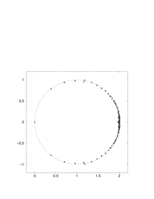
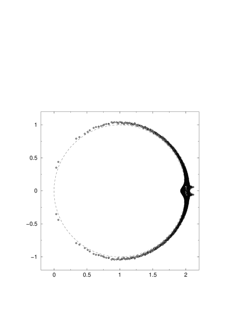
Figure 4.2: The eigenvalue spectrum of the truncated ${\cal D}_{\rm FP}$ in the free case on a $8^{4}$ lattice (top) and the eigenvalue spectrum of ${\cal D}_{\rm par}$ at $\beta=3.0$ on a $4^{4}$ lattice (bottom). The eigenvalues in the free case are highly degenerate and therefore it seems that there are less eigenvalues on the larger lattice than on the small lattice, which is however not true. The figures show clearly, that the GW relation is broken to a lesser extent in the free than in the interacting case; although the eigenvalues in the interacting case are still close to the circle.

In Figure 4.3 we show the physical branch, i.e. the small eigenvalue part, of eigenvalue spectrum of our parametrization II for a minimized $\beta=3.0$ configuration on a $10^{4}$ lattice. The eigenvalues lie very close to the circle. Performing a RGT, the eigenvalue spectrum of the resulting Dirac operator III on the corresponding $5^{4}$ lattice is roughly of the same quality, as the spectrum on the minimized configuration. This shows that the Dirac operator, which we approximate in the last step of the parametrization procedure, has very good chiral properties. In comparison we show the eigenvalue spectrum of the final parametrization IV on the same $5^{4}$ configuration. In this spectrum the alignment of eigenvalues to the circle is clearly inferior to the one of the blocked operator, showing the difficulty of parametrizing $\operatorname{\textfrak{D}_{\rm FP}}$ on rough QCD configurations. But, one has to keep in mind that the final parametrization only has a very small additive mass renormalization and compared to the Wilson Dirac operator, which is shown in the lower part of this figure, the fluctuations of the small (real) modes are reduced considerably.

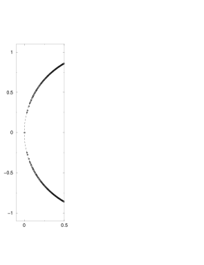
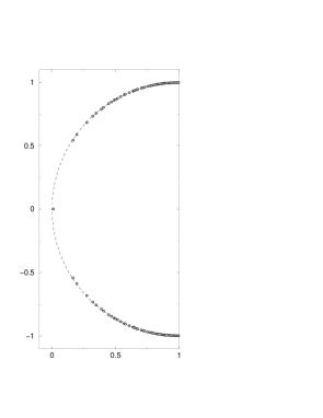
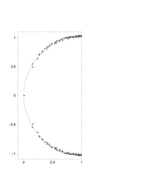
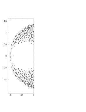
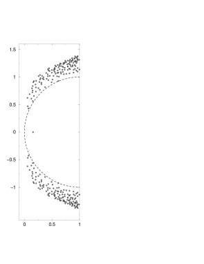
Figure 4.3: Top row: In these figures the physical branch of the eigenvalue spectra on a minimized $10^{4}$ configuration and the corresponding coarse $5^{4}$ configuration at $\beta=3.0$ are shown. The eigenvalues on the minimized configuration (left), which are calculated with operator II, are clearly aligned to the GW circle, which is also the case for the blocked operator III (middle). The alignment of the eigenvalues of the final parametrization IV (right) is clearly worse than the one of the blocked operator III. However, essential features like the small additive mass renormalization are conserved. Bottom row: The eigenvalue spectrum of the Wilson Dirac operator on the same $5^{4}$ configuration at $\beta=3.0$ is shown without (left) and with RG smearing (right). The additive mass renormalization, which is roughly 1.2 and 0.6, respectively, is removed for this comparison. The fluctuations of the small (real) modes are clearly larger than for $\operatorname{{\cal D}_{\rm par}}$; however, one has to be aware that it is only meaningful to compare the fluctuations close to the origin, because the spectrum of a Dirac operator satisfying the GW relation with a general R does not necessarily lie on a circle (see Section 1.2.2).

The eigenvalue spectrum of $\operatorname{\textfrak{D}_{\rm par}}$ does not lie on a circle (see Section 1.2.2) and therefore can not as easily be used to get an impression of the amount of the breaking of chiral symmetry as the eigenvalue spectrum of $\operatorname{{\cal D}_{\rm par}}$. But, because $\operatorname{\textfrak{D}_{\rm par}}$ is the fundamental operator in the parametrization procedure, we show its eigenvalue spectrum on $8^{4}$ lattice in the free case, where the eigenvalues are highly degenerate, and on a $4^{4}$ lattice in the interacting case at $\beta=3.0$ in Figure 4.4.

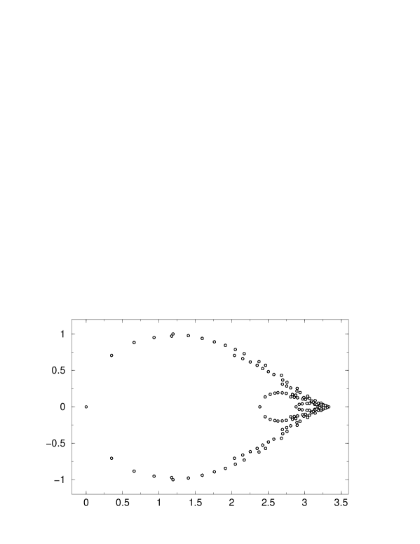
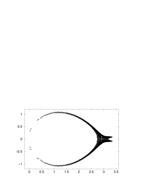
Figure 4.4: Eigenvalue spectrum of the truncated $\operatorname{\textfrak{D}_{\rm FP}}$ in the free case on a $8^{4}$ lattice (top) and the eigenvalue spectrum the production run $\operatorname{\textfrak{D}_{\rm par}}$ at $\beta=3.0$ on a $4^{4}$ lattice (bottom). This figure shows clearly that an operator which satisfies (approximately) the GW relation with $R$ not proportional to $1$ does not lie on a circle (see Section 1.2.2). Notice that the eigenvalues in the free case are highly degenerate.

4.2.2 Breaking of the Ginsparg-Wilson Relation

The FP Dirac operator has an exact chiral symmetry on the lattice. The parametrization $\operatorname{\textfrak{D}_{\rm par}}$, however, satisfies the GW relation no longer exactly. In order to quantify the degree to which it breaks the GW relation, we use the following measure, which is also used in the literature [119, 120]

$$\Delta_{\rm GW}=\big{\langle}||({\cal D}_{\rm par}+{\cal D^{\dagger}_{\rm par}}-{\cal D}^{\dagger}_{\rm par}{\cal D}_{\rm par})v||\big{\rangle}\,,$$ (4.1)

where $v$ is a normalized random vector. The brackets denote the expectation value and $||v||$ is the usual vector norm. Table 4.1 compares $\Delta_{\rm GW}$ of the Dirac operators I-IV. Let us give a few comments to this table: $\Delta_{\rm GW}$ is smaller by one order of magnitude in the free case (operator I) than for the production run parametrization (IV), whereas the parametrization on the minimized configurations (II) performs only slightly worse than the free parametrization on trivial configurations (I). The blocked operator (III) is better than the parametrization on the minimized configurations (II) and almost reaches the same quality as the free parametrization (I). The increase in the breaking of the GW relation with decreasing $\beta$ (i.e. increasing lattice spacing) is as expected. The fluctuations of $\Delta_{\rm GW}$ for different vectors and configurations are very small and finally, $\Delta_{\rm GW}$ does not show any dependence on the lattice size, as expected.

Type	$\beta$	$5^{4}$	$8^{4}$	$10^{4}$
I	free	0.0293(1)	0.0294(1)	0.0294(1)
II	min. 3.4	-	-	0.0525(1)
	min. 3.2	-	-	0.0530(1)
	min. 3.0	-	-	0.0553(1)
	min. 2.7	-	-	0.0604(1)
III	3.4	0.0298(1)	-	-
	3.0	0.0308(1)	-	-
	2.7	0.0339(3)	-	-
IV	3.4	0.1782(2)	0.1779(2)	0.1783(1)
	3.2	0.1885(2)	0.1938(3)	0.1947(1)
	3.0	0.2017(2)	0.2176(4)	0.2172(1)
	2.7	0.2819(2)	0.2816(3)	0.2811(1)

Table 4.1: The breaking of the GW relation $\Delta_{\rm GW}$, as defined in eq. (4.1), is shown for the different types of Dirac operators defined at the beginning of this section. The statistical error is given in the brackets.

4.2.3 Breaking of Normality

A Dirac operator satisfying the GW relation is normal with respect to $R$, which means

$$\operatorname{\textfrak{D}}^{\dagger}R\operatorname{\textfrak{D}}=\operatorname{\textfrak{D}}R\operatorname{\textfrak{D}}^{\dagger}\quad\text{and}\quad{\cal D}{\cal D}^{\dagger}={\cal D}^{\dagger}{\cal D}\,,$$ (4.2)

respectively. Hence, ${\cal D}$ and ${\cal D}^{\dagger}$ are commuting, which implies that the eigenvectors of ${\cal D}$ are also eigenvectors of ${\cal D}^{\dagger}$. A further consequence is that $[{\cal D},\gamma_{5}]=0$ in the subspace of the real eigenmodes and therefore the real eigenmodes of a $\gamma_{5}$-hermitian ${\cal D}$ have definite chirality. Thus, the magnitude of the breaking of normality indicates to what extent e.g. the zero modes are chiral. We measure the non-normality of a Dirac operator $D$ by

$$\Delta_{\rm n}=\big{\langle}||(DD^{\dagger}-D^{\dagger}D)v||\big{\rangle}\,,$$ (4.3)

where $v$ is a normalized random vector. Table 4.2 shows $\Delta_{\rm n}$ for the Dirac operators II-IV. The free case is not indicated, since free Dirac operators are normal. The blocked operator (III) performs slightly worse than the parametrization on the minimized configurations (II), the difference is however very small. The fluctuations of $\Delta_{\rm n}$ for different vectors and configurations are again very small. Finally, $\Delta_{\rm n}$ does not show any dependence on the lattice size, while the dependence on the lattice spacing is again as expected, i.e. the larger the lattice spacing, the larger the breaking of normality.

Type	$\beta$	$5^{4}$	$8^{4}$	$10^{4}$
II	min. 3.4	-	-	0.0196(1)
	min. 3.2	-	-	0.0199(1)
	min. 3.0	-	-	0.0210(1)
	min. 2.7	-	-	0.0235(1)
III	3.4	0.0223(2)	-	-
	3.0	0.0251(2)	-	-
	2.7	0.0312(5)	-	-
IV	3.4	0.0946(2)	0.0950(1)	0.0952(1)
	3.2	0.1027(4)	0.1043(2)	0.1050(1)
	3.0	0.1163(6)	0.1197(2)	0.1196(1)
	2.7	0.1663(10)	0.1662(3)	0.1680(2)

Table 4.2: The breaking of the normality $\Delta_{\rm n}$, as defined in eq. (4.3), is shown for the different types of Dirac operators defined at the beginning of this section.

4.2.4 Eigenvalues of $A^{\dagger}A$

The GW relation eq. (1.20) is equivalent to

$$A^{\dagger}A=1,\hskip 14.22636ptA=1-{\cal D},$$ (4.4)

i.e. that $A$ is a unitary operator. Hence, the breaking of the GW relation is signaled by the occurrence of $A^{\dagger}A$ eigenvalues deviating from 1. In Figure 4.5 we show the density of the $A^{\dagger}A$ eigenvalues for $\operatorname{{\cal D}_{\rm par}}$ at $\beta=3.0$ on a $4^{4}$ lattice. The eigenvalues are distributed between 0.5 and 1.5 with a well-defined peak at 1. For larger physical volumes the distribution typically will have longer tails, which eventually leads to the occurrence of very small $A^{\dagger}A$ eigenvalues.

The ratio of the smallest $\lambda_{\rm min}$ to the largest eigenvalue $\lambda_{\rm max}$ of $A^{\dagger}A$ is related to the asymptotic convergence of approximations to the overlap construction [33]. Hence, this ratio can be used to indicate how expensive the overlap construction is approximately for a certain Dirac operator and gauge action. In Figure 4.6, we plot the 50 smallest eigenvalues of $A^{\dagger}A$ divided by the largest eigenvalue of $A^{\dagger}A$ for $5$ different gauge configurations at gauge coupling $\beta=3.0$ and $\beta=3.5$, respectively. We see that the $A^{\dagger}A$ eigenvalues are much closer to 1 for $\operatorname{{\cal D}_{\rm par}}$ than for $D_{W}$ at both gauge couplings. At this point it should be mentioned that relatively to $D_{W}$ the calculation of the $A^{\dagger}A$ eigenvalues, which is an important ingredient in the numerical implementation of the overlap Dirac operator (see Chapter 5), is by far less expensive for $\operatorname{{\cal D}_{\rm par}}$ than one would naively think. Because $\operatorname{{\cal D}_{\rm par}}$ is substantially closer to be a normal operator and because the $A^{\dagger}A$ eigenvalue spectrum is less dense at the lower edge than for the Wilson operator, the Arnoldi and the Ritz functional method find the eigenvalues with considerably less matrix vector multiplications. The difference is particularly large between $D_{W}$ on unsmeared configurations and $\operatorname{{\cal D}_{\rm par}}$, as shown in Table 4.3, where the number of operator times vector products is given for the Arnoldi method. At the upper edge of the spectrum the difference is much smaller and amounts to roughly 200 matrix vector multiplications for $\operatorname{{\cal D}_{\rm par}}$ and 800 for $D_{W}$, independent of smearing.

Let us finally remark that one might try to use the Chebyshev acceleration technique described in [121] to map the low-lying part of the $A^{\dagger}A$ eigenvalue spectrum onto a larger interval, which in certain cases speeds up the calculation of the eigenvalues and eigenvectors [122]. It would be very interesting to know how $\operatorname{{\cal D}_{\rm par}}$ and $D_{W}$, respectively, can profit from this technique for the calculation of the low-lying $A^{\dagger}A$ eigenvalues.

$\beta$	3.0	3.5
$D_{W}$	16130(212)	17174(154)
$D_{W}^{S}$	6176(212)	8726(122)
${\cal D}_{\rm par}$	682(18)	944(50)

Table 4.3: The average number of Dirac operator times vector multiplications to find the $50$ lowest $A^{\dagger}A$ eigenvalues for ${\cal D}_{\rm par}$ and the Wilson Dirac operator on smeared ($D_{W}^{S}$) and unsmeared ($D_{W}$) gauge configurations. This table shows that calculations using ${\cal D}_{\rm par}$ do not necessarily have to be as expensive as one would naively think, because the large difference in the number of matrix vector multiplications between $\operatorname{{\cal D}_{\rm par}}$ and $D_{W}$ almost compensates for the overhead of $\operatorname{{\cal D}_{\rm par}}$ in one matrix vector multiplication.

Figure 4.5: Density $\rho(\lambda)$ of the $A^{\dagger}A$ eigenvalues of $\operatorname{{\cal D}_{\rm par}}$ on a $4^{4}$ configuration at $\beta=3.0$. On larger volumes the probability of small $A^{\dagger}A$ eigenvalues increases, which makes that a tail on the left hand side of the peak develops. At the upper edge of the spectrum, however, the structure of the distribution does not change significantly at larger volumes.

\psfrag{FP}{\footnotesize$\operatorname{{\cal D}_{\rm par}}$}\psfrag{DWS}{\footnotesize$D_{W}^{S}$}\psfrag{DW}{\footnotesize$D_{W}$}\includegraphics[width=312.9803pt]{adaga_b300_n12}

\psfrag{FP}{\footnotesize$\operatorname{{\cal D}_{\rm par}}$}\psfrag{DWS}{\footnotesize$D_{W}^{S}$}\psfrag{DW}{\footnotesize$D_{W}$}\includegraphics[width=312.9803pt]{adaga_b350_n12}

Figure 4.6: The ratio of the 50 smallest $A^{\dagger}A$ eigenvalues to the largest $A^{\dagger}A$ eigenvalue on 5 different $12^{4}$ configurations at $\beta=3.0$ (top) and $\beta=3.5$ (bottom) is shown for $\operatorname{{\cal D}_{\rm par}}$, $D_{W}^{S}$ and $D_{W}$. As expected this ratio is clearly closer to 1 for $\operatorname{{\cal D}_{\rm par}}$ than for $D_{W}$. Notice that the legend is valid for both figures.

4.2.5 Index Theorem

For GW fermions the Atiyah-Singer index theorem from eq. (1.27) holds. Recalling the previous discussion about the distribution of the $A^{\dagger}A$ eigenvalues we can not expect the index theorem to hold for $\operatorname{{\cal D}_{\rm par}}$ because it can be rewritten as follows

$${\rm index}(\operatorname{{\cal D}})=\frac{1}{2}\operatorname{Tr}(\gamma_{5}\operatorname{{\cal D}})=-\frac{1}{2}\operatorname{Tr}(\gamma_{5}(1-\operatorname{{\cal D}}))=-\frac{1}{2}\operatorname{Tr}(\gamma_{5}A),$$ (4.5)

where we use $\operatorname{Tr}\gamma_{5}=0$. Hence, small eigenvalues of $\gamma_{5}A$ and, in particular, an unsymmetric distribution of $\gamma_{5}A$ eigenvalues tend to destroy the correspondence given by the index theorem. We will discuss our definition of the index of $\operatorname{{\cal D}_{\rm par}}$, which does not satisfy the GW relation exactly, and therefore has no exact zero modes with definite chirality in Section 6.1.1. In Figure 4.7 we see that the relation is indeed distorted heavily for the production run parametrization. The definition of the index using the trace leads to a result which on average is too large by a factor of $3.16$. In Figure 4.8 we compare the index of $\operatorname{{\cal D}_{\rm par}}$ with the index of the corresponding overlap operator constructed from $\operatorname{{\cal D}_{\rm par}}$ (see Chapter 5), which has a very precise chiral symmetry. We see that the index of the Dirac operator defined through the low-lying real eigenmodes and their chirality is a much more stable quantity than the index defined through $1/2\operatorname{Tr}(\gamma_{5}\operatorname{{\cal D}_{\rm par}})$, because it coincides with the index of the overlap Dirac operator in most of the cases. We will use this observation in Chapter 6, where we calculate the topological susceptibility.

In contrast to the production run parametrization the trace definition of the index works well on the minimized configurations when the corresponding Dirac operator is used (definition II), despite the fact that the wrong sign in the normalization condition for the topological charge density was used in the parametrization (see Section 3.2.2). This means that the linear polynomials in the couplings really could straighten out the error in the normalization condition and therefore we can also conclude that the problems with the trace definition of the index, we see in the production run parametrization, are due to other problems. Maybe an even richer parametrization for the pseudoscalar part is needed to give an accurate description of $1/2\operatorname{Tr}(\gamma_{5}\operatorname{{\cal D}_{\rm par}})$ on configurations used in simulations.

Figure 4.7: The correlation between the index of $\operatorname{{\cal D}_{\rm par}}$ and $1/2\operatorname{Tr}(\gamma_{5}\operatorname{{\cal D}_{\rm par}})$ is shown for 50 $8^{4}$ configurations at $\beta=3.0$. One can see that a certain correlation between the two quantities remains, but the index theorem clearly does not hold for the parametrized operator. The definition with the trace gives a result which on average is too large by a factor of $3.16$ as indicated by the dashed line. The solid line shows, where the points actually should lie if the index theorem would be satisfied.

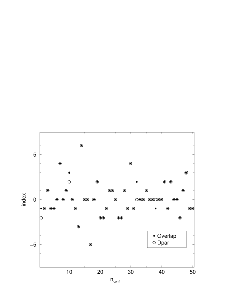
Figure 4.8: The correlation between the index of $\operatorname{{\cal D}_{\rm par}}$ and the corresponding overlap construction with $\operatorname{{\cal D}_{\rm par}}$ is shown for 50 $8^{4}$ configurations at $\beta=3.0$. One can see that the value of the index defined by $\operatorname{{\cal D}_{\rm par}}$ coincides on most of the configurations with the overlap definition.

4.2.6 Residual Additive Mass Renormalization and Fluctuations of the Low-Lying Modes

Another very important property of a Dirac operator satisfying the GW relation is the absence of an additive mass renormalization and related to this, the protection against exceptional configurations at non-zero quark mass. This means that the pions get massless if the bare quark mass is zero, making that no fine tuning of parameters is needed to reach the chiral limit [39]. Even more important is the fact that there are no fluctuations in the low-lying modes of the Dirac operator that make the simulation of (quenched) QCD in (or at least near) the region of the physical up and down quark mass impossible. For $\operatorname{\textfrak{D}_{\rm par}}$ there is a residual additive mass renormalization and there are fluctuations in the small eigenmodes that do not allow to simulate at an arbitrarily small quark mass, but the situation is definitely improved compared to the Wilson Dirac operator, where the fluctuations in the low-lying modes make the simulations difficult at a $\pi/\rho$ ratio of 0.5 to 0.4, depending on the lattice spacing and the volume [123, 124]. The clover improved Wilson Dirac operator is even worse in this respect, i.e. that the low-lying eigenvalues fluctuate even more. Exceptional configurations were already found at a $\pi/\rho$ ratio of $0.54$ at a lattice spacing of $0.1\,{\rm fm}$ [125]. Finally, the situation does not seem to improve as much as expected in the case of full QCD simulations [126]. In our hadron spectroscopy study, which is described in detail in [65], we were able to simulate down to a $\pi/\rho$ ratio of 0.28, which corresponds to a quark mass of roughly 10 MeV in the $\overline{\rm MS}$ scheme at $\mu=2\,{\rm GeV}$; notably, without facing the problem of exceptional configurations in an ensemble of 200 $16^{3}\times 32$ configurations at a lattice spacing $a=0.155\,{\rm fm}$ ($\beta=3.0$). From this study we can extract the residual additive quark mass renormalization $a\Delta_{\rm m}$ and an upper limit for the minimal bare quark mass $am_{\rm min}$ that is needed to prevent from the appearance of exceptional configurations. The results are given in Table 4.4 and show that the additive mass renormalization and the fluctuations of the low-lying modes are small. The result on the largest physical volume at $\beta=3.0$ is the most impressive as the bare mass can be chosen to be very small.

$\beta$	$a\Delta_{\rm m}$	$am_{\rm min}$
3.0	-0.0006(4)	0.013
3.4	-0.0180(4)	0.029
3.7	-0.0194(4)	0.0235

Table 4.4: The additive mass renormalization and the smallest bare mass used in the hadron spectroscopy simulations in [65]. The values at $\beta=3.0$ are from a larger physical volume and therefore it is possible to go to even smaller quark masses.

4.3 Scaling Properties of the Parametrized FP Dirac Operator

The FP Dirac operator is expected to have small scaling violations. This is a crucial property that allows one to simulate at larger lattice spacings with only very small distortions of the continuum physics. We do not cover the scaling properties of $\operatorname{\textfrak{D}_{\rm par}}$ as detailed as the chiral properties; the reason for this is not the significance of scaling properties, but simply the fact that it is computationally much more expensive to get information on scaling. This explains why there is not much data on scaling properties, yet.

Presently, our only source of data on the scaling behaviour of $\operatorname{\textfrak{D}_{\rm par}}$ is the hadron mass spectroscopy measurement described in [65]. The simulations are performed at $3$ different lattice spacings. The extent of the lattice is chosen such that all $3$ measurements are done in the same physical volume with a spatial extent of $L\approx 1.22\,{\rm fm}$, in order to allow for a continuum extrapolation. This volume is rather small, which makes that the masses of the particles (especially of the baryons) are distorted by finite volume effects [127]. But because the finite volume distortions are physical effects, the data is nevertheless suited for a scaling analysis, even though uncertainties in the scale determination lead to larger uncertainties in the scaling analysis than for larger volumes, where the dependence of the particle masses on the volume is negligible. The data at $\beta=3.0,3.4$ and $3.7$ for the vector meson, the decuplet and octet baryons is shown in Figure 4.9. It indicates a remaining ${\cal O}(a^{2})$ scaling violation. However, a more careful analysis is needed, because there are several sources of systematic errors. Most significantly is probably the uncertainty in the scale, as the interpolating formula the Sommer scale $r_{0}$ in [95, 96] covers the range $\beta=2.361,\ldots,3.4$ and therefore an extrapolation for the value at $\beta=3.7$ has been used. Furthermore, this scale determination has a systematic error which is not accounted for in Figure 4.9. The data is not accurate enough to completely exclude ${\cal O}(a)$ scaling violations – which are definitely not present in the hadron spectrum for a GW Dirac operator [52] – but, if there are remaining ${\cal O}(a)$ scaling violations, then they are very small. This is actually supported by the fact that also the energy-momentum dispersion relation for the pseudoscalar and the vector meson do not show any visible cut-off effect, as shown in Figure 4.10.

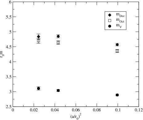
Figure 4.9: Scaling of the hadron masses (vector meson, octet and decuplet baryon) calculated with $\operatorname{\textfrak{D}_{\rm par}}$ at 3 different lattice spacings. The data suggests that the remaining scaling violations are mostly ${\cal O}(a^{2})$ effects and are rather small.

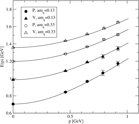
Figure 4.10: Energy-momentum dispersion relation $E(\vec{p})$ for pseudoscalar (P) and vector mesons (V) on the $16^{3}\times 32$ lattice at $\beta=3.0$. The solid lines show the continuum value with $E(0)$ given by the measured mass.

4.4 Discussion

The parametrized FP Dirac operator, which we obtained from the fitting procedure in Chapter 3, is clearly improved in many respects in comparison to the Wilson Dirac operator. It has a relatively small breaking of chiral symmetry that allows to calculate the hadron mass spectrum down to quark masses of roughly 10 MeV in the $\overline{\rm MS}$ scheme at $\mu=2\,{\rm GeV}$. Even though the physical point can not yet be reached with the present parametrization, it is a remarkable progress in comparison to Wilson fermions. Furthermore, it is possible to go to such small quark masses that there is a clear signal for quenched chiral logarithms, even in the data of the pseudoscalar spectroscopy with degenerate quark masses [65]. The comparison of the parametrization with the blocked operator obtained from the RGT shows the limitations of the present parametrization, because the blocked operator has smaller breaking of chiral symmetry. Furthermore, the present parametrization does not satisfy the index theorem. But one should keep in mind that the topological charge density is a quantity which is of small order and in the present parametrization no particular effort was undertaken to make the fitting procedure more sensitive to the pseudoscalar contribution and therefore some improvement might be achieved in future parametrizations. The data for the scaling of the hadron masses suggests that the present parametrization leads to remaining cut-off effects which are mainly ${\cal O}(a^{2})$ and as shown in [65] the cut-off effects are on the order of various other ${\cal O}(a)$ improved Dirac operators. As discussed in Section 4.3, the sources of systematic errors are too large to make a clear statement on the size of the ${\cal O}(a^{2})$ scaling violations, apart from the fact that they are rather small. The data, however, indicates that order ${\cal O}(a)$ cut-off effects are very small, as one can see no sign of their presence. These statements about the small scaling violations are supported by the fact that the energy-momentum dispersion relation for the pseudoscalar and the vector meson do not show any visible cut-off effect.

Chapter 5 Overlap Construction with the Parametrized FP Dirac Operator

One of the very important properties of $\operatorname{\textfrak{D}_{\rm FP}}$ is its exact chiral symmetry on the lattice [128]. Unfortunately, this exact symmetry gets lost through the parametrization. As expected, the violation of chiral symmetry is much smaller for $\operatorname{\textfrak{D}_{\rm par}}$ than for Wilson fermions. In addition, Neuberger’s overlap construction [40, 41] gives a recipe, how a Dirac operator that respects chiral symmetry on the lattice can be constructed from any Dirac operator that has no doublers in the continuum limit and is local [129]. In numerical simulations approximations to Neuberger’s construction can be used to obtain Dirac operators whose violations of chiral symmetry are, in principle, below an arbitrarily chosen limit. Very precise chiral symmetry is required for some measurements, such as the chiral condensate [130]. However, the decision to what extent chiral symmetry is needed for a particular calculation has to be taken from case to case, since (approximately) chiral actions are computationally very expensive [120, 98].

In this chapter we first discuss Neuberger’s overlap formula and then, in particular, the properties of the overlap construction with $\operatorname{\textfrak{D}_{\rm par}}$ and $R_{\rm par}$. The actual construction with $R\neq 1/2$ is numerically somewhat more involved than the standard case $R=1/2$ and we give the technical details in Appendix D. Below, we explain the details of the Legendre expansion of the operator $(A^{\dagger}A)^{-1/2}$ in the overlap formula, because in our simulations with the overlap we exclusively use this type of approximation. We present results on the properties of the overlap construction with $\operatorname{\textfrak{D}_{\rm par}}$ and $R_{\rm par}$ and make some comparisons to the standard overlap construction with the Wilson Dirac operator. Finally, we conclude with a remark on scaling properties of the overlap construction with $\operatorname{{\cal D}_{\rm par}}$.

5.1 General Overlap Construction

The overlap formula in terms of a Dirac operator $D$ and the local gauge operator $R$ from the GW relation eq. (1.1) in the massless case is given by

$${\cal D} =1-A(A^{\dagger}A)^{-1/2}=1-\gamma_{5}\epsilon(\gamma_{5}A)$$ (5.1)

with

$$A =1+s-(2R)^{1/2}D(2R)^{1/2}\,,$$ (5.2)

where $\epsilon(\gamma_{5}A)$ is the matrix sign function of the operator $\gamma_{5}A$. The real parameter $s$ is important for the overlap construction with the Wilson Dirac operator, where it can be used to optimize e.g. the localization range or the convergence rate of an approximation [131]. In connection with the overlap with $\operatorname{{\cal D}_{\rm par}}$ the parameter $s$ does not play a rôle, because there is no need to shift the $A^{\dagger}A$ eigenvalues, since they are already centered around 1 as shown in Figure 4.5. It is easy to see that $\operatorname{{\cal D}}$ satisfies the GW relation. More generally, it possible to define

$$\operatorname{\textfrak{D}}=(2R)^{-1/2}(1-A(A^{\dagger}A)^{-1/2})(2R)^{-1/2}=(2R)^{-1/2}(1-\gamma_{5}\epsilon(\gamma_{5}A))(2R)^{-1/2}\,,$$ (5.3)

where the operator $A$ is again as defined in eq. (5.2), such that $\operatorname{\textfrak{D}}$ satisfies the GW relation with a general $R$. The inverse square root of the hermitian operator $A^{\dagger}A$ or the matrix sign function of $\gamma_{5}A$ are the objects that cause all the trouble in the overlap formula. They have to be approximated in a certain way, because a full decomposition of these operators into their eigenmodes is computationally not feasible, even for modest lattice sizes. In the last $5$ years many different approximation schemes have been worked out and applied to this problem. One of the main directions of approximation schemes deals with polynomial expansions, like Legendre [131], Gegenbauer [132] or Chebyshev polynomials [120], while the other main direction is concerned with rational approximations, like the Remes method [133], the polar decomposition [134] or the Zolotarev polynomials [135, 98]. Furthermore, there are also direct Krylow subspace methods used to approximate the matrix sign function [136, 137] and some attempts to formulate algorithms in a 5-dimensional space in order to avoid nested Krylow methods, which are used in the rational approximations. Such 5-dimensional approximations have a close relation to the domain-wall fermion approach [138, 139].

It is useful to introduce the mass term of a Dirac operator satisfying the GW relation in a particular way, namely

$${\cal D}(m)=\Big{(}1-\frac{m}{2}\Big{)}{\cal D}(0)+m$$ (5.4)

and

$$\operatorname{\textfrak{D}}(m)=\Big{(}1-\frac{m}{2}\Big{)}\operatorname{\textfrak{D}}(0)+m(2R)^{-1}\,,$$ (5.5)

respectively. With this definition the scalar density $S$ is defined as follows

$$S=\bar{\psi}\Big{(}1-\frac{1}{2}{\cal D}(0)\Big{)}\psi$$ (5.6)

and

$$S=\bar{\psi}\Big{(}(2R)^{-1}-\frac{1}{2}\operatorname{\textfrak{D}}(0)\Big{)}\psi$$ (5.7)

for the general case. Defined this way the scalar density transforms under chiral transformations like the corresponding continuum density [140]. This implies that this density, which is a dim=3 operator, is ${\cal O}(a)$ improved, since it does not mix with any dim=4 operator. A detailed discussion of these densities and the construction of chiral covariant currents, which are also ${\cal O}(a)$ improved, is given in [140].

Our choice of the Legendre expansion might surprise a little bit when consulting the literature about the different approximations, because the Legendre expansion does not figure among the most efficient schemes [98]. However, the discussion of these approximations is almost entirely concentrated on the overlap construction with Wilson fermions, which is completely different due to the fact that the operator $A^{\dagger}A$ deviates much more from $1$ than in the case of $\operatorname{{\cal D}_{\rm par}}$ (see Figure 4.6), and therefore high order polynomials have to be used in the approximations. On the contrary, $\operatorname{{\cal D}_{\rm par}}$ is already quite close to satisfy the GW relation and therefore low order polynomial approximations can be used to approximate e.g. the operator $(A^{\dagger}A)^{-1/2}$. For low order approximations, however, the difference between the different polynomial approximations is much less pronounced than at high orders. In fact, our experiments with the Chebyshev expansion didn’t show a visible advantage for the Chebyshev expansion at polynomial orders of $\leq 4$, but clearly more precise studies are needed to clarify this issue.

5.1.1 Legendre Expansion

Following the original work [131], we give a short description of Legendre expansion of the operator $(A^{\dagger}A)^{-1/2}$.

In order to ensure convergence of the Legendre expansion we assume that the bounds

$$u\leq\langle\psi|A^{\dagger}A|\psi\rangle\leq v$$ (5.8)

hold for some strictly positive constants $u<v$ and arbitrary normalized states $|\psi\rangle$.

The Legendre polynomials $P_{k}(z)$ may be defined through the generating functional

$$(1-2tz+t^{2})^{-1/2}=\sum_{k=0}^{\infty}t^{k}P_{k}(z)\,.$$ (5.9)

Usually $z$ is taken to be a number, but (5.9) remains meaningful if we substitute

$$z=\frac{v+u-2A^{\dagger}A}{v-u}\,.$$ (5.10)

The expansion (5.9) is convergent for all $t$ satisfying $|t|<1$.

Introducing the parameter $\theta$ through

$$\cosh\theta=\frac{v+u}{v-u}\,,\qquad\theta>0\,,$$ (5.11)

and $t=e^{-\theta}$ (5.9) takes the form

$$(A^{\dagger}A)^{-1/2}=\kappa\sum_{k=0}^{\infty}t^{k}P_{k}(z)\,,\qquad\kappa=\sqrt{\frac{4t}{v-u}}\,,$$ (5.12)

since $1-2tz+t^{2}$ is proportional to $A^{\dagger}A$ for this choice of $t$. In practical applications the sum in (5.12) will be truncated after a finite number of terms and this then defines the Legendre expansion of the overlap operator to a certain order $N$, which we denote by ${\cal D}^{(N)}$ or ${\operatorname{\textfrak{D}}}^{(N)}$, respectively.

5.1.2 Exact Projection of $A^{\dagger}A$ Eigenvalues

For large volumes and small values of $\beta$ the eigenvalues of $A^{\dagger}A$ tend to scatter further away from $1$, even for $\operatorname{{\cal D}_{\rm par}}$. This eventually leads to big problems in the numerical expansions used for the inverse square root or the sign function, because the parameter $c$ governing the asymptotic convergence of these expansions is [33]

$$||{\cal D}^{(N)}-{\cal D}||=e^{-cN},\quad c=\sqrt{\frac{\lambda_{\rm min}}{\lambda_{\rm max}}}\,,$$ (5.13)

where $\lambda_{\rm min}$ is the smallest eigenvalue of $A^{\dagger}A$ and $\lambda_{\rm max}$ the largest. Because the distribution of the eigenmodes of $A^{\dagger}A$ is typically not very dense at the lower edge of the spectrum, one can use exact projection methods to decrease the condition number $c$ substantially. The same is not true for the upper edge of the spectrum of $A^{\dagger}A$, because the modes lie much denser there. Let us specify what we mean by the exact projection of the $n$ eigenmodes $|\psi_{i}\rangle$ of $\gamma_{5}A$ with the eigenvalues $\lambda_{i}$ of smallest modulus:

$$(A^{\dagger}A)^{-1/2}=\sum_{i=1}^{n}\frac{1}{|\lambda_{i}|}|\psi_{i}\rangle\langle\psi_{i}|+{\cal P}^{n}_{\perp}\,{\rm App}\big{[}(A^{\dagger}A)^{-1/2}\big{]}{\cal P}^{n}_{\perp},$$ (5.14)

for the square root and

$$\epsilon(\gamma_{5}A)=\sum_{i=1}^{n}\epsilon(\lambda_{i})|\psi_{i}\rangle\langle\psi_{i}|+{\cal P}^{n}_{\perp}\,{\rm App}[\epsilon(\gamma_{5}A)]{\cal P}^{n}_{\perp}$$ (5.15)

for the matrix sign function, where the projection to the subspace orthogonal to the lowest $$n$$ eigenmodes is defined by

$${\cal P}^{n}_{\perp}=1-\sum_{i=1}^{n}|\psi_{i}\rangle\langle\psi_{i}|$$ (5.16)

and where ${\rm App}$ stands for one of the possible expansions which may be used in practice. The calculation of the $A^{\dagger}A$ eigenvalues and eigenmodes can be performed e.g. with the Ritz functional [104, 105] or the implicitly restarted Arnoldi method [113, 114]. In our overlap studies we mainly use the Arnoldi method to calculate the eigenmodes, because it showed to be efficient in the search of rather large numbers ($\leq 200$) of small $A^{\dagger}A$ eigenvectors.

5.2 Properties of the Overlap with FP Kernel

In the following discussion of the properties of the overlap construction with $\operatorname{{\cal D}_{\rm par}}$ as kernel we focus on two topics: the locality of the resulting operator and the dependence of the remaining breaking of chiral symmetry on the precision of the approximation.

5.2.1 Locality

A lattice action must be local for the continuum results to be universal, i.e. independent of the details of the lattice action. Locality means that fields at large separations $r=|y-x|\gg 1$ have an exponentially small coupling $\rho(r)$, i.e. $\rho(r)\sim\exp(-\nu r)$ with $\nu={\cal O}(1)$. Optimizing the locality is essential so that e.g. the exponential fall-off of correlation functions can be separated from direct couplings in the lattice action even on coarse lattices. The locality of a lattice Dirac operator can be measured by

$$f_{p}(r)={\rm max}\{||Dv||,||y-x||_{p}=r\},$$ (5.17)

where $v$ is a vector with point source at $x$ and $||v||_{p}=(\sum_{i=1,n}|v_{i}|^{p})^{1/p}$ is the vector norm. We use the usual vector norm (p=2) and the taxi driver norm (p=1) to discuss the data. These two norms are also the most common choices in the literature [131, 116]. In Figure 5.1, we present the locality measured by the expectation value of the normalized function $f_{2}(r)/f_{2}(0)$ of the overlap construction with $\operatorname{{\cal D}_{\rm par}}$ and the Wilson Dirac operator on smeared ($D_{W}^{S}$) and unsmeared configurations ($D_{W}$) at $\beta=3.0$ and $\beta=3.5$ on $12^{4}$ lattices. We use a Legendre expansion of order $250$ for the Wilson overlap and order $25$ for the overlap with $\operatorname{{\cal D}_{\rm par}}$ and project out the 50 lowest $A^{\dagger}A$ eigenmodes to make sure that the deviations from the exact overlap Dirac operator are smaller than the couplings at $r/a=12$. The locality for the Wilson overlap is optimized by adjusting the parameter $s$ in eq. (5.1). The overlap construction with $\operatorname{{\cal D}_{\rm par}}$ is clearly more local than the Wilson overlap, independent of smearing. While the exponential fall-off of the $\operatorname{{\cal D}_{\rm par}}$ overlap stays the same on both gauge couplings, this is not the case with the Wilson overlap, whose locality gets slightly worse with stronger coupling. In Table 5.1 we list the exponents $\nu$ obtained from an exponential fit to the expectation value of $f_{p}(r)$

$$\langle f_{p}(r)\rangle\propto e^{-\nu r/a}\,,$$ (5.18)

where $r/a>13$ for $p=1$ and $r/a>7$ for $p=2$. The results in Table 5.1 show that with the overlap with $\operatorname{{\cal D}_{\rm par}}$ one can investigate masses up to $ma\approx 1.5$ in spectroscopy calculations. Finally, the overlap construction from eq. (5.3) with $\operatorname{\textfrak{D}_{\rm par}}$ and $R_{\rm par}$ has the same exponential fall-off as the construction from eq. (5.1).

$\beta$	3.5		3.0
p	1	2	1	2
$D_{W}$	0.48(1)	1.14(5)	0.42(1)	0.94(3)
$D_{W}^{S}$	0.58(1)	1.32(5)	0.55(1)	1.22(4)
${\cal D}_{\rm par}$	0.81(2)	1.60(2)	0.82(1)	1.60(2)

Table 5.1: Value of the exponent $\nu$ as defined in eq. (5.18) for the overlap construction from eq. (5.1) with different Dirac operators and for the taxi driver norm (p=1) as well as the usual vector norm (p=2), which gives the locality in terms of physical distances.

\psfrag{FP}{\footnotesize$\operatorname{{\cal D}_{\rm par}}$}\psfrag{DWS}{\footnotesize$D_{W}^{S}$}\psfrag{DW}{\footnotesize$D_{W}$}\includegraphics[width=270.30118pt]{locality_b350}

\psfrag{FP}{\footnotesize$\operatorname{{\cal D}_{\rm par}}$}\psfrag{DWS}{\footnotesize$D_{W}^{S}$}\psfrag{DW}{\footnotesize$D_{W}$}\includegraphics[width=270.30118pt]{locality_b300}

Figure 5.1: Locality of the overlap Dirac operator using $D_{W}$, $D_{W}^{S}$ and $\operatorname{{\cal D}_{\rm par}}$ on $12^{4}$ configurations at $\beta=3.5$ (top) and $\beta=3.0$ (bottom). The overlap construction with $\operatorname{{\cal D}_{\rm par}}$ is clearly more local than the Wilson overlap, independent of smearing. While the exponential fall-off of the $\operatorname{{\cal D}_{\rm par}}$ overlap stays the same at both gauge couplings, this is not the case for the Wilson overlap, whose locality gets worse with stronger coupling.

5.2.2 Chiral Properties

In this section we consider the breaking of chiral symmetry defined through various quantities. We use again the breaking of the GW relation $\Delta_{\rm GW}(N)$ and the breaking of normality $\Delta_{\rm n}(N)$ on normalized random vectors, as defined in eqs. (4.1) and (4.3); however, with the additional dependence on the order $N$ of the Legendre expansion. But first we try to characterize the deviations of the eigenvalues from the GW circle.

The eigenvalue spectrum is suited to show deviations from the GW circle. However, when the GW breaking $\Delta_{\rm GW}$ drops below $\sim 10^{-2}$, it gets difficult to judge the quality of the approximation by eye, which makes it necessary to use a different measure to visualize the deviations from the circle. Hence, we use the fact that if the eigenvalues $\lambda$ of $\operatorname{{\cal D}}$ lie exactly on the GW circle, then the stereographic projection

$$\Lambda=\frac{\lambda}{1-\frac{\lambda}{2}}$$ (5.19)

is purely imaginary. In Figure 5.2, we see that ${\rm Re}(\Lambda)$ falls off exponentially as we increase the polynomial order, showing that the eigenvalues $\lambda$ get closer and closer to the GW circle. The most rapid decrease is at the finest lattice spacing $a\approx 0.10\,{\rm fm}$ ($\beta=3.4$), which is what one expects.

In Figure 5.3 the breaking of the GW relation and the breaking of the normality is shown on $10^{4}$ lattices at $\beta=3.0$, $\beta=3.2$ and $\beta=3.4$. First of all we see that the breaking $\Delta_{\rm GW}(N)$ and $\Delta_{\rm n}(N)$ fall off exponentially as we increase the order $N$ of the Legendre polynomial approximation of $(A^{\dagger}A)^{-1/2}$. Treating the the same number of $A^{\dagger}A$ eigenvalues exactly, the fall-off is clearly the steepest for the smallest lattice spacing ($\beta=3.4$), which is what one expects. When the number of projected $A^{\dagger}A$ eigenvalues, however, is decreased such that the ratio $\lambda_{\rm min}/\lambda_{\rm max}$ is approximately the same on all lattice spacings (this actually corresponds to projecting only the 20 lowest eigenvalues of $A^{\dagger}A$ at $\beta=3.2$ and the 5 lowest at $\beta=3.4$) the approximation is of the same quality to a very high degree. In Table 5.2 we collect the exponents $\mu$ describing the fall-off of $\Delta_{\rm GW}(N)$ with increasing order of the Legendre expansion and compare it to the predicted asymptotic value $c$ from eq. (5.13). Notice that the exponent $\mu$ is clearly larger than the asymptotic value in all cases, which indicates that the regime of asymptotic convergence is by far not reached, making the convergence in the region that is interesting for simulations much faster than in the worst case. But, all the same the value $c$ seems to be in clear correlation with the measured fall-off $\mu$. The results are based on rather low statistics and in order to make the statement more quantitative clearly more statistics is needed.

$\beta$	$\mu$	c
3.4	1.66	0.67
3.2	1.51	0.63
3.0	1.26	0.55

Table 5.2: Value of the exponent $\mu$ giving the exponential fall-off of the breaking of the GW relation in terms of $\Delta_{\rm GW}(N)$ is compared to the asymptotic fall-off given by the condition number $c$, defined in eq. (5.13). The exponential fall-off of $\Delta_{\rm GW}(N)$ is clearly steeper than the asymptotic fall-off, but $c$ is obviously correlated to $\mu$. The data is obtained from $10^{4}$ lattices.

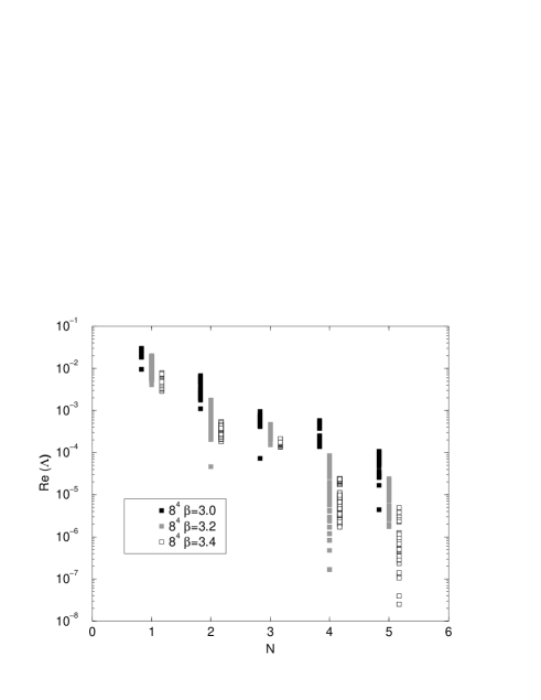
Figure 5.2: Deviation of the ${\cal D}^{(N)}$ eigenvalues from the GW circle defined by the stereographic projection in eq. (5.19).

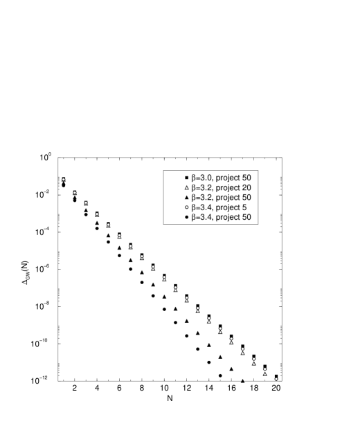
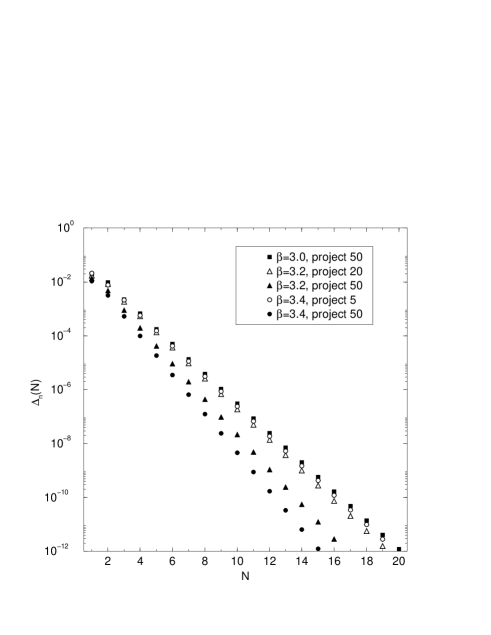
Figure 5.3: Breaking of Ginsparg-Wilson relation $\Delta_{\rm GW}(N)$ (top) and the breaking of normality $\Delta_{\rm n}(N)$(bottom) on $10^{4}$ lattices. Both quantities have almost exactly the same exponential fall-off, even though $\Delta_{\rm n}(N)$ remains slightly smaller for all the orders of the Legendre approximation shown on this figure. The figure also shows that the exponential fall-off is rather governed by the condition number $c$, defined in eq. (5.13), because the exponent is roughly the same for the $3$ different lattice spacings, where the lower boundary of the projected $A^{\dagger}A$ eigenvalues is chosen such that the condition number $c$ is approximately the same.

5.3 A Final Remark

The overlap construction with $\operatorname{{\cal D}_{\rm par}}$ can be looked upon as a tool to cure the breaking of chiral symmetry that remains in the parametrized FP Dirac operator. Clearly, one hopes that the good scaling properties of the FP Dirac operator, which to a certain extent are still present after the parametrization process, are not distorted too much by the overlap construction. In the best case the overlap cures some small remaining ${\cal O}(a)$ cut-off effects in hadron spectroscopy measurements, without creating larger ${\cal O}(a^{2})$ scaling violations. The hadron spectroscopy measurements performed in [65], which do not only contain simulations with $\operatorname{\textfrak{D}_{\rm par}}$, but also include simulations with an order $3$ Legendre polynomial expansion of the overlap Dirac operator from eq. (5.3) with $\operatorname{\textfrak{D}_{\rm par}}$ and $R_{\rm par}$ at a lattice spacing of $0.155\,{\rm fm}$ ($\beta=3.0$), may be interpreted this way. It is, however, very risky to make such a conclusion with so little data. The results on the dependence of the vector meson mass with respect to the pseudoscalar mass show that there are larger discrepancies between the measurements with $\operatorname{\textfrak{D}_{\rm par}}$ and the corresponding overlap construction than one might expect. Furthermore, the energy-momentum relation for the overlap construction indicates cut-off effects. Even though the differences cancel in the Edinburgh plot, the data indicates different cut-off effects for $\operatorname{\textfrak{D}_{\rm par}}$ and the corresponding overlap construction. To conclude this section we compare the physical branch of the eigenvalue spectrum of the blocked Dirac operator obtained from the RGT equations (3.1) and (3.20) (Dirac operator II in the nomenclature of Chapter 4) with the overlap construction with $\operatorname{{\cal D}_{\rm par}}$ in Figure 5.4. It shows that even if the overlap construction shifts the eigenvalues to the circle, there remains a visible difference between the two spectra, which indicates that the cut-off effects for the two Dirac operators might, indeed, be different. The question how large the cut-off effects are for the different Dirac operators discussed in this section has surely to be answered in future studies.

Figure 5.4: The physical branch of the eigenvalue spectra of the blocked Dirac operator (left) and the overlap Dirac operator with $\operatorname{{\cal D}_{\rm par}}$ as kernel (right) are shown. One observes that the eigenvalues of the blocked operator are shifted away slightly more from the origin than the eigenvalues of the overlap Dirac operator. This indicates that, even though the overlap construction cures the remaining breaking of chiral symmetry in $\operatorname{{\cal D}_{\rm par}}$, the overlap Dirac operator with $\operatorname{{\cal D}_{\rm par}}$ might show different cut-off effects than the (approximate) FP Dirac operator, defined through the block transformation in eqs. (3.1) and (3.20). The lines on the figure are shown to make the different locations of the eigenvalues more evident.

Chapter 6 Topological Susceptibility and Local Chirality of Near-Zero Modes

The zero modes as well as the low-lying modes of the Dirac operator have a particularly important influence on several important phenomena of QCD, because their contribution to the quark propagator gets very large in the chiral limit. Topological excitations like instantons might be responsible for the spontaneous breaking of chiral symmetry by building up a non-zero density of eigenvalues at zero in the infinite volume limit; a fact which is encoded in the Banks-Casher relation [141]. Instantons also provide an explanation for the large mass of the $\eta^{\prime}$ particle [142]. Related explanations for the mass of the $\eta^{\prime}$ predict a connection between the quenched topological susceptibility and the mass of the $\eta^{\prime}$ [143, 144].

The question has recently been raised if it is possible to show that the near-zero modes are dominated by instantons or whether instantons are not important to explain the non-perturbative properties of the QCD vacuum.

Answers to questions related to gauge field topology and its influence on the low-lying modes of the fermions living on such a gauge background can be explored within lattice QCD. Lattice Dirac operators which satisfy the GW relation provide an excellent framework to study topological excitations of the QCD vacuum. They allow a definition of the topological charge and the topological charge density on the lattice which is unambiguous in the continuum limit (see Section 1.2.2). Hence, GW fermions can be used to study the topological susceptibility and properties of the low-lying modes of the Dirac operator on the lattice in a very clean way.

In the following we present some facts about the topological susceptibility. Then we will collect the data for the topological susceptibility which we obtained from different measurements with approximations to the overlap construction with $\operatorname{{\cal D}_{\rm par}}$ as defined in Chapter 5. Finally, we present our results on the local chirality of near-zero modes.

6.1 Quenched Topological Susceptibility

A mechanism that gives rise to the large mass of the $\eta^{\prime}$ was given in [143, 144] and involves large vacuum fluctuations associated with confinement. In the leading order of the large $N_{c}$ expansion it allows to relate the mass of the $\eta^{\prime}$ to the strength of the topological fluctuations through the following relation

$$\chi_{\rm t}\doteq\frac{\langle Q^{2}\rangle}{V}\simeq\frac{m_{0}^{2}f_{\pi}^{2}}{2N_{f}}$$ (6.1)

with

$$m_{0}^{2}=m_{\eta^{\prime}}^{2}+m_{\eta}^{2}-2m_{\rm K}^{2}\,,$$ (6.2)

where $Q$ is the topological charge, $\chi_{t}$ the topological susceptibility and where $\langle.\rangle$ denotes the expectation value. Using the physical values for $m_{\eta^{\prime}}$, $m_{\eta}$, $m_{\rm K}$ and $f_{\pi}$ one obtains $\chi_{\rm t}\approx(180\,{\rm MeV})^{4}$ and lattice measurements typically yield $\chi_{\rm t}\sim(200\,{\rm MeV})^{4}$ [145]. Note that on the left hand side of eq. (6.1) the quenched topological susceptibility $\chi_{\rm t}$ enters as this equation has been derived in the large $N_{c}$ limit; for practical applications, however, one assumes that the physical value $N_{c}=3$ is already close to $N_{c}=\infty$. This assumption which is used quite frequently, clearly needs further testing, even though some results point into the direction that this approximation is reasonable, e.g. [146].

The topological susceptibility in quenched QCD differs substantially from the topological susceptibility in full QCD which vanishes in the chiral limit. The reason for this can be understood quite easily. After integrating out the fermion fields in the QCD partition function one is left with the determinant of the Dirac operator with mass $m$. As this mass goes to zero in the chiral limit the determinant vanishes, if the Dirac operator has an eigenmode at $m$, i.e. a zero mode in the chiral limit, and therefore configurations with a non-zero topological charge will be suppressed. In contrast to this the determinant in quenched QCD is set to $1$ for purely technical reasons and hence there is no suppression of the zero modes in the quenched case.

6.1.1 Lattice Determination of the Topological Charge

The determination of the topological charge on the lattice has a long history and several different techniques have been developed in this time. The techniques vary from determinations from purely gluonic quantities like lattice discretizations of the $F_{\mu\nu}\tilde{F}_{\mu\nu}$ operator [147] to determinations from fermionic observables as the method by Smit and Vink [148], which in a certain way tries to make use of remnants of the Atiyah-Singer index theorem [74]. While the traditional gluonic methods run into trouble because the discretizations of $F_{\mu\nu}\tilde{F}_{\mu\nu}$ typically are very sensitive to ultraviolet fluctuations and require either cooling or smearing, the fermionic methods have the problem that the Atiyah-Singer index theorem does not hold for non-chiral lattice fermions. A solution is clearly provided by a chiral formulation of lattice fermions as they satisfy the Atiyah-Singer index theorem also at finite cut-off and therefore a definition of the index of a gauge configuration can be given, even though the result may vary from Dirac operator to Dirac operator [42]. In the continuum limit, however, the results will ultimately agree. The FP Dirac operator offers, in principle, an even better solution, because the result for the fermionic charge agrees with the FP gauge charge at finite cut-off [42]. While the discretizations of $F_{\mu\nu}\tilde{F}_{\mu\nu}$ have to deal with large ultraviolet fluctuations even at small lattice spacing, the fermionic determination using chiral fermions and the chirality of the zero modes, i.e. the index theorem, does not have any problems with ultraviolet fluctuations because the zero modes are completely unaffected by the fluctuations at the cut-off. In the following we explain the method we use to determine the topological charge in our test studies.

Counting Zero Modes and their Chirality

The simplest way to make use of the lattice index theorem to determine the topological charge is to calculate the zero modes and to determine their chirality. In real simulations this actually means that one has to calculate the chirality of the small real modes, because in numerical simulations one cannot have an exact GW fermion and therefore the “zero modes” will scatter a little bit and become real modes $|\psi\rangle$ with eigenvalues with a small modulus. Furthermore, their chirality, i.e. $\langle\psi|\gamma_{5}|\psi\rangle$, will not be exactly $\pm 1$, but e.g. something like $\pm 0.7$ to $\pm 1$ for the small real modes of $\operatorname{{\cal D}_{\rm par}}$. In rare cases the real modes of $\operatorname{{\cal D}_{\rm par}}$ can have an eigenvalue on the order of $0.3$ and then also $\langle\psi|\gamma_{5}|\psi\rangle$ can be on the order $\pm 0.2$ to $\pm 0.4$. In our definition of the index of $\operatorname{{\cal D}_{\rm par}}$ we will sum up the chiralities of the small real modes with eigenvalues smaller than approximately $0.5$ by simply counting the signs, independent of the magnitude of $\langle\psi|\gamma_{5}|\psi\rangle$. As we showed in Figure 4.8 the real modes are quite stable, because their number and chirality does change only rarely when one compares the results from $\operatorname{{\cal D}_{\rm par}}$ and the corresponding overlap construction with $\operatorname{{\cal D}_{\rm par}}$. This already gives a hint that the level to which chiral symmetry is required to determine the number of small modes and their chirality is not very high. Using a moderate approximation of the overlap construction the small real eigenvalues will approach the origin and their chirality gets clearly closer to $\pm 1$, making the determination of the index by counting the modes less ambiguous than with $\operatorname{{\cal D}_{\rm par}}$. In order to calculate the low-lying eigenmodes we use again the implicitly restarted Arnoldi solver [113, 114].

6.1.2 Determination of the Quenched Topological Susceptibility

In this determination of the quenched topological susceptibility, where we use the method described above to extract the topological charge of a gauge configuration, we collect data from various measurements that we have done with different approximations to the overlap with $\operatorname{{\cal D}_{\rm par}}$ (see Chapter 5) and therefore the accuracy in the approximations varies substantially. In order to assure that for the counting of small real eigenmodes and their chirality there are essentially no differences between approximations with lower accuracy and such with higher accuracy we performed several tests, where we compare the outcome of the mode counting on samples of up to $100$ configurations. The tests all lead to the same conclusion that no difference in the counting of the modes and their chirality was found between the different approximations we used. It shows that in the volumes we use it is actually enough to treat the $75-200$ lowest $A^{\dagger}A$ eigenmodes – the eigenmodes which are responsible for the major part of the breaking of chirality – exactly and leave the rest of the $\operatorname{{\cal D}_{\rm par}}$ as it is, i.e. no Legendre expansion is used for the approximation for the square root in eq. (5.14). This shows that the degree to which chirality is needed to measure the topological charge with this definition is actually not very high. Obviously, the number of $A^{\dagger}A$ eigenmodes which have to be treated exactly in order to provide enough accurate chiral symmetry depends on the gauge coupling and the volume.

We determine the quenched topological susceptibility at several values of the gauge coupling $\beta$, which lie in a range between $3.2\leq\beta\leq 2.3$, and on different lattice sizes. We give the details in Table 6.1. The scale is determined from the interpolating formula in [96]. The results are also shown in Figure 6.1. Notice that these measurements are pushed to the extreme: the resolution lies in between $a=0.13\,{\rm fm}$ and $a=0.36\,{\rm fm}$, i.e. very coarse lattices are included and some of the measurements are on $4^{4}$ and $6^{4}$ lattices. Further, there does not exist, not even approximately, a unique way to fix $r_{0}$ (and so $a$) on such coarse lattices. We believe, however, that Figure 6.1 contains interesting information.

$\beta$	$V/a^{4}$	$r_{0}/a$	$La[{\rm fm}]$	$n_{\rm conf}$	$\langle Q^{2}\rangle$	$\chi_{t}r_{0}^{4}$	$N$
2.300	$4^{4}$	1.386(5)	1.443(5)	1000	3.53(16)	0.0508(23)	5
2.361	$4^{4}$	1.500(5)	1.333(4)	1000	2.67(13)	0.0528(25)	2
2.361	$6^{4}$	1.500(5)	2.000(7)	954	13.28(62)	0.0518(23)	2
2.400	$4^{4}$	1.576(6)	1.269(5)	2000	2.51(8)	0.0606(20)	4
2.500	$4^{4}$	1.787(6)	1.119(4)	1000	1.87(9)	0.0743(37)	4
2.680	$6^{4}$	2.237(7)	1.341(4)	1000	4.24(19)	0.0820(37)	0
2.680	$9^{4}$	2.237(7)	2.012(6)	100	24.46(3.37)	0.0933(128)	2
2.927	$8^{4}$	2.969(14)	1.347(6)	990	4.14(20)	0.0787(40)	0
3.000	$8^{4}$	3.197(16)	1.251(6)	600	2.55(16)	0.0650(41)	4
3.000	$8^{4}$	3.197(16)	1.251(6)	340	2.54(24)	0.0648(61)	0
3.000	$10^{4}$	3.197(16)	1.564(8)	192	6.18(65)	0.0646(68)	4
3.200	$10^{4}$	3.947(26)	1.267(8)	200	2.53(27)	0.0614(76)	2

Table 6.1: In this table the different measurements of the quenched topological susceptibility are collected. It shows the different gauge couplings $\beta$, volumes $V$, the scale $r_{0}/a$, the length of the box in fm (the error of the matching of $r_{0}$ to a physical scale is not included), the number of configurations $n_{\rm conf}$, the measured expectation value of the square of the topological charge $\langle Q^{2}\rangle$, the topological susceptibility measured in units of $r_{0}$ and finally $N$ gives the order of the Legendre polynomial approximation used for the overlap construction with $\operatorname{{\cal D}_{\rm par}}$ kernel. Where no Legendre expansion is used, 75 to 200 $A^{\dagger}A$ eigenmodes are treated exactly.

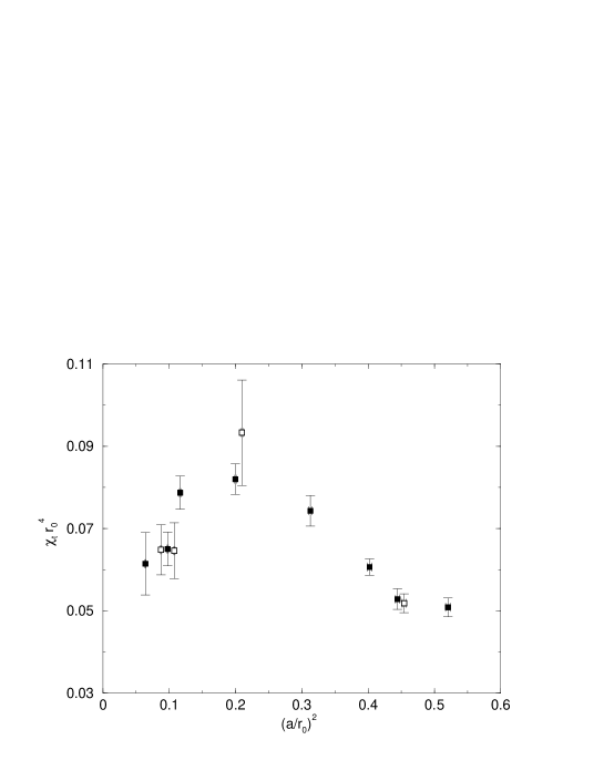
Figure 6.1: The quenched topological susceptibility $\chi_{t}$ measured with the overlap construction with $\operatorname{{\cal D}_{\rm par}}$. The open squares are used to denote in a clearer way that the corresponding symbol is shifted horizontally in order to display measurements done at the same scale, but with either different accuracy of the overlap construction or on different volumes. The decrease of $\chi_{t}$ towards coarse lattices (large $a$) is an artifact due to the fact that instantons fall through the lattice, i.e. they can no longer be resolved. The decrease towards small lattice spacings is much more important as it indicates clearly a cut-off effect.

6.1.3 Discussion

The results shown in Figure 6.2 give clearly the impression that the topological susceptibility measured with the overlap construction with $\operatorname{{\cal D}_{\rm par}}$ has substantial cut-off effects. But one has to keep several things in mind. The decrease towards coarse lattice spacings is expected as the lattice gets too coarse to resolve topological objects, i.e. instantons fall through the lattice, and the results for the very coarse lattice spacings are only given for completeness. Obviously more important is the decrease towards small lattice spacings, which really indicates a relevant cut-off effect. It can be understood in different ways. The measurement at the smallest lattice spacing, which with $a=0.13\,{\rm fm}$ is still not very fine, is not very accurate and the picture might change with more statistics. Furthermore, the determination of the scale enters with $(r_{0}/a)^{4}$ which makes that systematic errors become quite relevant. Clearly, the finite volume effects are not under control in this compilation of data and we can not exclude that the points at $\beta=3.2$ and $\beta=3.0$ are affected more by finite volume effects than the points at $\beta=2.927$ and $\beta=2.68$, which are measured on a larger volume. However, the finite volume effects are not expected to be large when the size of the box is $1.2\,{\rm fm}$ or more. Finally, we give a comparison to other recent measurements [149, 150] of the topological susceptibility. Our results do not show any obvious discrepancy with the other data as the lattice spacing gets small, however, neither our data nor the data of the other groups are as accurate that a more precise statement can be made at this point.

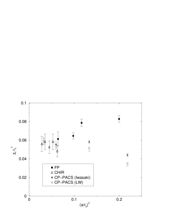
Figure 6.2: The quenched topological susceptibility obtained from different recent determinations. In this figure only the physically interesting part towards smaller lattice spacings is shown. We compare our results (FP), where we have combined the data from different determinations at the same lattice spacing in this figure, to the very recent determination in [150], which uses a truncated solution of the GW relation and counts the chirality of the small real modes (CHIR). The other two measurements are done by the CP-PACS collaboration and use traditional cooling techniques with the Iwasaki and the Lüscher-Weisz action [149].

6.2 Local Chirality of Near-Zero Modes

Exact zero modes of the Dirac operator tell us, via the index theorem, about the topological charge $Q$ of the background gauge configuration. However, the exact zero modes alone cannot break chiral symmetry spontaneously. According to the Banks-Casher relation [141] $\langle\bar{\psi}\psi\rangle=-\pi\rho(0)\neq 0$, the Dirac operator must build up a finite density of near-zero modes, which does not vanish as $V\rightarrow\infty$.

One mechanism which explains the formation of near-zero modes involves instantons. Consider a gauge configuration containing one instanton and one anti-instanton. If the instanton and anti-instanton are separated by a large distance, the Dirac operator has a pair of complex eigenvalues lying close to 0. The farther the instanton and anti-instanton are separated from each other, the closer the complex eigenvalue pair moves to the origin. If the instanton and anti-instanton are brought closer together, the complex eigenvalue pair moves away from the origin and disappears into the bulk of the eigenvalue spectrum. If the gauge configurations contain many instantons and anti-instantons, this could produce a non-zero density of near-zero modes, giving $\rho(0)\neq 0$ in the infinite volume limit.

The question has recently been raised if it is possible to show that the near-zero modes are dominated by instantons. From instanton physics, it is expected that the modes are highly localized where the instantons and anti-instantons sit. If this is so, then in these regions the modes should be close to chiral i.e. mostly either left- or right-handed, depending on whether it is sitting on an instanton or anti-instanton. In [151], the authors defined a measure of local chirality at lattice site $x$ by

$$\tan\left[\frac{\pi}{4}(1+X(x))\right]=\sqrt{\frac{{\psi_{\rm L}}^{\dagger}\psi_{\rm L}(x)}{{\psi_{\rm R}}^{\dagger}\psi_{\rm R}(x)}}.$$ (6.3)

An exact zero mode is purely either left- or right-handed, giving $X(x)=\pm 1$ at all lattice sites $x$. If a near-zero mode is localized around instanton-anti-instanton lumps, then $X(x)$ should be close to $\pm 1$ for the sites $x$ where the probability density $\psi^{\dagger}\psi(x)$ is largest.

In the original paper [151], many near-zero modes of the Wilson operator $D_{W}$ were analyzed for many gauge configurations and the finding was that in the regions where the modes are localized, the distribution for $X(x)$ is peaked around 0 and the modes do not display local chirality. This led to the conclusion that the near-zero modes are not dominated by instantons. Since then, several other groups have found the opposite conclusion [152, 117, 153, 154], using Dirac operators with much better chiral symmetry than $D_{W}$ (or even just an alternative definition of a complete basis for the non-normal operator $D_{W}$). They find the distribution of $X(x)$ is double-peaked with maxima at large positive and negative values of $X$, indicating that the modes are locally chiral.

6.2.1 Results

In our study we analyze the 10 smallest near-zero modes of the overlap operator with $\operatorname{\textfrak{D}_{\rm par}}$ as kernel for 60 different $10^{4}$ gauge configurations at $\beta=3.2$. We use a Legendre polynomial of order 2 to approximate the operator $(A^{\dagger}A)^{-1/2}$ in overlap formula, with the 10 smallest $A^{\dagger}A$ being projected out and treated exactly (see Chapter 5 for details). The eigenvalues $\lambda$ and eigenvectors $\psi$ are found using the implicitly restarted Arnoldi method [113, 114]. In Figure 6.3, we plot the distribution $P(X)$ of the measure of local chirality $X$ at the lattice sites where the density $\psi^{\dagger}\psi(x)$ of a mode is largest. The three distributions correspond to taking, for each mode, 1%, 5% and 10% of all lattice sites that have the largest density $\psi^{\dagger}\psi(x)$. We do not include exact zero modes, for which $X(x)=\pm 1$ at all lattice sites. We see a clear double-peaked distribution, whose maxima are farther from zero if we only include the sites where the modes are most localized. The maxima are not at $X=\pm 1$ as the modes are not exactly chiral. We find the same conclusion as [152, 117, 153, 154]: where the near-zero modes are most localized, they are also very chiral. Recent work [155] has shown that, using near-zero modes of the Dirac operator, the gauge field strength appears to contain lumps which are mostly either self-dual or anti-self-dual. This behavior is consistent with the picture of instanton-dominance of the near-zero modes, however it is no conclusive evidence that instantons are the driving mechanism for chiral symmetry breaking [156, 157].

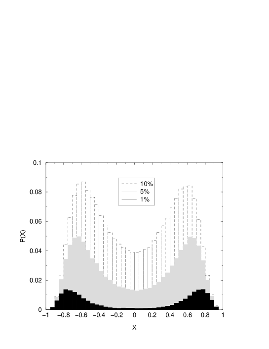
Figure 6.3: The distribution $P(X)$ for the top 1%,5%,10% lattice sites $x$ with the largest $\psi^{\dagger}\psi(x)$.

Chapter 7 Determination of the Low-Energy Constant $\Sigma$

It is the common expectation that for QCD with a number $N_{f}\geq 2$ of massless quark flavors, the chiral symmetry is spontaneously broken by a non-zero expectation value for the chiral condensate $\langle\bar{\psi}\psi\rangle$. Chiral perturbation theory ($\chi{\rm PT}$), which is based on this assumption, is an excellent description of many low-energy QCD phenomena [4]. However, it is only possible via lattice QCD to test from first principles if the symmetry is spontaneously broken.

The leading order effective theory of $\chi{\rm PT}$ contains the low-energy constants $f_{\pi}$ and $\Sigma$. In full QCD the Gell-Mann-Oakes-Renner relation (GMOR)

$$f_{\pi}^{2}m_{\pi}^{2}=4m\Sigma,$$ (7.1)

becomes exact in the $m\rightarrow 0$ chiral limit and the chiral condensate $\langle\bar{\psi}\psi\rangle=\langle\bar{u}u\rangle=\langle\bar{d}d\rangle=\dots$, defined at zero quark mass, is equal to -$\Sigma$. The low energy constant $\Sigma$ depends on the number of massless flavors $N_{f}$.

In quenched QCD, the relation $\langle\bar{\psi}\psi\rangle=-\Sigma$ and eq. (7.1) receive corrections even in the chiral limit [158, 159, 160]. Actually, $\langle\bar{\psi}\psi\rangle$ and $m_{\pi}^{2}/m$ are not even defined in the chiral limit due to diverging quenched chiral logarithms. In the case of $m_{\pi}^{2}/m$ the logarithms, which are characterized by the parameter $\delta$, are connected to the mass of the flavor singlet particle $\eta^{\prime}$, which is an additional Goldstone boson in Q$\chi{\rm PT}$ [159, 158]. The mass of the $\eta^{\prime}$ is an additional, third leading order low-energy constant $m_{0}$ of Q$\chi{\rm PT}$, which is not present in the normal $\chi{\rm PT}$ Lagrangian. The expectation that $m_{\pi}^{2}/m$ diverges in Q$\chi{\rm PT}$ in the chiral limit is confirmed by different measurements [161, 162, 163], including our hadron spectroscopy measurements with $\operatorname{\textfrak{D}_{\rm par}}$ [65]. Similarly, the divergence of $\langle\bar{\psi}\psi\rangle$ in the infinite volume limit seems to be confirmed in numerical studies of the Banks-Casher relation [164]. On the other hand, it is possible to study and determine the low-energy constant $\Sigma$ in the quenched theory. Under the assumption that $\Sigma(N_{f})$ is a smooth function of $N_{f}$ and $\Sigma(N_{f}=0)$ is close to $\Sigma(N_{f}=3)$ (which is the standard assumption when quenched results are used to estimate full QCD quantities) we get an estimate for the chiral condensate $-\langle\bar{\psi}\psi\rangle(N_{f}=3)=\Sigma(N_{f}=3)\approx\Sigma(N_{f}=0)$, even though it is hard to give a systematic error for this estimate. Typically, the quenching error are said to be of order $10-20\%$ [79].

On the lattice the calculation of the low-energy constant $\Sigma$ of (quenched) chiral perturbation theory requires good control over the chiral properties of the theory and therefore it has notoriously been difficult to measure it directly. Still, early attempts with staggered fermions have been tried already in 1985 [165] and the calculation can also be performed with other traditional discretizations, like ${\cal O}(a)$ improved Wilson fermions using Ward identities and the GMOR relation eq. (7.1) [166, 167]. However, the calculation is more transparent and cleaner in the framework of GW fermions due to many reasons. With Wilson fermions one has to deal with a power divergent subtraction that has to be determined numerically [166]. Furthermore, the occurrence of exceptional configurations makes it difficult to go to quark masses which are small enough to provide an accurate estimate for $\Sigma$ in the chiral limit. In the case of GW fermions chiral symmetry is already realized on the lattice [21]. This makes it possible to define scalar and pseudoscalar densities which transform under chiral transformations exactly like the corresponding continuum densities [52]. Using such a scalar density the power divergent subtraction, which has to be performed on the bare condensate, is exactly known and can be done without problems in numerical simulations [39]. A further advantage of GW fermions is that one does not encounter any exceptional configurations in the small quark mass regime. These facts altogether allow a much better control over the calculations.

There are different techniques to calculate $\Sigma$ with GW fermions. One possibility makes use of the GMOR relation and data from pseudoscalar spectroscopy [168]. Another possibility is to use the distribution of the lowest-lying eigenmodes of the massless Dirac operator, because these distribution can be described in the framework of random matrix theory (RMT) [169] and provide a completely different way to extract $\Sigma$. Actually, the distributions of the low-lying eigenmodes contain a lot more of information than the value of $\Sigma$ as explained in [170], but in leading order they are essentially described by $\Sigma$. A technique which is closely related to the determination of $\Sigma$ from the eigenvalue distributions is the so called finite-volume scaling technique, which has been worked out in [160], and has been used for the first time in [130]. In our calculation of $\Sigma$ we use a slightly modified version of this technique.

All the 3 different methods provide a bare value of $\Sigma$ that subsequently has to be renormalized in order to give the phenomenologically relevant predictions $\hat{\Sigma}$ and $\Sigma_{\overline{\rm MS}}(2{\rm GeV})$, respectively. Again, there are different possibilities how the scalar renormalization factor $Z_{S}$ can be calculated. It is known that lattice perturbation theory converges only slowly in many cases and is therefore very difficult to control in the range of gauge couplings where typical simulations are performed [171]. The way to circumvent this problem is the use a non-perturbative renormalization scheme. There are essentially two different non-perturbative renormalization schemes used in the present day lattice simulations. One scheme is the RI/MOM technique [172], which uses the fact that QCD can be treated perturbatively at large momentum scales, in order to match amputated quark Green functions to a perturbative scheme (e.g. $\overline{\rm MS}$), while the other scheme, the Schrödinger functional technique, is based on the fact that QCD in a very small volume can be treated perturbatively [171]. The size $L$ of the box acts as a reference scale and can e.g. be connected to the normalization mass in the $\overline{\rm MS}$ scheme using perturbative renormalization group arguments. We will follow the renormalization scheme proposed in [173], which is based – even though not directly – on the Schrödinger functional technique.

But, before we start to explain our determination of $\Sigma$, let us mention that more details of the calculation, in particular about the stochastic evaluation of the trace of the subtracted quark propagator, are given in Appendix E.

7.1 Determination of the Bare $\Sigma$

One possibility to determine $\Sigma$ is to study the chiral condensate in a fixed topological sector with charge $Q$ in a finite volume $V$ at finite quark mass $M$ [160]. The volume and the quark mass are chosen such that the finite size effects are dominated by the pions with zero momentum. In this situation the partition function simplifies considerably and can even be evaluated analytically in certain cases [174, 160]. Using (Q)$\chi{\rm PT}$, or random matrix theory (RMT), the fermion condensate at finite volume and quark mass has been calculated in the continuum, both for full and quenched QCD. The quenched QCD condensate $\langle\bar{\psi}\psi\rangle_{M,V,Q}$ can be written in terms of the derivative of the logarithm of the partition function ${\cal Z}_{Q}$ in fixed topology

$$-\langle\bar{\psi}\psi\rangle_{M,V,Q}=\frac{\partial}{\partial M}\ln{\cal Z_{Q}}\,,$$ (7.2)

with

$${\cal Z}_{Q}=\int_{{\rm Gl}(1|1)}dU_{0}{\rm Sdet}(U_{0}^{Q})\exp[V\Sigma{\rm Re\,Str[MU_{0}]}]\,,$$ (7.3)

where ${\rm Sdet}$ and ${\rm Str}$ are the supersymmetric generalizations of the determinant and the trace, respectively. The integration is over the graded Lie group ${\rm Gl}(1|1)$. For details of the supersymmetric formulation of Q$\chi{\rm PT}$ see [175, 159, 158, 160, 176, 170]. The analytic expression for this partition function is known [160] and therefore the condensate in fixed topology at mass $M$ is given by

$$-\langle\bar{\psi}\psi\rangle_{M,V,Q}=MV\Sigma^{2}[I_{|Q|}(z)K_{|Q|}(z)+I_{|Q|+1}(z)K_{|Q|-1}(z)]+\frac{|Q|}{MV},$$ (7.4)

where $I_{Q}$ and $K_{Q}$ are modified Bessel functions, $z=M\Sigma V$ and the low-energy constant $\Sigma$ is the quantity we wish to measure. By measuring $\langle\bar{\psi}\psi\rangle_{M,V,Q}$ in different topological sectors, at different masses and volumes, the continuum prediction of the $M$ and $V$ dependence can be used to extract $\Sigma$.

On the lattice the subtracted condensate in a fixed topological sector in a volume $V$ and with bare mass $m$ can be calculated by measuring the trace [39, 130]

$$-\langle\bar{\psi}\psi\rangle^{\rm sub}_{m,V,Q}=\frac{1}{V}\Big{\langle}{\rm Tr}^{\prime}\Big{[}\operatorname{\textfrak{D}}^{-1}(m)-R\Big{]}\Big{\rangle}_{Q}$$ (7.5)

with

$$\operatorname{\textfrak{D}}(m)=\Big{(}1-\frac{m}{2}\Big{)}\operatorname{\textfrak{D}}(0)+m(2R)^{-1}$$ (7.6)

and where the primed trace is without the divergent contribution of the zero modes and $\langle.\rangle_{Q}$ is the expectation value on the ensemble of gauge fields with topological charge $Q$. Because we want to make use of the renormalization scheme proposed by Hernández et al. in [173], which is based on pseudoscalar spectroscopy, we have to modify the strategy of the measurements performed in [130, 116] slightly. The reason for this is that in our hadron spectroscopy study [65] a mass definition $m$ is used which differs from the usual definition $M$ by a factor $2R$ (see e.g. eq. (7.6)). Instead of the trace in eq. (7.5), we use

$$-\langle S\rangle_{m,V,Q}=\frac{\partial}{\partial m}\ln{\cal Z_{Q}}=\frac{1}{V}\bigg{\langle}{\rm Tr}^{\prime}\bigg{[}(\operatorname{\textfrak{D}}(m)2R)^{-1}-\frac{1}{2}\operatorname{\textfrak{D}}(0)\operatorname{\textfrak{D}}^{-1}(m)\bigg{]}\bigg{\rangle}_{Q}\,.$$ (7.7)

The scalar density $S$ is the same as introduced in Chapter 5 and its properties are discussed in more details in [140], i.e.

$$S=\bar{\psi}\Big{(}(2R)^{-1}-\frac{1}{2}\operatorname{\textfrak{D}}(0)\Big{)}\psi\,.$$ (7.8)

The partition function $${\cal Z_{Q}}$$ is given by

$${\cal Z_{Q}}=\int DU_{Q}D\bar{\psi}D\psi\exp[-(\bar{\psi}\operatorname{\textfrak{D}}(0)\psi+mS)-{\cal A}_{g}]\,,$$ (7.9)

with the gauge action ${\cal A}_{g}$. Furthermore, the path integral is restricted to gauge fields with topological charge $Q$. For masses $m$ smaller than the modulus of the smallest eigenvalue $\lambda_{\rm min}$ of the massless Dirac operator $\operatorname{{\cal D}}$(0), i.e $m^{2}<|\lambda_{\rm min}|^{2}$, the trace in eq. (7.7) reduces to

$$-\langle S\rangle_{m,V,Q}=\frac{1}{V}\bigg{\langle}{\rm Tr}^{\prime}\bigg{[}(\operatorname{\textfrak{D}}(m)2R)^{-1}-\frac{1}{2}\bigg{]}\bigg{\rangle}_{Q}$$ (7.10)

up to terms of ${\cal O}(m^{2})$, as one can show easily. Because the numerical results show to be less sensitive to a residual breaking of chiral symmetry with the definition from eq. (7.10) than with eq. (7.7), we use the definition from eq. (7.10) for our measurements, which clearly agrees with the definition in eq. (7.7) in the chiral limit. The correlation function $\langle S\rangle_{m,V,Q}$ differs from $\langle\bar{\psi}\psi\rangle^{\rm sub}_{M,V,Q}$ by a factor $(2R)^{-1}$. Together with the scalar renormalization factor $Z_{S}$, which for chiral actions is given by $Z_{S}=1/Z_{m}$, however, the additional factor drops out in the physical prediction, because the additional factors from the mass definition and $\langle S\rangle_{m,V,Q}$ cancel. Let us be a bit more specific about what is meant with this: In our case the eigenvalue spectrum of the operator $2R$ is roughly bounded by $2/\kappa$ and $4/\kappa$ with $\kappa=3.45$ for our parametrization and therefore its eigenvalues are close to 1 and no exceptionally small or large eigenvalues can occur, which in a simulation might spoil the fact that the two additional factors of $(2R)^{-1}$ and $2R$ in $\langle S\rangle_{m,V,Q}$ and $m$, respectively, cancel to a high degree.

7.1.1 Details of the Simulation

We measure the trace in eq. (7.10) stochastically using random $Z(2)$ vectors [177]. In order to measure the condensate at very small quark mass, the remnant explicit chiral symmetry breaking must be very small, so we use the overlap operator with the kernel $\operatorname{{\cal D}_{\rm par}}$, as discussed in Chapter 5. Due to the $|Q|$ chiral zero modes of the Dirac operator, the quenched condensate contains a term $|Q|/MV$ which diverges as the mass becomes small. The $|Q|$ zero modes have the same chirality and their contribution to the condensate is removed by measuring the trace ${\rm Tr}^{\prime}$ in the chiral sector opposite to the zero modes [178, 130], i.e. if the $|Q|$ modes have chirality $+$, the $Z(2)$ vectors used to measure the trace are chosen to have chirality $-$. To determine $\langle S\rangle_{m,V,Q}$, the stochastic trace is doubled to include both chiral sectors.

We measure the condensate in volumes $8^{4}$ and $10^{4}$ at $\beta=3.2$. We use 10 random $Z(2)$ vectors to measure the trace for each configuration and a BiCGstab multi-mass solver to invert the Dirac operator at all 12 masses in the range $ma=0.0001,\ldots,0.2048$ simultaneously. In the overlap operator, we approximate $(A^{\dagger}A)^{-1/2}$ with Legendre polynomials of order 7 and 10 for volumes $8^{4}$ and $10^{4}$, respectively. We project out the 10 smallest $A^{\dagger}A$ eigenvalues, which are treated exactly. This altogether gives sufficiently precise chiral symmetry: increasing the polynomial order further, the relative change in the estimate of $(\langle S\rangle_{m,V,Q}a^{3})/(ma)$ is $\leq{\cal O}(10^{-4})$. This fact is shown in Figure 7.1, where the relative difference between the (nearly) exact result with a Legendre expansion of order $12$ and lower order expansions with order $N$ at $ma=10^{-4}$ for the quantity

$$\Delta(N)=\frac{\langle\phi|(\operatorname{\textfrak{D}}^{(N)}(m)2R)^{-1}-\frac{1}{2}|\phi\rangle-\langle\phi|(\operatorname{\textfrak{D}}^{(12)}(m)2R)^{-1}-\frac{1}{2}|\phi\rangle}{\langle\phi|(\operatorname{\textfrak{D}}^{(12)}(m)2R)^{-1}-\frac{1}{2}|\phi\rangle}\,,$$ (7.11)

where $\phi$ is a $Z(2)$ random vector, is shown for several $8^{4}$ configurations. Our statistics are given in Table 7.1. In Figure 7.2, we show the distribution of the estimates of $(\langle S\rangle_{m,V,Q}a^{3})/(ma)$ obtained from the different $Z(2)$ random vectors in $|Q|=1$ topological sector on the $8^{4}$ and $10^{4}$ configurations, respectively. One observes that the distributions have quite a long tail towards large values, especially on the $10^{4}$ lattice.

$L$	order	$|Q|$	$N_{\rm conf}$
8	7	1	154
		2	41
10	10	1	53
		2	43

Table 7.1: Polynomial order of $(A^{\dagger}A)^{-1/2}$ approximation and statistics for the measurement of $\Sigma$.

7.1.2 Results

Let us first explain how the bare value of $\Sigma$ can be extracted from eq. (7.4) and the measurements of the trace in eq. (7.10). The bare quark condensate at finite quark mass contains a $\sim m/a^{2}$ cut-off effect. As the quark mass $m\rightarrow 0$, one can rewrite eq. (7.4) such that

$$-\frac{\langle\bar{\psi}\psi\rangle^{\rm sub}_{M,V,Q}}{M}=-\alpha^{2}\frac{\langle S\rangle_{m,V,Q}}{m}=\frac{\Sigma^{2}V}{2|Q|}+\frac{c_{1}}{a^{2}},$$ (7.12)

where $c_{1}$ is an unknown coefficient, which has to be fitted, and $\alpha$ denotes the ratio between the different mass definitions: $\alpha=m/M$. As the coefficient $c_{1}$ comes from ultraviolet fluctuations, it is natural to assume that it is independent of the topological charge $Q$. The contribution of the $|Q|$ zero modes is removed by taking the trace as described above, and there is no artifact $1/(ma^{3})$ in eq. (7.12) due to the fact that the condensate is defined as the expectation value of a scalar operator that transforms covariantly under chiral transformations and has no mixing with the unit operator [39]. From Figure 7.3, we see that $-(\langle S\rangle_{m,V,Q}a^{3})/(ma)$ reaches a plateau at very small quark mass. In Figure 7.4, we plot the value of $-(\langle S\rangle_{m,V,Q}a^{3})/(ma)$ at $ma=10^{-4}$ versus $(Va^{-4})/2|Q|$, which we fit to the form of eq. (7.12). From the slope, we extract the bare low-energy constant as $\Sigma a^{3}=4.42(36)\times 10^{-3}$ with $\chi^{2}/df=3.55$. We can convert this result using the Sommer parameter ($r_{0}/a=3.943(60)$ at $\beta=3.2$ from the interpolating formula in [95]), giving $\Sigma r_{0}^{3}=0.271(22)(12)$, where the first error is statistical and the second the uncertainty in the scale.

Figure 7.1: In this figure the dependence of the relative difference $\Delta(N)$, defined in eq. (7.11), between the (nearly) exact overlap and lower order Legendre approximations with order $N$ is shown for several different $8^{4}$ configurations at $\beta=3.2$.

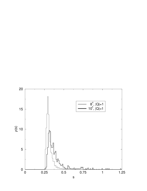
Figure 7.2: Normalized distribution $\rho(s)$ of the estimate of $s=(\langle S\rangle_{m,V,Q}a^{3})/(ma)$ at $ma=10^{-4}$ for the different $Z(2)$ random vectors and configurations used in the measurements is shown for the $Q=\pm 1$ sector on $8^{4}$ and $10^{4}$ configurations.

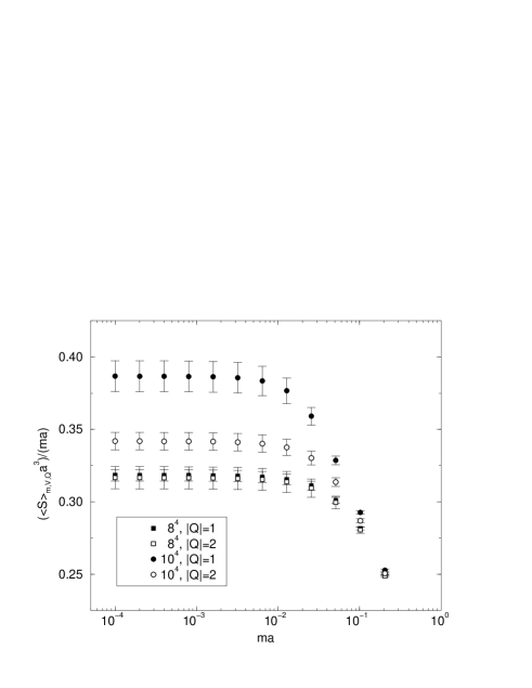
Figure 7.3: The estimated $(\langle S\rangle_{m,V,Q}a^{3})/(ma)$ for different volumes, masses and topological charges.

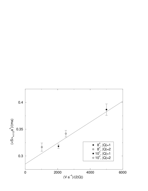
Figure 7.4: $(\langle S\rangle_{m,V,Q}a^{3})/(ma)$ for the smallest value of the mass $ma=10^{-4}$ plotted versus $(Va^{-4})/(2|Q|)$. The fit used to determine the slope is shown by the line.

7.2 Renormalization of $\Sigma$

In order to turn this bare result into the renormalized low-energy constant $\hat{\Sigma}$ we need the scalar renormalization factor $Z_{S}$. In the present test study we obtained $Z_{S}$ combining the continuum extrapolated renormalization group invariant (RGI) quark mass of the ALPHA collaboration [179] with our spectroscopy data. This method has been suggested recently by Hernández et al. [173]. Even though the method is based on the Schrödinger functional, the special boundary conditions of Schrödinger functional make a direct application to GW fermions difficult, if not impossible, and therefore improved Wilson fermions were used in an intermediate step. In the following we give a short description of the calculations done in [173] and apply the result to our data.

7.2.1 Short Introduction to the Technique

The idea of this technique is to connect the bare quark mass $m$ in the given discretization to the renormalization group invariant (RGI) quark mass $M$

$$M=Z_{M}(g_{0})m(g_{0})$$ (7.13)

and to use the fact that for lattice regularizations that preserve chiral symmetry the renormalization factor of the scalar density is the inverse of that for the quark mass (see, e.g. [180])

$$Z_{P}(g_{0})=Z_{S}(g_{0})=\frac{1}{Z_{M}(g_{0})}\,.$$ (7.14)

In order to fix $Z_{M}(g_{0})$ one can rewrite the ratio $M/m(g_{0})$ as

$$\frac{M}{m(g_{0})} =\frac{M}{m_{W}(g_{0}^{\prime})}\frac{m_{W}(g_{0}^{\prime})}{m(g_{0})}$$ (7.15)

$$=Z_{M}^{W}(g_{0}^{\prime})\frac{(r_{0}m_{W})(g_{0}^{\prime})}{(r_{0}m)(g_{0})}\,,$$ (7.16)

where $g_{0}^{\prime}\neq g_{0}$ in general, and the hadronic radius $r_{0}$ is used to set the scale. The factor $Z_{M}^{W}$ has been computed in [181] for a large range of couplings. The ratio $M/m(g_{0})$ is then obtained by determining $(r_{0}m)$ and $(r_{0}m_{W})$ at a reference value of $x_{\rm ref}$ of a physical observable, say $x_{\rm ref}=(r_{0}m_{P})^{2}$, where $m_{P}$ is the mass of the pseudoscalar meson. In order to get rid of discretization errors the combination $Z_{M}^{W}(g_{0}^{\prime})(r_{0}m_{W})(g_{0}^{\prime})$ was calculated in the continuum limit, i.e.

$$U_{M}=\lim_{g_{0}^{\prime}\to 0}Z_{M}^{W}(g_{0}^{\prime})(r_{0}m_{W})(g_{0}^{\prime})\,,$$ (7.17)

leading to the following results [173]

$$U_{M}=\begin{cases}0.181(6),&x_{\rm ref}=1.5736,\\ 0.349(9),&x_{\rm ref}=3.0,\\ 0.580(12),&x_{\rm ref}=5.0.\end{cases}$$ (7.18)

By combining (7.13), (7.15) and (7.17) one obtains

$$Z_{M}(g_{0})=U_{M}\frac{1}{(r_{0}m)}\Big{|}_{(r_{0}m_{P})^{2}=x_{\rm ref}}\,,$$ (7.19)

where now all reference to the bare coupling $g^{\prime}_{0}$ and the use of the intermediate Wilson fermions has disappeared. Apart from cut-off effects, $Z_{M}(g_{0})$ is expected to be independent of the reference point $x_{\rm ref}$.

7.2.2 Results

Using the results of the hadron spectroscopy with the overlap with $\operatorname{\textfrak{D}_{\rm par}}$ at $\beta=3.2$ [65], we are able to calculate the scalar renormalization factor $Z_{S}$. The pseudoscalar spectroscopy data is obtained from $32$ $9^{3}\times 24$ lattices. Because of the small statistics and the rather small volume the determination of the renormalization constants at $\beta=3.2$ has a rather large error. For our determination we combine data from the pseudoscalar - scalar (PS) and the axial-vector (A) correlator measurements of the pseudoscalar mass. The reason for this is that the PS correlator gets contributions from the scalar at high bare quark masses, while the A correlator is sensitive to the topological finite size effects caused by the zero modes at small bare quark masses [182]. Using this combined data, we fit a second order polynomial through the data points in the region $m=0.01,\ldots,0.17$ as shown in Figure 7.5.

Figure 7.5: The $(m_{P}a)^{2}$ versus $ma$ data used to determine the scalar renormalization factor at $\beta=3.2$. The solid line is a fit using a second order polynomial, while the dot-dashed lines indicate the three reference values for the pseudoscalar mass $x_{\rm ref}=(r_{0}m_{P})^{2}=1.5736,3.0,5.0$ used to extract $Z_{M}$.

With these fits we determine the bare quark at which the pseudoscalar takes on the three reference values $x_{\rm ref}=(r_{0}m_{P})^{2}=1.5736,3.0,5.0$. We obtain

$$(r_{0}m)|_{(r_{0}m_{P})^{2}=x_{\rm ref}}=\begin{cases}0.141(24),&x_{\rm ref}=1.5736,\\ 0.271(36),&x_{\rm ref}=3.0,\\ 0.447(24),&x_{\rm ref}=5.0,\end{cases}$$ (7.20)

where we use the hadronic scale $r_{0}/a=3.943(60)$ from the interpolating formula in [95] to set the scale. In the determination of the $r_{0}m$ values a small additive mass renormalization $a\Delta_{m}=0.005(4)$ is taken into account. This residual additive mass renormalization is due to the fact that in the determination of the pseudoscalar spectrum a Legendre expansion of order 3 was used. This leaves place for a breaking of the GW relation which is large enough to give rise to a residual mass on the order of $10^{-3}$.

Using (7.19), we can combine the results for the bare quark masses in (7.20) with the universal factor $U_{M}$ from (7.18) and obtain the mass and scalar renormalization factors. The results are given in the Table 7.2.

$x_{\rm ref}$	$Z_{M}(g_{0})$	$Z_{S}(g_{0})$
1.5736	1.28(25)	0.78(15)
3.0	1.29(12)	0.78(7)
5.0	1.30(7)	0.77(4)

Table 7.2: Renormalization factors at $\beta$=3.2 for the different reference values of the pseudoscalar mass.

The dependence on the value of $x_{\rm ref}$ is weak and well covered by the statistical uncertainty. Following the arguments in [173] we choose the value at $x_{\rm ref}=3.0$ as our best estimate of the renormalization constant, and thus we obtain the following final result for the renormalization factor $Z_{M}(g_{0})=1.29(12)$ and $Z_{S}(g_{0})=0.869(32)$, respectively. These renormalization factors can be converted into the $\overline{\rm MS}$ scheme at the reference scale $\mu=2$ GeV using the results from [179]

$$\frac{\overline{m}_{\overline{\rm MS}}(\mu)}{M}=\frac{Z_{m}(g_{0},\mu)}{Z_{M}(g_{0})}=0.72076,\qquad\mu=2\,\text{GeV}\,,$$ (7.21)

with an error of $1.5\%$ due to the uncertainty in the quenched value of $\Lambda_{\overline{\rm MS}}$. This leads to $Z_{M}(g_{0},\mu)=0.93(9)$ and $Z_{S}(g_{0},\mu)=1.08(10)$, respectively.

We can combine the scalar renormalization factor with the bare value of $\Sigma$, which leads to the final prediction for the physical value of $\hat{\Sigma}$ and $\Sigma_{\overline{\rm MS}}(2{\rm GeV})$. We get

$$r_{0}^{3}\hat{\Sigma} =0.210(17)(9)(20)\,,$$ (7.22)

$$r_{0}^{3}\Sigma_{\overline{\rm MS}}(2{\rm GeV}) =0.291(24)(12)(28)\,,$$ (7.23)

with statistical, scale and renormalization errors, respectively. Combining all errors, but the error associated with the scale ambiguity in quenched QCD in quadrature and using $r_{0}=0.5\,{\rm fm}$, we find at $\beta=3.2$

$$\hat{\Sigma} =(235\pm 11\,{\rm MeV})^{3}\times\bigg{(}\frac{a^{-1}[{\rm MeV}]}{1556\,{\rm MeV}}\bigg{)}^{3}\,,$$ (7.24)

$$\Sigma_{\overline{\rm MS}}(2{\rm GeV}) =(262\pm 12\,{\rm MeV})^{3}\times\bigg{(}\frac{a^{-1}[{\rm MeV}]}{1556\,{\rm MeV}}\bigg{)}^{3}\,.$$ (7.25)

These results are still subject to discretization errors and clearly it would be desirable to have data at smaller lattice spacings in order to make a continuum extrapolation.

Using the GMOR relation from eq. (7.1), our result for $\Sigma$ and the slope $B$ in the $m_{\pi}^{2}$ vs. $m$ plot, which we determine to $aB=2.90(12)$, we can make a consistency check of our measurements. We get $af_{\pi}=78(4)\times 10^{-3}$, which corresponds to

$$f_{\pi}=(121.5\pm 5.9\,{\rm MeV})\times\bigg{(}\frac{a^{-1}[{\rm MeV}]}{1556\,{\rm MeV}}\bigg{)}\,,$$ (7.26)

i.e. we get sufficiently close to the value from other determinations of $f_{\pi}$ in quenched QCD, e.g. [183], which are quite close to the experimental value $f_{\pi}=131\,{\rm MeV}$, to be confident that no big systematic errors are induced through the low statistics or the small volumes we used in this study.

7.3 Discussion

The result of this determination of the low-energy constant $\Sigma$ in quenched QCD is in very good agreement with other recent determinations with chiral fermions [173, 115, 168], as shown in Figure 7.6. One should, however, mention that these studies – including ours – are based on poor statistics and the simulations were done in small physical volumes, which means that all these studies have a certain test character. Furthermore, none of these studies contains a continuum extrapolation. The small volume is a problem because the RMT prediction of the distribution of the low-lying eigenmodes is only valid up to the Thouless energy [184, 185], which means that only a small fraction of the eigenmodes are described properly. This clearly leads to a systematic error. The problem of small statistics is enhanced through the fact the trace in eq. (7.10) gets large contributions from the smallest eigenvalues of the Dirac operator. Hence, it is probable that the results are distorted by the very rare but sizeable contributions from very small eigenmodes and therefore we think that the statement in [185] that the distributions of the lowest-lying eigenvalues of the Dirac operator would provide an approach to the determination of $\Sigma$, which has smaller systematic errors, is most likely true.

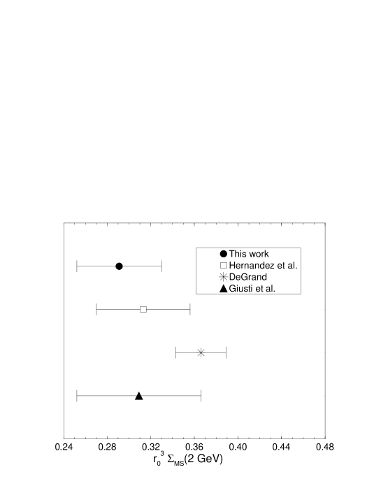
Figure 7.6: Comparison of different recent determinations of $r_{0}^{3}\Sigma_{\overline{\rm MS}}(2{\rm GeV})$.

Chapter 8 Conclusions and Prospects

The parametrized FP Dirac operator

In this work we have presented the construction and parametrization of a FP Dirac operator using a general hypercubic ansatz for the parametrization. We have shown how general Dirac operators can be constructed in an efficient way such that it is feasible to use them in numerical simulations. We have discussed the details of the parametrization procedure and have shown where the main difficulties lie. The properties of the resulting parametrization of the FP Dirac operator $\operatorname{\textfrak{D}_{\rm par}}$ have been investigated. We have found that the parametrization has clearly improved chiral behaviour with respect to the most frequently used lattice Dirac operator, the Wilson Dirac operator $D_{W}$. This fact is most evidently seen in the eigenvalue distribution of the operator $A^{\dagger}A$, which for a Dirac operator satisfying the Ginsparg-Wilson relation is equal to $1$. It deviates much less from $1$ for $\operatorname{\textfrak{D}_{\rm par}}$ than for $D_{W}$. Furthermore, we have found that the Krylow space methods used to calculate the eigenvalues and eigenvectors of the operator $A^{\dagger}A$, which are important for an efficient numerical implementation of the overlap construction, use substantially less operator times vector multiplications in the case of $\operatorname{\textfrak{D}_{\rm par}}$ than for $D_{W}$. We have found that the difference in the number of operator vector products can get so large that the determination of the low-lying eigenmodes of $A^{\dagger}A$ actually is only very little more expensive for $\operatorname{\textfrak{D}_{\rm par}}$ than for $D_{W}$, even though one matrix vector multiplication is ${\cal O}(40)$ times more expensive than for $D_{W}$. We have shown that the additive mass renormalization and the fluctuations of the low-lying eigenmodes of the Dirac operator are small, such that hadron spectroscopy simulations at remarkably small quark masses can be performed. Because of the possibility to go to very small quark masses clear signs of quenched chiral logarithms have been found in our hadron spectroscopy, which is described in detail in the thesis of Simon Hauswirth [65]. In the same study we have found that the scaling properties of $\operatorname{\textfrak{D}_{\rm par}}$ are, indeed, clearly improved to $D_{W}$ and ${\cal O}(a)$ scaling violations can not not be seen, even though more precise studies are needed to give a more quantitative statement. Finally, we have found that the definition of the topological charge through $\operatorname{Tr}(\gamma_{5}R_{\rm par}\operatorname{\textfrak{D}_{\rm par}})$ is problematic with the present parametrization as it deviates substantially from the index of $\operatorname{\textfrak{D}_{\rm par}}$, i.e. it does not satisfy the index theorem.

Overlap construction with $\operatorname{\textfrak{D}_{\rm par}}$

We have shown that the overlap construction with $\operatorname{\textfrak{D}_{\rm par}}$ is clearly more local in the sense that its couplings fall off faster than the common construction with $D_{W}$. In contrast to the Wilson overlap there is no need to fine tune a mass parameter to get optimal convergence or optimal locality in the overlap expansion with $\operatorname{\textfrak{D}_{\rm par}}$. We have found that polynomial approximations to the overlap construction with $\operatorname{\textfrak{D}_{\rm par}}$ converge very fast, i.e. that chiral symmetry up to machine precision can be reached with Legendre polynomial expansions of ${\cal O}(20)$ for the lattice sizes and gauge couplings used in this work. It has shown that such a precision, however, is barely needed in most simulations. We have found that low order expansions can be used in many cases to get enough accuracy for the chiral properties of the Dirac operator.

Physical Results

We have used low order polynomial approximations to the overlap construction with $\operatorname{\textfrak{D}_{\rm par}}$ to calculate the quenched topological susceptibility at various lattice spacings and volumes. The results point in the same direction as other recent results. However, our data is not yet accurate enough to allow for a controlled continuum extrapolation and shows cut-off effects. We also confirm the findings of various other groups about the local chirality of the near-zero modes of a Dirac operator, which might result from instanton dominance in the QCD vacuum. Finally, we have determined the low-energy constant $\Sigma$ of quenched chiral perturbation theory using a finite-volume scaling technique in a test study. Our result for the renormalized $\Sigma$ is

$$r_{0}^{3}\Sigma_{\overline{\rm MS}}(2\,{\rm GeV})=0.291(24)(12)(28)\,\,\,\text{at}\,\,\beta=3.2\,,$$

with statistical, scale and renormalization errors, respectively. This result does not include a continuum extrapolation and therefore is still subject to discretization errors. Converting to physical units by using the scale $r_{0}=0.5\,{\rm fm}$, which is somewhat problematic due to the scale ambiguity in quenched QCD, we get

$$\Sigma_{\overline{\rm MS}}(2\,{\rm GeV})=(262\pm 12\,{\rm MeV})^{3}\times\bigg{(}\frac{a^{-1}[{\rm MeV}]}{1556\,{\rm MeV}}\bigg{)}^{3}\,\,\,\text{at}\,\,\beta=3.2\,,$$

where all errors are combined in quadrature. This result is in good agreement with other recent studies of $\Sigma$ using chiral fermions. It should be mentioned that all these studies, including ours, are based on rather small statistics. Nevertheless, we have shown that with $\operatorname{\textfrak{D}_{\rm par}}$ we can use low order polynomial approximations to the overlap construction to perform calculations where chiral symmetry is needed to high precision.

Prospects

Let us start with the most obvious weakness of the present parametrization: The topological charge definition through $\operatorname{Tr}(\gamma_{5}R_{\rm par}\operatorname{\textfrak{D}_{\rm par}})$. In the present parametrization no special attention has been given to the pseudoscalar part of the parametrization and it is presently under study whether this weakness can be fixed with additional care in the parametrization process. If this is possible it would provide a numerically very cheap definition of the topological charge and moreover of the topological charge density. The overlap construction with $\operatorname{\textfrak{D}_{\rm par}}$ is suited to study the structure of topological excitations of the QCD vacuum, because there are indications that this overlap construction can resolve the underlying structure of the gauge fields better than the Wilson overlap. Using approximations to the overlap operator with $\operatorname{\textfrak{D}_{\rm par}}$, or simply $\operatorname{\textfrak{D}_{\rm par}}$ itself, further problems where chiral symmetry plays an essential rôle might be investigated, because the list of such problems is long. Let us mention just a few: Determination of further low-energy constants of (quenched) chiral perturbation theory, determination of quark masses of the light quarks, the resolution of the Kaplan-Manohar ambiguity in the first non-leading order Lagrangian of chiral perturbation theory and the calculation of the pion scattering length. Using the available data from the present study on hadron spectroscopy some of these problems can already be tackled. The data contains information about the pion decay constant, the light quark masses and further information about the parameter $\delta$ describing the quenched chiral logarithms. In order to extract some of this data one might use e.g. the RI/MOM scheme to calculate renormalization factors accurately. In connection with this renormalization scheme, which is sensitive to momentum cut-off effects, the good energy-momentum dispersion relation of $\operatorname{\textfrak{D}_{\rm par}}$ might be a big virtue. Furthermore, first applications of conserved chiral currents, which we proposed in [69, 140], might be interesting and useful.

Appendix A Representation of the Clifford Algebra

In this appendix we give the explicit representation of the $16$ elements of the basis of the Clifford algebra in the Weyl representation, as they are used throughout this work. In the current implementation of the programs for the parametrized FP Dirac operator the same convetions are used.

Scalar

$$\Gamma_{1}=1=\begin{pmatrix}1&0&0&0\\ 0&1&0&0\\ 0&0&1&0\\ 0&0&0&1\\ \end{pmatrix}$$ (A.1)

Vector

$$\Gamma_{2} =\gamma_{1}=\begin{pmatrix}0&0&0&-\rm i\\ 0&0&-\rm i&0\\ 0&\rm i&0&0\\ \rm i&0&0&0\\ \end{pmatrix} \Gamma_{3} =\gamma_{2}=\begin{pmatrix}0&0&0&-1\\ 0&0&1&0\\ 0&1&0&0\\ -1&0&0&0\\ \end{pmatrix}$$

$$\Gamma_{4} =\gamma_{3}=\begin{pmatrix}0&0&-\rm i&0\\ 0&0&0&\rm i\\ \rm i&0&0&0\\ 0&-\rm i&0&0\\ \end{pmatrix} \Gamma_{5} =\gamma_{4}=\begin{pmatrix}0&0&1&0\\ 0&0&0&1\\ 1&0&0&0\\ 0&1&0&0\\ \end{pmatrix}$$ (A.2)

Tensor

$$\Gamma_{6} =\rm i\sigma_{12}=\begin{pmatrix}\rm i&0&0&0\\ 0&-\rm i&0&0\\ 0&0&\rm i&0\\ 0&0&0&-\rm i\\ \end{pmatrix} \Gamma_{7} =\rm i\sigma_{13}=\begin{pmatrix}0&-1&0&0\\ 1&0&0&0\\ 0&0&0&-1\\ 0&0&1&0\\ \end{pmatrix}$$

$$\Gamma_{8} =\rm i\sigma_{14}=\begin{pmatrix}0&-\rm i&0&0\\ -\rm i&0&0&0\\ 0&0&0&\rm i\\ 0&0&\rm i&0\\ \end{pmatrix} \Gamma_{9} =\rm i\sigma_{23}=\begin{pmatrix}0&\rm i&0&0\\ \rm i&0&0&0\\ 0&0&0&\rm i\\ 0&0&\rm i&0\\ \end{pmatrix}$$

$$\Gamma_{10} =\rm i\sigma_{24}=\begin{pmatrix}0&-1&0&0\\ 1&0&0&0\\ 0&0&0&1\\ 0&0&-1&0\\ \end{pmatrix} \Gamma_{11} =\rm i\sigma_{34}=\begin{pmatrix}-\rm i&0&0&0\\ 0&\rm i&0&0\\ 0&0&\rm i&0\\ 0&0&0&-\rm i\\ \end{pmatrix}$$ (A.3)

Pseudoscalar

$$\Gamma_{12}=\gamma_{5}=-\gamma_{1}\gamma_{2}\gamma_{3}\gamma_{4}=\begin{pmatrix}-1&0&0&0\\ 0&-1&0&0\\ 0&0&1&0\\ 0&0&0&1\\ \end{pmatrix}$$ (A.4)

Axial-vector

$$\Gamma_{13} =\gamma_{1}\gamma_{5}=\begin{pmatrix}0&0&0&-\rm i\\ 0&0&-\rm i&0\\ 0&-\rm i&0&0\\ -\rm i&0&0&0\\ \end{pmatrix} \Gamma_{14} =\gamma_{2}\gamma_{5}=\begin{pmatrix}0&0&0&-1\\ 0&0&1&0\\ 0&-1&0&0\\ 1&0&0&0\\ \end{pmatrix}$$

$$\Gamma_{15} =\gamma_{3}\gamma_{5}=\begin{pmatrix}0&0&-\rm i&0\\ 0&0&0&\rm i\\ -\rm i&0&0&0\\ 0&\rm i&0&0\\ \end{pmatrix} \Gamma_{16} =\gamma_{4}\gamma_{5}=\begin{pmatrix}0&0&1&0\\ 0&0&0&1\\ -1&0&0&0\\ 0&-1&0&0\\ \end{pmatrix}$$ (A.5)

Appendix B The List of Factorized Contributions

In this appendix we provide a factorization of the paths used in the program code of the parametrized FP Dirac operator. The correspondig reference paths and their properties are given in the Tables 2.1-2.5.

B.1 Definitions

We introduce the operator $\hat{U}_{\mu}$ of the parallel transport for direction $\mu$

$$\left(\hat{U}_{\mu}\right)_{nn^{\prime}}=U_{\mu}(n)\delta_{n+\hat{\mu},n^{\prime}}\,,$$ (B.1)

and analogously for the opposite direction

$$\left(\hat{U}_{-\mu}\right)_{nn^{\prime}}=U_{\mu}(n-\hat{\mu})^{\dagger}\delta_{n-\hat{\mu},n^{\prime}}\,.$$ (B.2)

It is also useful to introduce the operator $\hat{U}(l)$ of the parallel transport along some path $l=[l_{1},l_{2},\ldots,l_{k}]$ where $l_{i}=\pm 1,\ldots,\pm 4$, by

$$\hat{U}(l)=\hat{U}_{l_{1}}\hat{U}_{l_{2}}\ldots\hat{U}_{l_{k}}\,.$$ (B.3)

In terms of gauge links this is

$$\left(\hat{U}(l)\right)_{nn^{\prime}}=\left(U_{l_{1}}(n)U_{l_{2}}(n+\hat{l}_{1})\ldots\right)\delta_{n+r_{l},n^{\prime}}\,,$$ (B.4)

We define the plaquette products (i.e. the operators of parallel transport along a plaquette) in the following way:

$$P_{l_{1},l_{2}}=\hat{U}([l_{1},l_{2},-l_{1},-l_{2}])\,,$$ (B.5)

where $l_{i}=\pm 1,\ldots,\pm 4$. Their hermitian conjugate is given by $(P_{l_{1},l_{2}})^{\dagger}=P_{l_{2},l_{1}}$. Reflections and permutations act on them in an obvious way.

We also define the staple products as

$$S_{l_{1},l_{2}}=\hat{U}([l_{1},l_{2},-l_{1}])\,.$$ (B.6)

We have $(S_{l_{1},l_{2}})^{\dagger}=S_{l_{1},-l_{2}}$.

To describe the shortest path to an offset we introduce the notation

$$V_{l_{1}}=\hat{U}([l_{1}])\,,$$

$$V_{l_{1},l_{2}}=\hat{U}([l_{1},l_{2}])\,,$$

$$V_{l_{1},l_{2},l_{3}}=\hat{U}([l_{1},l_{2},l_{3}])\,,$$ (B.7)

$$V_{l_{1},l_{2},l_{3},l_{4}}=\hat{U}([l_{1},l_{2},l_{3},l_{4}])\,.$$

Introduce the following linear combinations transforming in a simple way under reflections:

$$P^{(++)}_{\mu\nu}=P_{\mu,\nu}+P_{\mu,-\nu}+P_{-\mu,\nu}+P_{-\mu,-\nu}\,,$$

$$P^{(+-)}_{\mu\nu}=P_{\mu,\nu}-P_{\mu,-\nu}+P_{-\mu,\nu}-P_{-\mu,-\nu}\,,$$ (B.8)

$$P^{(-+)}_{\mu\nu}=P_{\mu,\nu}+P_{\mu,-\nu}-P_{-\mu,\nu}-P_{-\mu,-\nu}\,,$$

$$P^{(--)}_{\mu\nu}=P_{\mu,\nu}-P_{\mu,-\nu}-P_{-\mu,\nu}+P_{-\mu,-\nu}\,.$$

The signs in the superscript denote the parity for reflections of the $\mu$, $\nu$ axes, respectively. Hermitian conjugation acts as interchanging both upper and lower indices, permutations simply by $\mu\to p_{\mu}$, $\nu\to p_{\nu}$.

It is also useful to denote combinations which are symmetric/antisymmetric with respect to interchanging the axes:

$$P^{\rm(sym)}_{\mu\nu}=P^{(++)}_{\mu,\nu}+P^{(++)}_{\nu,\mu}=P^{(++)}_{\mu,\nu}+{\rm h.c.}\,,$$ (B.9)

$$P^{\rm(as)}_{\mu\nu}=P^{(--)}_{\mu,\nu}-P^{(--)}_{\nu,\mu}=P^{(--)}_{\mu,\nu}-{\rm h.c.}\,.$$

For the staples we write

$$S^{(\nu,+)}_{\mu}=S_{\nu,\mu}+S_{-\nu,\mu}\,,$$

$$S^{(\nu,-)}_{\mu}=S_{\nu,\mu}-S_{-\nu,\mu}\,,$$ (B.10)

$$S^{(\nu,+)}_{-\mu}=S_{\nu,-\mu}+S_{-\nu,-\mu}\,,$$

$$S^{(\nu,-)}_{-\mu}=S_{\nu,-\mu}-S_{-\nu,-\mu}\,.$$

The subscript $\pm\mu$ denotes the direction of the staple, the superscript specifies the plane $\mu\nu$ and the parity in $\nu$.

For a line of length 2 we have

$$V^{(++)}_{\mu\nu}=V_{\mu,\nu}+V_{\mu,-\nu}+V_{-\mu,\nu}+V_{-\mu,-\nu}\,,$$

$$V^{(+-)}_{\mu\nu}=V_{\mu,\nu}-V_{\mu,-\nu}+V_{-\mu,\nu}-V_{-\mu,-\nu}\,,$$ (B.11)

$$V^{(-+)}_{\mu\nu}=V_{\mu,\nu}+V_{\mu,-\nu}-V_{-\mu,\nu}-V_{-\mu,-\nu}\,,$$

$$V^{(--)}_{\mu\nu}=V_{\mu,\nu}-V_{\mu,-\nu}-V_{-\mu,\nu}+V_{-\mu,-\nu}\,,$$

and analogously for longer lines. In analogy to eq. (B.9) we introduce the completely (anti)symmetric combinations $V^{\rm(sym)}_{\mu\nu\ldots}$, $V^{\rm(as)}_{\mu\nu\ldots}$ for the line products.

We also introduce the “4d plaquette”

$$Q_{l_{1},l_{2},l_{3},l_{4}}=\hat{U}([l_{1},l_{2},l_{3},l_{4},-l_{1},-l_{2},-l_{3},-l_{4}])\,,$$ (B.12)

and the odd combination $Q_{l_{1},l_{2},l_{3},l_{4}}^{(----)}$.

To simplify the expressions below, we require that all the directions entering $P_{l_{1},l_{2}}$, $S_{l_{1},l_{2}}$, $V_{l_{1},l_{2},\ldots}$, etc. are different, i.e. they are taken to be zero if e.g. $|l_{1}|=|l_{2}|$.

Below we list terms for the different choices of $\Gamma_{0}$ and $l_{0}$ used in current implementation of the parametrized FP Dirac operator code. The notation $\left.\sum\right.^{\prime}$ indicates that all indices in the corresponding sum are taken to be different.

B.2 The Offset $r_{0}=(0,0,0,0)$

$\Gamma_{0}=1$, $l_{0}=[\,]$

$$1\,.$$ (B.13)

$\Gamma_{0}=1$, $l_{0}=[1,2,-1,-2]$

$$\frac{1}{48}\sum_{\mu<\nu}P^{\rm(sym)}_{\mu\nu}\,.$$ (B.14)

$\Gamma_{0}=\gamma_{1}$, $l_{0}=[1,2,-1,-2]$

$$\frac{1}{24}\left.\sum_{\mu\nu}\right.^{\prime}\gamma_{\mu}\left(P^{(-+)}_{\mu\nu}-\mbox{h.c.}\right)\,.$$ (B.15)

$\Gamma_{0}=i\sigma_{12}$, $l_{0}=[1,2,-1,-2]$

$$\frac{1}{8}\sum_{\mu<\nu}i\sigma_{\mu\nu}P^{\rm(as)}_{\mu\nu}\,.$$ (B.16)

$\Gamma_{0}=\gamma_{5}$, $l_{0}=[1,2,-1,-2,3,4,-3,-4]$

$$\frac{1}{384}\gamma_{5}\left.\sum_{\mu\nu\rho\sigma}\right.^{\prime}\frac{1}{4}\epsilon_{\mu\nu\rho\sigma}P^{\rm(as)}_{\mu\nu}P^{\rm(as)}_{\rho\sigma}\,.$$ (B.17)

$\Gamma_{0}=\gamma_{5}$, $l_{0}=[1,2,3,4,-1,-2,-3,-4]$

$$\frac{1}{384}\gamma_{5}\left.\sum_{\mu\nu\rho\sigma}\right.^{\prime}\epsilon_{\mu\nu\rho\sigma}Q_{\mu\nu\rho\sigma}^{(----)}\,.$$ (B.18)

$\Gamma_{0}=\gamma_{1}\gamma_{5}$, $l_{0}=[1,2,-1,-2,3,4,-3,-4]$

$$\frac{1}{192}\left.\sum_{\mu\nu\rho\sigma}\right.^{\prime}\gamma_{\mu}\gamma_{5}\frac{1}{2}\epsilon_{\mu\nu\rho\sigma}\left(P^{(+-)}_{\mu\nu}P^{\rm(as)}_{\rho\sigma}+\mbox{h.c.}\right)\,.$$ (B.19)

$\Gamma_{0}=\gamma_{1}\gamma_{5}$, $l_{0}=[2,1,-2,-1,3,4,-3,-4]$

$$\frac{1}{192}\left.\sum_{\mu\nu\rho\sigma}\right.^{\prime}\gamma_{\mu}\gamma_{5}\frac{1}{2}\epsilon_{\mu\nu\rho\sigma}\left(P^{(-+)}_{\nu\mu}P^{\rm(as)}_{\rho\sigma}+\mbox{h.c.}\right)\,.$$ (B.20)

B.3 The Offset $r_{0}=(1,0,0,0)$

$\Gamma_{0}=1$, $l_{0}=[1]$

$$\sum_{\mu}\left(V_{\mu}+V_{-\mu}\right)\,.$$ (B.21)

$\Gamma_{0}=1$, $l_{0}=[2,1,-2]$

$$\frac{1}{6}\left.\sum_{\mu\nu}\right.^{\prime}\left(S^{(\nu,+)}_{\mu}+S^{(\nu,+)}_{-\mu}\right)\,.$$ (B.22)

$\Gamma_{0}=1$, $l_{0}=[2,3,1,-3,-2]$

$$\frac{1}{24}\left.\sum_{\mu\nu\rho}\right.^{\prime}\left(V_{\rho}S^{(\nu,+)}_{\mu}V_{-\rho}+V_{-\rho}S^{(\nu,+)}_{\mu}V_{\rho}+{\rm h.c.}\right)\,.$$ (B.23)

$\Gamma_{0}=\gamma_{1}$, $l_{0}=[1]$

$$\sum_{\mu}\gamma_{\mu}\left(V_{\mu}-V_{-\mu}\right)\,.$$ (B.24)

$\Gamma_{0}=\gamma_{1}$, $l_{0}=[2,1,-2]$

$$\frac{1}{6}\left.\sum_{\mu\nu}\right.^{\prime}\gamma_{\mu}\left(S^{(\nu,+)}_{\mu}-S^{(\nu,+)}_{-\mu}\right)\,.$$ (B.25)

$\Gamma_{0}=\gamma_{2}$, $l_{0}=[1,2,3,-2,-3]$

$$\frac{1}{16}\left.\sum_{\mu\nu\rho}\right.^{\prime}\,\gamma_{\nu}\left(V_{\mu}P^{(-+)}_{\nu\rho}-P^{(+-)}_{\rho\nu}V_{\mu}-{\rm h.c.}\right)\,.$$ (B.26)

$\Gamma_{0}=i\sigma_{12}$, $l_{0}=[2,1,-2]$

$$\frac{1}{2}\left.\sum_{\mu\nu}\right.^{\prime}i\sigma_{\mu\nu}\frac{1}{2}\left(S^{(\nu,-)}_{\mu}-S^{(\mu,-)}_{\nu}-\mbox{h.c.}\right)\,.$$ (B.27)

$\Gamma_{0}=i\sigma_{23}$, $l_{0}=[1,2,3,-2,-3]$

$$\frac{1}{16}\left.\sum_{\mu\nu\rho}\right.^{\prime}i\sigma_{\mu\nu}\frac{1}{2}\left(V_{\rho}P^{\rm(as)}_{\mu\nu}+P^{\rm(as)}_{\mu\nu}V_{\rho}-\mbox{h.c.}\right)\,.$$ (B.28)

$\Gamma_{0}=\gamma_{5}$, $l_{0}=[2,1,-2,3,4,-3,-4]$

$$\frac{1}{96}\gamma_{5}\left.\sum_{\mu\nu\rho\sigma}\right.^{\prime}\frac{1}{2}\epsilon_{\mu\nu\rho\sigma}\left(S^{(\nu,-)}_{\mu}P^{\rm(as)}_{\rho\sigma}+P^{\rm(as)}_{\rho\sigma}S^{(\nu,-)}_{\mu}+\mbox{h.c.}\right)\,.$$ (B.29)

$\Gamma_{0}=\gamma_{1}\gamma_{5}$, $l_{0}=[2,1,-2,3,4,-3,-4]$

$$\frac{1}{96}\left.\sum_{\mu\nu\rho\sigma}\right.^{\prime}\gamma_{\mu}\gamma_{5}\frac{1}{2}\epsilon_{\mu\nu\rho\sigma}\left(S^{(\nu,-)}_{\mu}P^{\rm(as)}_{\rho\sigma}-P^{\rm(as)}_{\rho\sigma}S^{(\nu,-)}_{\mu}+\mbox{h.c.}\right)\,.$$ (B.30)

$\Gamma_{0}=\gamma_{2}\gamma_{5}$, $l_{0}=[1,3,4,-3,-4]$

$$\frac{1}{16}\left.\sum_{\mu\nu\rho\sigma}\right.^{\prime}\gamma_{\nu}\gamma_{5}\frac{1}{2}\epsilon_{\mu\nu\rho\sigma}\left(V_{\mu}P^{\rm(as)}_{\rho\sigma}+P^{\rm(as)}_{\rho\sigma}V_{\mu}+\mbox{h.c.}\right)\,.$$ (B.31)

B.4 The Offset $r_{0}=(1,1,0,0)$

$\Gamma_{0}=1$, $l_{0}=[1,2]$

$$\frac{1}{2}\sum_{\mu<\nu}V_{\mu\nu}^{\rm(sym)}\,.$$ (B.32)

$\Gamma_{0}=\gamma_{1}$, $l_{0}=[1,2]$

$$\frac{1}{2}\left.\sum_{\mu\nu}\right.^{\prime}\gamma_{\mu}\left(V_{\mu\nu}^{(-+)}-\mbox{h.c.}\right)\,.$$ (B.33)

$\Gamma_{0}=\gamma_{3}$, $l_{0}=[1,3,2,-3]$

$$\frac{1}{8}\left.\sum_{\mu\nu\rho}\right.^{\prime}\gamma_{\rho}\left(V_{\mu}S_{\nu}^{(\rho,-)}+V_{-\mu}S_{\nu}^{(\rho,-)}-S_{\mu}^{(\rho,-)}V_{\nu}-S_{\mu}^{(\rho,-)}V_{-\nu}-\mbox{h.c.}\right)\,.$$ (B.34)

$\Gamma_{0}=i\sigma_{12}$, $l_{0}=[1,2]$

$$\frac{1}{2}\sum_{\mu<\nu}i\sigma_{\mu\nu}V_{\mu\nu}^{\rm(as)}\,.$$ (B.35)

$\Gamma_{0}=i\sigma_{13}$, $l_{0}=[1,3,2,-3]$

$$\frac{1}{4}\left.\sum_{\mu\nu\rho}\right.^{\prime}i\sigma_{\mu\rho}\left(V_{\mu}S_{\nu}^{(\rho,-)}-V_{-\mu}S_{\nu}^{(\rho,-)}+V_{\mu}S_{-\nu}^{(\rho,-)}-V_{-\mu}S_{-\nu}^{(\rho,-)}-\mbox{h.c.}\right)\,.$$ (B.36)

$\Gamma_{0}=i\sigma_{34}$, $l_{0}=[1,2,3,4,-3,-4]$

$$\frac{1}{32}\left.\sum_{\mu\nu\rho\sigma}\right.^{\prime}i\sigma_{\rho\sigma}\frac{1}{2}\left(V_{\mu\nu}^{(++)}P_{\rho\sigma}^{\rm(as)}-\mbox{h.c.}\right)\,.$$ (B.37)

$\Gamma_{0}=\gamma_{5}$, $l_{0}=[1,2,3,4,-3,-4]$

$$\frac{1}{32}\gamma_{5}\left.\sum_{\mu\nu\rho\sigma}\right.^{\prime}\frac{1}{2}\epsilon_{\mu\nu\rho\sigma}\left(V_{\mu\nu}^{(--)}P_{\rho\sigma}^{\rm(as)}+\mbox{h.c.}\right)\,.$$ (B.38)

$\Gamma_{0}=\gamma_{1}\gamma_{5}$, $l_{0}=[1,2,3,4,-3,-4]$

$$\frac{1}{16}\left.\sum_{\mu\nu\rho\sigma}\right.^{\prime}\gamma_{\mu}\gamma_{5}\frac{1}{2}\epsilon_{\mu\nu\rho\sigma}\left(V_{\mu\nu}^{(+-)}P_{\rho\sigma}^{\rm(as)}+\mbox{h.c.}\right)\,.$$ (B.39)

$\Gamma_{0}=\gamma_{3}\gamma_{5}$, $l_{0}=[1,4,2,-4]$

$$\frac{1}{8}\left.\sum_{\mu\nu\rho\sigma}\right.^{\prime}\gamma_{\rho}\gamma_{5}\epsilon_{\mu\nu\rho\sigma}\left(V_{\mu}S_{\nu}^{(\sigma,-)}-V_{-\mu}S_{\nu}^{(\sigma,-)}\right.\\ \left.-V_{\mu}S_{-\nu}^{(\sigma,-)}+V_{-\mu}S_{-\nu}^{(\sigma,-)}+\mbox{h.c.}\right)\,.$$ (B.40)

B.5 The Offset $r_{0}=(1,1,1,0)$

$\Gamma_{0}=1$, $l_{0}=[1,2,3]$

$$\frac{1}{6}\sum_{\mu<\nu<\rho}V_{\mu\nu\rho}^{\rm(sym)}\,.$$ (B.41)

$\Gamma_{0}=\gamma_{1}$, $l_{0}=[1,2,3]$

$$\frac{1}{4}\left.\sum_{\mu\nu\rho}\right.^{\prime}\gamma_{\mu}\left(V_{\mu\nu\rho}^{(-++)}+V_{\nu\rho\mu}^{(++-)}\right)\,.$$ (B.42)

$\Gamma_{0}=\gamma_{4}$, $l_{0}=[1,2,4,3,-4]$

$$\frac{1}{24}\left.\sum_{\mu\nu\rho\sigma}\right.^{\prime}\gamma_{\nu}\frac{1}{2}\left(V^{\rm(sym)}_{\rho\sigma}S_{\mu}^{(\nu,-)}+V^{\rm(sym)}_{\rho\sigma}S_{-\mu}^{(\nu,-)}-\mbox{h.c.}\right)\,.$$ (B.43)

$\Gamma_{0}=i\sigma_{12}$, $l_{0}=[1,2,3]$

$$\frac{1}{4}\left.\sum_{\mu\nu\rho}\right.^{\prime}i\sigma_{\mu\nu}\frac{1}{2}\left(V_{\mu\nu\rho}^{(--+)}+V_{\rho\mu\nu}^{(+--)}-\mbox{h.c.}\right)\,.$$ (B.44)

$\Gamma_{0}=i\sigma_{14}$, $l_{0}=[1,4,2,-4,3]$

$$\frac{1}{8}\left.\sum_{\mu\nu\rho\sigma}\right.^{\prime}i\sigma_{\mu\nu}\left(V_{\mu}S_{\rho}^{(\nu,-)}V_{\sigma}+V_{\sigma}S_{\rho}^{(\nu,-)}V_{\mu}-V_{-\mu}S_{\rho}^{(\nu,-)}V_{\sigma}-V_{\sigma}S_{\rho}^{(\nu,-)}V_{-\mu}\right.\\ \left.+V_{\mu}S_{\rho}^{(\nu,-)}V_{-\sigma}+V_{-\sigma}S_{\rho}^{(\nu,-)}V_{\mu}-V_{-\mu}S_{\rho}^{(\nu,-)}V_{-\sigma}-V_{-\sigma}S_{\rho}^{(\nu,-)}V_{-\mu}-\mbox{h.c.}\right)\,.$$ (B.45)

$\Gamma_{0}=\gamma_{5}$, $l_{0}=[1,4,2,-4,3]$

$$\frac{1}{12}\gamma_{5}\left.\sum_{\mu\nu\rho\sigma}\right.^{\prime}\frac{1}{2}\epsilon_{\mu\nu\rho\sigma}\left(V_{\mu}S_{\rho}^{(\nu,-)}V_{\sigma}-V_{\sigma}S_{\rho}^{(\nu,-)}V_{\mu}-V_{-\mu}S_{\rho}^{(\nu,-)}V_{\sigma}+V_{\sigma}S_{\rho}^{(\nu,-)}V_{-\mu}\right.\\ \left.-V_{\mu}S_{\rho}^{(\nu,-)}V_{-\sigma}+V_{-\sigma}S_{\rho}^{(\nu,-)}V_{\mu}+V_{-\mu}S_{\rho}^{(\nu,-)}V_{-\sigma}-V_{-\sigma}S_{\rho}^{(\nu,-)}V_{-\mu}+\mbox{h.c.}\right)\,.$$ (B.46)

$\Gamma_{0}=\gamma_{1}\gamma_{5}$, $l_{0}=[1,4,2,-4,3]$

$$\frac{1}{8}\left.\sum_{\mu\nu\rho\sigma}\right.^{\prime}\gamma_{\mu}\gamma_{5}\epsilon_{\mu\nu\rho\sigma}\left(V_{\mu}S_{\rho}^{(\nu,-)}V_{\sigma}+V_{\sigma}S_{\rho}^{(\nu,-)}V_{\mu}+V_{-\mu}S_{\rho}^{(\nu,-)}V_{\sigma}+V_{\sigma}S_{\rho}^{(\nu,-)}V_{-\mu}\right.\\ \left.-V_{\mu}S_{\rho}^{(\nu,-)}V_{-\sigma}-V_{-\sigma}S_{\rho}^{(\nu,-)}V_{\mu}-V_{-\mu}S_{\rho}^{(\nu,-)}V_{-\sigma}-V_{-\sigma}S_{\rho}^{(\nu,-)}V_{-\mu}+\mbox{h.c.}\right)\,.$$ (B.47)

$\Gamma_{0}=\gamma_{4}\gamma_{5}$, $l_{0}=[1,2,3]$

$$\frac{1}{6}\left.\sum_{\mu\nu\rho\sigma}\right.^{\prime}\gamma_{\sigma}\gamma_{5}\frac{1}{2}\epsilon_{\mu\nu\rho\sigma}\left(V_{\mu\nu\rho}^{(---)}+\mbox{h.c.}\right)\,.$$ (B.48)

B.6 The Offset $r_{0}=(1,1,1,1)$

$\Gamma_{0}=1$, $l_{0}=[1,2,3,4]$

$$\frac{1}{24}V_{1234}^{\rm(sym)}\,.$$ (B.49)

$\Gamma_{0}=\gamma_{1}$, $l_{0}=[1,2,3,4]$

$$\frac{1}{12}\left.\sum_{\mu\nu\rho\sigma}\right.^{\prime}\gamma_{\mu}\left(V_{\mu\nu\rho\sigma}^{(-+++)}-\mbox{h.c.}\right)\,.$$ (B.50)

$\Gamma_{0}=i\sigma_{12}$, $l_{0}=[1,2,3,4]$

$$\frac{1}{8}\left.\sum_{\mu\nu\rho\sigma}\right.^{\prime}i\sigma_{\mu\nu}\left(V_{\mu\nu\rho\sigma}^{(--++)}-\mbox{h.c.}\right)\,.$$ (B.51)

$\Gamma_{0}=\gamma_{5}$, $l_{0}=[1,2,3,4]$

$$\frac{1}{24}\gamma_{5}\left.\sum_{\mu\nu\rho\sigma}\right.^{\prime}\frac{1}{2}\epsilon_{\mu\nu\rho\sigma}\left(V_{\mu\nu\rho\sigma}^{(----)}+\mbox{h.c.}\right)\,.$$ (B.52)

$\Gamma_{0}=\gamma_{1}\gamma_{5}$, $l_{0}=[1,2,3,4]$

$$\frac{1}{12}\left.\sum_{\mu\nu\rho\sigma}\right.^{\prime}\gamma_{\mu}\gamma_{5}\epsilon_{\mu\nu\rho\sigma}\left(V_{\mu\nu\rho\sigma}^{(+---)}+\mbox{h.c.}\right)\,.$$ (B.53)

Appendix C Parametrizations

In this appendix we give the parameters of $\operatorname{\textfrak{D}_{\rm par}}$ and $R_{\rm par}$ at different stages of the parametrization procedure. We give only the parameters of the operators used in the most important steps of the parametrization. These are the parametrizations of the free operators, which are the starting point of the parametrization procedures described in Chapter 3, the parametrizations on the minimized $\beta\approx 3.0$ configurations and finally we specify the parametrizations for $\operatorname{\textfrak{D}_{\rm FP}}$ and $R_{\rm FP}$ obtained from the last step of the parametrization procedure. These are the operators which used in all the production runs.

C.1 Parametrizations for $R_{\rm FP}$

offset	reference path $l_{0}$	$c_{0}$
(0000)	$[]$	-0.36647189
(1000)	$[1]$	-0.01491600
(1100)	$[1,2]$	-0.00299651
(1110)	$[1,2,3]$	-0.00062104
(1111)	$[1,2,3,4]$	-0.00013253

Table C.1: The reference paths and the corresponding couplings for all offsets of the operator $R_{\rm par}=R_{\rm FP}$ in the free case. Note that the determination of the parameters of the free $R_{\rm FP}$ can be done analytically. Together with the fact that $R_{\rm FP}$ is strictly a hypercubic operator this makes that this parametrization is exact, except for the truncation of the coefficients.

offset	reference path $l_{0}$	$c_{0}$	$c_{1}$
(0000)	$[]$	0.363762	0.000240
	$[1,2,-1,-2]$	0.002710	-
(1000)	$[1]$	0.011249	0.001769
	$[2,1,-2]$	0.003667	-
(1100)	$[1,2]$	0.002996	0.000710
(1110)	$[1,2,3]$	0.000621	0.000247
(1111)	$[1,2,3,4]$	0.000132	0.000062

Table C.2: The reference paths and the corresponding couplings for all offsets of the operator $R_{\rm par}$ used on minimized $\beta\approx 3.0$ configurations. It is used in connection with a 1-level APE smearing with coefficients $c_{1}=0.356$ and $c_{2}=-0.079$ (see Section 3.4).

offset	reference path $l_{0}$	$c_{0}$	$c_{1}$
(0000)	$[]$	-0.35793322	-0.00105816
	$[1,2,-1,-2]$	-0.00853867	--
(1000)	$[1]$	-0.01948398	-0.00971484
	$[2,1,-2]$	-0.00456798	--
(1100)	$[1,2]$	-0.00299651	-0.00069294
(1110)	$[1,2,3]$	-0.00062104	-0.00009383
(1111)	$[1,2,3,4]$	-0.00013253	-0.00004382

Table C.3: The reference paths and the corresponding couplings for all offsets of the operator $R_{\rm par}$ used in production runs.

C.2 Parametrizations for $\operatorname{\textfrak{D}_{\rm FP}}$

offset	$\Gamma_{0}$	reference path $l_{0}$	$c_{0}$
(0000)	$1$	$[]$	-2.68037621
(1000)	$1$	$[1]$	-0.15397946
	$\gamma_{1}$	$[1]$	-0.10830529
(1100)	$1$	$[1,2]$	-0.03798073
	$\gamma_{1}$	$[1,2]$	-0.03545779
(1110)	$1$	$[1,2,3]$	-0.01355349
	$\gamma_{1}$	$[1,2,3]$	-0.01206385
(1111)	$1$	$[1,2,3,4]$	-0.00645569
	$\gamma_{1}$	$[1,2,3,4]$	-0.00427270

Table C.4: The reference paths and the corresponding couplings for the different $\Gamma_{0}$’s and offsets of the hypercubic parametrization of the free massless $\operatorname{\textfrak{D}_{\rm FP}}$.

offset	$\Gamma_{0}$	reference path $l_{0}$	$c_{0}$	$c_{1}$
(0000)	$1$	$[]$	-1.94363679	-11.19824151
		$[1,2,-1,-2]$	-0.73666167	-11.29811978
	$\gamma_{1}$	$[1,2,-1,-2]$	-0.11480487	-  0.10127720
	$i\sigma_{12}$	$[1,2,-1,-2]$	-0.04800436	-  0.06833909
	$\gamma_{5}$	$[1,2,-1,-2,3,4,-3,-4]$	-0.04851795	-  4.32121617
	$\gamma_{1}\gamma_{5}$	$[1,2,-1,-2,3,4,-3,-4]$	-0.15675378	-  3.07442815
		$[2,1,-2,-1,3,4,-3,-4]$	-0.44943367	-  0.51046076
(1000)	$1$	$[1]$	-0.09051958	1 -0.25661340
		$[2,1,-2]$	-0.06354147	-  0.23665490
	$\gamma_{1}$	$[1]$	-0.01888183	1 -0.01941104
		$[2,1,-2]$	-0.08936156	-  0.05080964
	$\gamma_{2}$	$[1,2,3,-2,-3]$	-0.08485598	1 -0.17419947
	$i\sigma_{12}$	$[2,1,-2]$	-0.02286974	1 -0.01987646
	$i\sigma_{23}$	$[1,2,3,-2,-3]$	-0.03402500	1 -0.02913557
	$\gamma_{5}$	$[2,1,-2,3,4,-3,-4]$	-0.01152283	1 -0.92662206
	$\gamma_{1}\gamma_{5}$	$[2,1,-2,3,4,-3,-4]$	-0.06931361	-  0.88455911
	$\gamma_{2}\gamma_{5}$	$[1,3,4,-3,-4]$	-0.01892036	-  0.05246687
(1100)	$1$	$[1,2]$	-0.03810518	1 -0.01157131
	$\gamma_{1}$	$[1,2]$	-0.03481370	1 -0.01010100
	$\gamma_{3}$	$[1,3,2,-3]$	-0.00216685	1 -0.10400256
	$i\sigma_{12}$	$[1,2]$	-0.01946887	-  0.15803834
	$i\sigma_{13}$	$[1,3,2,-3]$	-0.00035914	-  0.05117233
	$i\sigma_{34}$	$[1,2,3,4,-3,-4]$	-0.02584512	1 -0.05780439
	$\gamma_{5}$	$[1,2,3,4,-3,-4]$	-0.00833421	1 -0.23649769
	$\gamma_{1}\gamma_{5}$	$[1,2,3,4,-3,-4]$	-0.01619093	1 -0.01034868
	$\gamma_{3}\gamma_{5}$	$[1,4,2,-4]$	-0.02107499	-  0.07475660
(1110)	$1$	$[1,2,3]$	-0.01355233	1 -0.00847175
	$\gamma_{1}$	$[1,2,3]$	-0.01221388	-  0.01717281
	$\gamma_{4}$	$[1,2,4,3,-4]$	-0.00696166	-  0.08095624
	$i\sigma_{12}$	$[1,2,3]$	-0.01690089	-  0.04723674
	$i\sigma_{14}$	$[1,4,2,-4,3]$	-0.00098380	-  0.04858656
	$\gamma_{5}$	$[1,4,2,-4,3]$	-0.00265353	-  0.03418916
	$\gamma_{1}\gamma_{5}$	$[1,4,2,-4,3]$	-0.00878439	1 -0.01941618
	$\gamma_{4}\gamma_{5}$	$[1,2,3]$	-0.00614657	-  0.19247807
(1111)	$1$	$[1,2,3,4]$	-0.00622566	1 -0.00847456
	$\gamma_{1}$	$[1,2,3,4]$	-0.00453820	-  0.01531472
	$i\sigma_{12}$	$[1,2,3,4]$	-0.00525155	1 -0.15768691
	$\gamma_{5}$	$[1,2,3,4]$	-0.20323184	-  3.11220088
	$\gamma_{1}\gamma_{5}$	$[1,2,3,4]$	-0.00347359	1 -0.23403519

Table C.5: The reference paths and the corresponding couplings for the different $\Gamma_{0}$’s and offsets of the hypercubic parametrization $\operatorname{\textfrak{D}_{\rm par}}$ used on minimized $\beta\approx 3.0$ configurations. It is obtained from the overlap reparametrization step discussed in Section 3.2.4. It is used in connection with a 2-level APE smearing with coefficients $c_{1}=-0.10$ and $c_{2}=-0.70$ (see Section 3.4).

offset	$\Gamma_{0}$	reference path $l_{0}$	$c_{0}$	$c_{1}$
(0000)	$1$	$[]$	-2.83651159	-1.40064002
		$[1,2,-1,-2]$	-0.22445666	-1.98366915
	$\gamma_{1}$	$[1,2,-1,-2]$	-0.12076995	-0.42014243
	$i\sigma_{12}$	$[1,2,-1,-2]$	-0.03056282	-0.07057469
	$\gamma_{5}$	$[1,2,-1,-2,3,4,-3,-4]$	-0.03056051	-0.31628438
		$[1,2,3,4,-1,-2,-3,-4]$	-0.64742088	-0.40015556
	$\gamma_{1}\gamma_{5}$	$[1,2,-1,-2,3,4,-3,-4]$	-0.15555202	-0.60960766
		$[2,1,-2,-1,3,4,-3,-4]$	-0.03179317	-1.99545374
(1000)	$1$	$[1]$	-0.17409523	-0.02912516
		$[2,1,-2]$	-0.02792864	-0.04200253
		$[2,3,1,-3,-2]$	-0.00981706	-0.13878744
	$\gamma_{1}$	$[1]$	-0.06080162	-0.10246365
		$[2,1,-2]$	-0.04196345	-0.16430626
	$\gamma_{2}$	$[1,2,3,-2,-3]$	-0.07123397	-0.09855541
	$i\sigma_{12}$	$[2,1,-2]$	-0.00687342	-0.05725091
	$i\sigma_{23}$	$[1,2,3,-2,-3]$	-0.04266141	-0.06541919
	$\gamma_{5}$	$[2,1,-2,3,4,-3,-4]$	-0.04175240	-0.66992860
	$\gamma_{1}\gamma_{5}$	$[2,1,-2,3,4,-3,-4]$	-0.04050605	-0.02898812
	$\gamma_{2}\gamma_{5}$	$[1,3,4,-3,-4]$	-0.01942004	-0.06487760
(1100)	$1$	$[1,2]$	-0.04134473	-0.01726090
	$\gamma_{1}$	$[1,2]$	-0.03393463	-0.04718603
	$\gamma_{3}$	$[1,3,2,-3]$	-0.00194291	-0.00255123
	$i\sigma_{12}$	$[1,2]$	-0.01086183	-0.00693550
	$i\sigma_{13}$	$[1,3,2,-3]$	-0.00116166	-0.05587536
	$i\sigma_{34}$	$[1,2,3,4,-3,-4]$	-0.04012812	-0.00457675
	$\gamma_{5}$	$[1,2,3,4,-3,-4]$	-0.01627782	-0.34101473
	$\gamma_{1}\gamma_{5}$	$[1,2,3,4,-3,-4]$	-0.01478707	-0.11230535
	$\gamma_{3}\gamma_{5}$	$[1,4,2,-4]$	-0.01667895	-0.14258977
(1110)	$1$	$[1,2,3]$	-0.01219653	-0.03212035
	$\gamma_{1}$	$[1,2,3]$	-0.01204799	-0.02121544
	$\gamma_{4}$	$[1,2,4,3,-4]$	-0.00081979	-0.04339593
	$i\sigma_{12}$	$[1,2,3]$	-0.00948029	-0.06624570
	$i\sigma_{14}$	$[1,4,2,-4,3]$	-0.00300787	-0.05319220
	$\gamma_{5}$	$[1,4,2,-4,3]$	-0.00900855	-0.14650243
	$\gamma_{1}\gamma_{5}$	$[1,4,2,-4,3]$	-0.00253705	-0.08197206
	$\gamma_{4}\gamma_{5}$	$[1,2,3]$	-0.00112681	-0.11754621
(1111)	$1$	$[1,2,3,4]$	-0.00119452	-0.04279686
	$\gamma_{1}$	$[1,2,3,4]$	-0.00613421	-0.00906434
	$i\sigma_{12}$	$[1,2,3,4]$	-0.00474526	-0.07095205
	$\gamma_{5}$	$[1,2,3,4]$	-0.23018075	-0.71623195
	$\gamma_{1}\gamma_{5}$	$[1,2,3,4]$	-0.00053879	-0.07524030

Table C.6: The reference paths and the corresponding couplings for the different $\Gamma_{0}$’s and offsets of the hypercubic parametrization $\operatorname{\textfrak{D}_{\rm par}}$ used in the production runs.

Appendix D Implementation of the Overlap Dirac Operator with $R\neq 1/2$

In this appendix we give an overview of the details of the implementation of Neuberger’s construction with a general $R$, as defined in eqs. (5.1) and (5.3). We assume that the operator $R$ from the GW relation eq. (1.1) commutes with $\gamma_{5}$, is trivial in Dirac space, local, invertible and hermitian. The main problem in numerical simulations is the fact that the general overlap construction, starting from a Dirac operator $D$ and the operator $R$, involves the square root of the operator $R$ or the inverse of its square root. This becomes numerically an expensive part of the whole construction and therefore one would definitely like to circumvent the calculation of this square root as often as possible. In the following we give the general ideas, how one can perform calculations with only very few applications of the square root of $R$, if any at all. These ideas that are based on a simple change of basis have been successfully been implemented in all our codes where the chiral properties of $\operatorname{\textfrak{D}_{\rm par}}$ or $\operatorname{{\cal D}_{\rm par}}$ had to be improved.

D.1 Change of Basis

Let us first of all recall the facts about the change of basis in linear algebra, before we make use of it in the overlap construction. We denote quantities in the changed basis by primes. In matrix form a linear map of the space $C^{n}$ onto itself in a certain basis can be written as

$$y=Ax\,,$$ (D.1)

where $A$ is a $n\times n$-matrix. A change of basis can be expressed also in terms of a matrix $S\in GL(C^{n})$. This matrix describes the old basis B in terms of the new basis ${\textfrak{B}}^{\prime}$. This makes clear that a vector $x$ under a change of basis becomes

$$x^{\prime}=Sx\,.$$ (D.2)

The linear map itself does not depend on the choice of basis and therefore we have

$$y^{\prime} =A^{\prime}x^{\prime}\,$$

$$A^{\prime} =SAS^{-1}\,.$$ (D.3)

Next we have a look at the effect a change of basis has on hermitian bilinear forms. In matrix form a hermitian form in a given basis can be written as:

$$f(x,y)\dot{=}\langle x,y\rangle_{B}=x^{\dagger}By\,.$$ (D.4)

Using again the fact that the choice of basis does not have an influence on the hermitian form, i.e.

$$\langle x,y\rangle_{B}=\langle x^{\prime},y^{\prime}\rangle_{B^{\prime}}\,,$$ (D.5)

one sees that the transformation behaviour of $B$ is:

$$x^{\dagger}By=x^{\prime\dagger}(S^{-1})^{\dagger}B^{\prime}S^{-1}y^{\prime}$$

$$B^{\prime}=(S^{-1})^{\dagger}BS^{-1}\,.$$ (D.6)

This means that the standard inner product, where $B=1$, under a change of basis goes over into

$$\langle x^{\prime},y^{\prime}\rangle_{B^{\prime}}=x^{\prime\dagger}(SS^{\dagger})^{-1}y^{\prime}\,,$$ (D.7)

which means that the form of the standard inner product is only invariant under unitary transformations, i.e. under a change to a different orthonormal basis.

With the form of the inner product also the form of the norm changes under a change of basis. The norm of a vector is defined through the standard inner product in an orthonormal basis:

$$||x||\dot{=}\sqrt{x^{\dagger}x}\,.$$ (D.8)

Under a change of basis this amounts to

$$||x^{\prime}||=\sqrt{x^{\prime\dagger}(SS^{\dagger})^{-1}x^{\prime}}\,,$$ (D.9)

which leaves the norm of the vector invariant under the transformation.

D.2 Application to the Overlap Expansion

In this section we discuss the use of a specific change of the basis, which will be used to get rid of the square roots of $R$ in the overlap construction. First we explain the benefits of this change of basis for the operator ${\cal D}$ and later for $\operatorname{\textfrak{D}}$.

D.2.1 Tricks for ${\cal D}$

The overlap formula in terms of $D$ and $R$ is given by:

$${\cal D} =1-A(A^{\dagger}A)^{-1/2}$$

$$A =1+s-(2R)^{1/2}D(2R)^{1/2}\,,$$ (D.10)

where the square root of the operator $A^{\dagger}A$ has to be approximated in a certain way, as discussed in Chapter 5. The approximation schemes used in the literature [131, 132, 120, 133, 134, 135, 98] have in common that the square root term is rewritten in a more or less complicated way as a function $f(A^{\dagger}A)$ that under a change of basis transforms like $Sf(A^{\dagger}A)S^{-1}=f(SA^{\dagger}S^{-1}SAS^{-1})$. This fact can now be used to rewrite the overlap Dirac operator in a new basis, with the change of basis given by

$$S=(2R)^{-1/2}\,.$$ (D.11)

In this basis the operator $A^{\prime}$ takes the form:

$$A^{\prime}=1+s-D2R$$ (D.12)

and the overlap Dirac operator

$${\cal D}^{\prime}=1-(1+s-D2R)f((1+s-D^{\dagger}2R)(1+s-D2R))\,.$$ (D.13)

This means that the multiplication of ${\cal D}$ times a vector $x$ can be done as a sequence of the following three steps:

1. Change the vector $x$ to the new basis: $x^{\prime}=Sx$.

2. Multiply $x^{\prime}$ with ${\cal D}^{\prime}$ from eq. (D.13): $y^{\prime}={\cal D}^{\prime}x^{\prime}$.

3. Change the resulting vector $y$ back to the old basis: $y=S^{-1}y^{\prime}$.

At the first sight, it doesn’t seem as we would have gained much, because we are still left with a multiplication of $(2R)^{1/2}$ and an other one with $(2R)^{-1/2}$. The crucial point is now that one typically wants to calculate quantities like propagators, eigenvectors or eigenvalues. The calculation of eigenvalues anyway becomes very simple as the eigenvalues are invariant under a change of basis and therefore we can simply calculate the eigenvalues of ${\cal D}^{\prime}$ without ever having to change the basis. For the calculation of eigenvectors and propagators the story is a little more involved, but here the crucial point is that Krylov space methods involved in the inversion of a matrix or the calculation of eigenvectors do not depend on the choice of the basis and therefore the algorithms can simply be rewritten in a arbitrarily chosen basis by adjusting the dot products, the norms and the matrix vector multiplications. This finally makes that the sequence of steps for the calculation of e.g. a propagator is still similar to the one shown before, however, step 2 is now replaced by typically hundreds of multiplications with ${\cal D}^{\prime}$. That one still has to perform steps 1 and 3 becomes negligible in terms of computer time.

D.2.2 Tricks for $\operatorname{\textfrak{D}}$

In the overlap construction $\operatorname{\textfrak{D}}$ is defined as

$$\operatorname{\textfrak{D}} =(2R)^{-1/2}(1-A(A^{\dagger}A)^{-1/2})(2R)^{-1/2}$$

$$A =1+s-(2R)^{1/2}D(2R)^{1/2}\,.$$ (D.14)

In terms of the basis change matrix $S=(2R)^{-1/2}$ the relation between $\operatorname{\textfrak{D}}$ and ${\cal D}$ is:

$$\operatorname{\textfrak{D}}=S{\cal D}S$$ (D.15)

and using the representation of ${\cal D}$ in the changed basis we have

$$\operatorname{\textfrak{D}}={\cal D}^{\prime}S^{2}={\cal D}^{\prime}(2R)^{-1}\,.$$ (D.16)

In this form the multiplication of $\operatorname{\textfrak{D}}$ with a vector involves no calculation of the square root of $R$. The only inconvenience is the inverse of the operator $R$. However, one of the most important and also most expensive numerical tasks is the calculation of propagators; and for this particular calculation the calculation of the inverse of $R$ is not even needed, because we have

$$\operatorname{\textfrak{D}}^{-1}=2R({\cal D}^{\prime})^{-1}=2R\big{[}1-(1-D2R)f((1-D^{\dagger}2R)(1-D2R))\big{]}^{-1}\,,$$ (D.17)

where the function $f$ is again an approximation to the square root of $A^{\dagger}A$ defined in the previous section and therefore we simply have to invert the same operator as for the calculation of the inverse of ${\cal D}^{\prime}$. It is very important to note that here one does actually not perform a change of basis, one just makes use of the simpler structure of ${\cal D}^{\prime}$. Hence, contrarily to the case of $\operatorname{{\cal D}}$, the algorithms must not be adapted to another choice of basis.

One of the biggest advantages of writing $\operatorname{\textfrak{D}}$ in the form (D.16) is that its massive version (see Section 5.1 for more details)

$$\operatorname{\textfrak{D}}(m)=\Big{(}1-\frac{m}{2}\Big{)}\operatorname{\textfrak{D}}(0)+m(2R)^{-1}$$ (D.18)

can be written as

$$\operatorname{\textfrak{D}}(m)=\Big{[}\Big{(}1-\frac{m}{2}\Big{)}{\cal D}^{\prime}+m\Big{]}(2R)^{-1}={\cal D}^{\prime}(m)(2R)^{-1}$$ (D.19)

and in this form it can be used in the multi-mass Krylov space inverters [186, 187]. The reason for this is clearly that ${\cal D}^{\prime}(m)$ and ${\cal D}(m)$, respectively, have the shift structure which is needed in multi-mass Krylov space inverters [178], because

$${\cal D}^{\prime}(m)=\Big{(}1-\frac{m}{2}\Big{)}{\cal D}^{\prime}(0)+m$$ (D.20)

can be rewritten in the form

$${\cal D}^{\prime}(m)=\alpha(m)({\cal D}^{\prime}(0)+\mu(m))\,,$$ (D.21)

with

$$\alpha(m)=1-\frac{m}{2}\quad\text{and}\quad\mu(m)=\frac{m}{1-\frac{m}{2}}$$ (D.22)

and therefore the inverse is

$${\cal D}^{\prime}(m)^{-1}=\alpha(m)^{-1}({\cal D}^{\prime}(0)+\mu(m))^{-1}\,,$$ (D.23)

which makes the linear shift structure obvious. The corresponding expression for $\operatorname{\textfrak{D}}(m)^{-1}$ is

$$\operatorname{\textfrak{D}}(m)^{-1}=\alpha(m)^{-1}2R({\cal D}^{\prime}(0)+\mu(m))^{-1}\,,$$ (D.24)

which allows again the use of a multi-mass solver.

Appendix E Details of the Determination of the Low-Energy Constant $\Sigma$

In this appendix we give a detailed description of our determination of the low-energy constant $\Sigma$ in quenched QCD from the technical point of view. We focus especially on the calculation of the trace of the subtracted quark propagator, which is used to extract $\Sigma$.

E.1 Calculating the Trace

The finite-volume and finite-mass behaviour of $\langle S\rangle_{m,V,Q}$ (see Chapter 7 for definitions) can be extracted from the trace

$$\langle S\rangle_{m,V,Q}=\frac{1}{V}{\rm Tr}^{\prime}\bigg{[}(\operatorname{\textfrak{D}}(m)2R)^{-1}-\frac{1}{2}\bigg{]}\,,$$ (E.1)

where the prime denotes the trace without the contribution of the zero modes, because these cause a divergence in the quantity $\langle S\rangle_{m,V,Q}/m$ which is a topological finite volume effect. The contribution of the zero modes is exactly known in the analytical formula for $\langle S\rangle_{m,V,Q}$ (see eq. (7.4), where the corresponding divergence is given for $\langle\bar{\psi}\psi\rangle_{M,V,Q}$) and therefore we can compare the subtracted values for $\langle S\rangle_{m,V,Q}/m$. The calculation of the full trace in eq. (E.1) is computationally too expensive to be done for lattice sizes used in real simulations. Hence, one has to resort to other techniques. Stochastic estimators with random sources are the method of choice in cases, where the operator of which one wants to calculate the trace is essentially dominated by its diagonal elements. This is actually the case for the operator $(\operatorname{\textfrak{D}}(m)2R)^{-1}-1/2$.

Let us be a little bit more specific about this method: We take a set of $N$ random vectors $|\eta^{(\alpha)}\rangle,\alpha=1,\ldots,N$ such that their elements $\eta^{(\alpha)}_{i},i=1,\ldots,n$ have the properties

$$\lim_{N\to\infty}\frac{1}{N}\sum_{\alpha=1}^{N}\eta^{(\alpha)}_{i}\dot{=}\langle\eta_{i}\rangle =0$$

$$\lim_{N\to\infty}\frac{1}{N}\sum_{\alpha=1}^{N}{\eta^{(\alpha)}_{i}}^{*}\eta^{(\alpha)}_{j}\dot{=}\langle\eta_{i}^{*}\eta_{j}\rangle =\delta_{ij}\,,$$ (E.2)

where the brackets denote the expectation value. These properties are fulfilled by, for example, Gaussian or $Z(2)$ (see [177] for details) random number distributions. Using vectors whose elements are taken out of such a random number distribution one can show that trace of a $n\times n$ matrix $M$ can be written as

$${\rm Tr}\,M=\lim_{N\to\infty}\frac{1}{N}\sum_{\alpha=1}^{N}\langle\eta^{(\alpha)}|M|\eta^{(\alpha)}\rangle=\lim_{N\to\infty}\frac{1}{N}\sum_{\alpha=1}^{N}\sum_{i,j=1}^{n}M_{ij}(\eta^{(\alpha)}_{i})^{*}\eta^{(\alpha)}_{j}=\\ \lim_{N\to\infty}\frac{1}{N}\sum_{\alpha=1}^{N}\big{(}\sum_{i=1}^{n}M_{ii}(\eta^{(\alpha)}_{i})^{*}\eta^{(\alpha)}_{i}+\sum_{i\neq j}^{n}M_{ij}(\eta^{(\alpha)}_{i})^{*}\eta^{(\alpha)}_{j}\big{)}=\\ \sum_{i=1}^{n}M_{ii}\lim_{N\to\infty}\frac{1}{N}\sum_{\alpha=1}^{N}(\eta^{(\alpha)}_{i})^{*}\eta^{(\alpha)}_{i}+\sum_{i\neq j}^{n}M_{ij}\lim_{N\to\infty}\frac{1}{N}\sum_{\alpha=1}^{N}(\eta^{(\alpha)}_{i})^{*}\eta^{(\alpha)}_{j}=\sum_{i}^{n}M_{ii}\,,$$ (E.3)

where we have used the properties from eq. (E.1) to make the reduction to the sum over the diagonal elements of $M$.

In order to calculate the trace without the zero mode contributions there are two different ways one can proceed. The most obvious way is to calculate the zero modes and to project them out of the random vectors, using a projection operator that projects orthogonal to the subspace of the zero modes. This direct method, however, shows to be rather expensive because the precision to which the Dirac operator has satisfy to the GW relation has to be very high in order that this method works properly [120] and therefore, we apply the second method, which makes use of the definite chirality of the zero modes of a GW Dirac operator (see e.g. Section 1.2.2). The crucial point is that one can calculate the trace in the chiral sector that has opposite chirality with respect to the zero modes. This is achieved by using only random vectors whose chirality are opposite to the zero modes. The chiral random vectors from one single sector obviously no longer form a complete basis. But the contributions of the two chiral sectors are equal, apart from the contributions of the real modes of ${\cal D}$. In order to show this we use a complete set of eigenstates $|\psi_{i}\rangle,i=1,\ldots,N$ of ${\cal D}$ and define the eigenstates projected to the two chiral sectors

$$|\psi_{i}^{+}\rangle =\frac{1}{2}(1+\gamma_{5})|\psi_{i}\rangle\,,$$ (E.4)

$$|\psi_{i}^{-}\rangle =\frac{1}{2}(1-\gamma_{5})|\psi_{i}\rangle\,.$$ (E.5)

Having defined these projected eigenstates we can evaluate the contributions of the two chiral sectors to the trace of the operator $M={\cal D}(m)^{-1}-1/2$

$$\sum_{i=1}^{N}\langle\psi^{+}_{i}|M|\psi^{+}_{i}\rangle =\frac{1}{4}\sum_{i=1}^{N}\langle\psi_{i}|M+\gamma_{5}M+M\gamma_{5}+M^{\dagger}|\psi_{i}\rangle=$$ (E.6)

$$\frac{1}{2}({\rm Tr}\,M+{\rm Tr}\,\gamma_{5}M)\,,$$ (E.7)

$$\sum_{i=1}^{N}\langle\psi^{-}_{i}|M|\psi^{-}_{i}\rangle =\frac{1}{4}\sum_{i=1}^{N}\langle\psi_{i}|M-\gamma_{5}M-M\gamma_{5}+M^{\dagger}|\psi_{i}\rangle=$$ (E.8)

$$\frac{1}{2}({\rm Tr}\,M-{\rm Tr}\,\gamma_{5}M)\,.$$ (E.9)

Hence the difference between the trace in the two chiral sectors is given by ${\rm Tr}\,\gamma_{5}M$ which for $M={\cal D}(m)^{-1}-1/2$ is exactly the contribution of the zero modes, since the contributions of all the non-real eigenvalues cancel as they come in pairs of opposite chirality and the contribution of the modes at $\lambda=2$ are cancelled by the subtraction of $1/2$. Thus for GW fermions we can indeed take the trace in the chiral sector opposite to the zero modes and then double the result at the end to get the full trace in eq. (E.1).

Technically, there remains still a problem, which is that the zero modes are only exactly chiral when the GW relation is fulfilled exactly and this is not possible for an ultralocal Dirac operator [82, 83, 84]. In order to make use of the method for the calculation of the trace discussed above, we rewrite the trace from eq. (E.1) as follows

$${\rm Tr}^{\prime}\bigg{[}(\operatorname{\textfrak{D}}(m)2R)^{-1}-\frac{1}{2}\bigg{]}={\rm Tr}^{\prime}\bigg{[}\operatorname{\textfrak{D}}(m)^{\dagger}\big{(}\operatorname{\textfrak{D}}(m)2R\operatorname{\textfrak{D}}(m)^{\dagger}\big{)}^{-1}-\frac{1}{2}\bigg{]}=\\ {\rm Tr}^{\prime}\bigg{[}\operatorname{\textfrak{D}}(m)^{\dagger}\big{(}\operatorname{\textfrak{D}}(m)+\operatorname{\textfrak{D}}(m)^{\dagger}\big{)}^{-1}-\frac{1}{2}\bigg{]}=\\ {\rm Tr}^{\prime}\Bigg{[}\operatorname{\textfrak{D}}(m)^{\dagger}2R\big{(}\big{(}\operatorname{\textfrak{D}}(m)+\operatorname{\textfrak{D}}(m)^{\dagger}\big{)}2R\big{)}^{-1}-\frac{1}{2}\Bigg{]}\,,$$ (E.10)

where the last line of the rewriting is only exact, when $\operatorname{\textfrak{D}}(m)$ satisfies the GW relation. We use the form of the trace from eq. (E.10) in our calculation, because the zero modes of $\operatorname{\textfrak{D}}(m)+\operatorname{\textfrak{D}}(m)^{\dagger}$ have definite chirality and therefore the divergent contribution of the zero modes is completely eliminated from the calculation. Furthermore, the insertion of a $1$ in form of $2R(2R)^{-1}$ in eq. (E.10) has a purely technical reason. It makes that the operator, which has to be inverted, can be brought in such a form that a multi-mass Krylow space solver can be used for the inversion (see Appendix D).

Forcing the GW relation to hold for a Dirac operator which does not fulfill it exactly, however, introduces a systematic error in the calculation of the trace. But it is possible to control this systematic error by increasing the accuracy of the approximation of the overlap operator to machine precision and then compare it to the result of a less accurate approximation. In our calculations we choose the accuracy of the appoximation to the overlap operator such that the systematic error is roughly $2$ orders of magnitude smaller than the statistical error of our calculation and therefore can safely be neglected. Figure 7.1 in Chapter 7 shows the dependence of the relative difference between a high order Legendre expansion and lower order approximations and clearly shows that the systematic error introduced by the rewriting of the trace in eq. (E.10) is under control. Let us finally remark that after rewriting the trace it is possible to reduce the precision to which the Dirac operator used in the calculations has to satisfy the GW relation. This is surely supports the hope that for the practical implementation of chiral fermions on the lattice the GW relation has not always to be satisfied to machine precision in order perform chiral measurements with small systematic errors.

Bibliography

- [1] S. Weinberg, Physica A96, 327 (1979).
- [2] J. Gasser and H. Leutwyler, Phys. Rept. 87, 77 (1982).
- [3] J. Gasser and H. Leutwyler, Phys. Lett. B125, 321 (1983).
- [4] J. Gasser and H. Leutwyler, Ann. Phys. 158, 142 (1984).
- [5] J. Gasser and H. Leutwyler, Nucl. Phys. B250, 465 (1985).
- [6] A. V. Radyushkin, hep-ph/0101227.
- [7] K. G. Wilson, Phys. Rev. D10, 2445 (1974).
- [8] J. B. Kogut and L. Susskind, Phys. Rev. D11, 395 (1975).
- [9] P. Hasenfratz, Nucl. Phys. Proc. Suppl. 106, 159 (2002), [hep-lat/0111023].
- [10] D. Toussaint, Nucl. Phys. Proc. Suppl. 106, 111 (2002), [hep-lat/0110010].
- [11] K. Symanzik, Nucl. Phys. B226, 187 (1983).
- [12] K. Symanzik, Nucl. Phys. B226, 205 (1983).
- [13] M. Lüscher and P. Weisz, Phys. Lett. B158, 250 (1985).
- [14] B. Sheikholeslami and R. Wohlert, Nucl. Phys. B259, 572 (1985).
- [15] M. Lüscher, S. Sint, R. Sommer and P. Weisz, Nucl. Phys. B478, 365 (1996), [hep-lat/9605038].
- [16] K. G. Wilson, Phys. Rev. D3, 1818 (1971).
- [17] K. G. Wilson, Phys. Rev. B4, 3174 (1971).
- [18] K. G. Wilson and J. Kogut, Phys. Rept. 12, 75 (1974).
- [19] P. Hasenfratz and F. Niedermayer, Nucl. Phys. B414, 785 (1994), [hep-lat/9308004].
- [20] P. H. Ginsparg and K. G. Wilson, Phys. Rev. D25, 2649 (1982).
- [21] M. Lüscher, Phys. Lett. B428, 342 (1998), [hep-lat/9802011].
- [22] C. Gattringer and I. Hip, Phys. Lett. B480, 112 (2000), [hep-lat/0002002].
- [23] C. Gattringer, Phys. Rev. D63, 114501 (2001), [hep-lat/0003005].
- [24] C. Gattringer, I. Hip and C. B. Lang, Nucl. Phys. B597, 451 (2001), [hep-lat/0007042].
- [25] D. B. Kaplan, Phys. Lett. B288, 342 (1992), [hep-lat/9206013].
- [26] Y. Shamir, Nucl. Phys. B406, 90 (1993), [hep-lat/9303005].
- [27] V. Furman and Y. Shamir, Nucl. Phys. B439, 54 (1995), [hep-lat/9405004].
- [28] S. A. Frolov and A. A. Slavnov, Phys. Lett. B309, 344 (1993).
- [29] R. Narayanan and H. Neuberger, Phys. Lett. B302, 62 (1993), [hep-lat/9212019].
- [30] R. Narayanan and H. Neuberger, Nucl. Phys. B412, 574 (1994), [hep-lat/9307006].
- [31] T. Blum, Nucl. Phys. Proc. Suppl. 73, 167 (1999), [hep-lat/9810017].
- [32] P. M. Vranas, Nucl. Phys. Proc. Suppl. 94, 177 (2001), [hep-lat/0011066].
- [33] P. Hernández, Nucl. Phys. Proc. Suppl. 106, 80 (2002), [hep-lat/0110218].
- [34] CP-PACS, A. Ali Khan et al., Phys. Rev. D64, 114506 (2001), [hep-lat/0105020].
- [35] CP-PACS, J. I. Noaki et al., hep-lat/0108013.
- [36] RBC, T. Blum et al., hep-lat/0110075.
- [37] P. Hernández, K. Jansen and M. Lüscher, hep-lat/0007015.
- [38] R. G. Edwards and U. M. Heller, Phys. Rev. D63, 094505 (2001), [hep-lat/0005002].
- [39] P. Hasenfratz, Nucl. Phys. B525, 401 (1998), [hep-lat/9802007].
- [40] H. Neuberger, Phys. Lett. B417, 141 (1998), [hep-lat/9707022].
- [41] H. Neuberger, Phys. Lett. B427, 353 (1998), [hep-lat/9801031].
- [42] P. Hasenfratz, V. Laliena and F. Niedermayer, Phys. Lett. B427, 125 (1998), [hep-lat/9801021].
- [43] Y. Kikukawa and A. Yamada, Phys. Lett. B448, 265 (1999), [hep-lat/9806013].
- [44] T.-W. Chiu, Phys. Lett. B445, 371 (1999), [hep-lat/9809013].
- [45] T. Reisz and H. J. Rothe, Phys. Lett. B455, 246 (1999), [hep-lat/9903003].
- [46] T. Reisz and H. J. Rothe, Nucl. Phys. B575, 255 (2000), [hep-lat/9908013].
- [47] K. Fujikawa, Nucl. Phys. B546, 480 (1999), [hep-th/9811235].
- [48] H. Suzuki, Prog. Theor. Phys. 102, 141 (1999), [hep-th/9812019].
- [49] D. H. Adams, hep-lat/9812003.
- [50] D. H. Adams, Nucl. Phys. B589, 633 (2000), [hep-lat/0004015].
- [51] R. Narayanan, Phys. Rev. D58, 097501 (1998), [hep-lat/9802018].
- [52] F. Niedermayer, Nucl. Phys. Proc. Suppl. 73, 105 (1999), [hep-lat/9810026].
- [53] M. Lüscher, Nucl. Phys. B538, 515 (1999), [hep-lat/9808021].
- [54] T. Fujiwara, H. Suzuki and K. Wu, Nucl. Phys. B569, 643 (2000), [hep-lat/9906015].
- [55] Y. Kikukawa and Y. Nakayama, Nucl. Phys. B597, 519 (2001), [hep-lat/0005015].
- [56] M. Lüscher, Nucl. Phys. B549, 295 (1999), [hep-lat/9811032].
- [57] H. Suzuki, Prog. Theor. Phys. 101, 1147 (1999), [hep-lat/9901012].
- [58] M. Lüscher, Nucl. Phys. B568, 162 (2000), [hep-lat/9904009].
- [59] M. Lüscher, JHEP 06, 028 (2000), [hep-lat/0006014].
- [60] H. Suzuki, Nucl. Phys. B585, 471 (2000), [hep-lat/0002009].
- [61] H. Igarashi, K. Okuyama and H. Suzuki, hep-lat/0012018.
- [62] H. Suzuki, JHEP 10, 039 (2000), [hep-lat/0009036].
- [63] K. Fujikawa, M. Ishibashi and H. Suzuki, hep-lat/0202017.
- [64] K. Fujikawa, M. Ishibashi and H. Suzuki, hep-lat/0203016.
- [65] S. Hauswirth, Light Hadron Spectroscopy in Quenched Lattice QCD with Chiral Fixed-Point Fermions, PhD thesis, University of Bern, 2002.
- [66] P. Hasenfratz et al., Nucl. Phys. Proc. Suppl. 94, 627 (2001), [hep-lat/0010061].
- [67] P. Hasenfratz et al., Int. J. Mod. Phys. C12, 691 (2001), [hep-lat/0003013].
- [68] P. Hasenfratz, S. Hauswirth, K. Holland, T. Jörg and F. Niedermayer, hep-lat/0109004.
- [69] P. Hasenfratz, S. Hauswirth, K. Holland, T. Jörg and F. Niedermayer, hep-lat/0109007.
- [70] T. Muta, World Sci. Lect. Notes Phys. 57, 1 (1998).
- [71] F. J. Yndurain, Berlin, Germany: Springer (1999) 413 p.
- [72] Particle Data Group, D. E. Groom et al., Eur. Phys. J. C15, 1 (2000).
- [73] S. L. Adler and W. A. Bardeen, Phys. Rev. 182, 1517 (1969).
- [74] M. F. Atiyah and I. M. Singer, Annals Math. 93, 139 (1971).
- [75] K. Fujikawa, Phys. Rev. Lett. 42, 1195 (1979).
- [76] I. Montvay and G. Münster, Cambridge, UK: Univ. Pr. (1994) 491 p. (Cambridge monographs on mathematical physics).
- [77] H. J. Rothe, Lattice Gauge Theories (World Scientific, 1992).
- [78] M. J. Creutz, Quarks, Gluons and Lattices (Cambridge University Press, 1983).
- [79] R. Gupta, hep-lat/9807028.
- [80] H. B. Nielsen and M. Ninomiya, Phys. Lett. B105, 219 (1981).
- [81] I. Horvath, Phys. Rev. Lett. 81, 4063 (1998), [hep-lat/9808002].
- [82] W. Bietenholz, hep-lat/9901005.
- [83] I. Horvath, Phys. Rev. D60, 034510 (1999), [hep-lat/9901014].
- [84] I. Horvath, C. T. Balwe and R. Mendris, Nucl. Phys. B599, 283 (2001), [hep-lat/0006027].
- [85] K. G. Wilson, Rev. Mod. Phys. 47, 773 (1975).
- [86] K. G. Wilson, Adv. Math. 16, 176, 444 (1975).
- [87] K. G. Wilson, Rev. Mod. Phys. 55, 583 (1983).
- [88] S.-K. Ma, Rev. Mod. Phys. 45, 589 (1973).
- [89] S.-K. Ma, In “Modern Theory of Critical Phenomena”, Benjamin Reading, MA (1976).
- [90] L. P. Kadanoff, Rev. Mod. Phys. 49, 267 (1977).
- [91] T. Niemeyer and J. M. J. van Leeuwen, Phys. Rev. Lett. 31, 1411 (1973).
- [92] P. Hasenfratz, hep-lat/9803027.
- [93] M. Blatter and F. Niedermayer, Nucl. Phys. B482, 286 (1996), [hep-lat/9605017].
- [94] P. Kunszt, Fixed Point Actions for Fermions, PhD thesis, University of Bern, 1997.
- [95] U. Wenger, Lattice Gauge Theory with Fixed Point Fermions, PhD thesis, University of Bern, 2000.
- [96] P. Rüfenacht, hep-lat/0105033.
- [97] W. Bietenholz, I. Hip and K. Schilling, Nucl. Phys. Proc. Suppl. 106, 829 (2002), [hep-lat/0111027].
- [98] J. v. d. Eshof, A. Frommer, T. Lippert, K. Schilling and H. A. v. d. Vorst, hep-lat/0202025.
- [99] S. Gottlieb, Comput. Phys. Commun. 142, 43 (2001), [hep-lat/0112026].
- [100] M. Blatter, R. Burkhalter, P. Hasenfratz and F. Niedermayer, Phys. Rev. D53, 923 (1996), [hep-lat/9508028].
- [101] W. Bietenholz and U. J. Wiese, Nucl. Phys. B464, 319 (1996), [arXiv:hep-lat/9510026].
- [102] F. Niedermayer, P. Rüfenacht and U. Wenger, Nucl. Phys. Proc. Suppl. 94, 636 (2001), [arXiv:hep-lat/0011041].
- [103] MILC, T. DeGrand, Phys. Rev. D58, 094503 (1998), [arXiv:hep-lat/9802012].
- [104] B. Bunk, K. Jansen, M. Lüscher and H. Simma, ALPHA collaboration internal report (1994).
- [105] T. Kalkreuter and H. Simma, Comput. Phys. Commun. 93, 33 (1996), [hep-lat/9507023].
- [106] R. Freund and N. Nachtigal, Numer. Math. 60, 315 (1991).
- [107] W. Goffe, G. Ferrier and J. Rogers, Journal of Econometrics 60, 65 (1994).
- [108] APE, M. Albanese et al., Phys. Lett. B192, 163 (1987).
- [109] T. DeGrand, A. Hasenfratz and T. G. Kovacs, Nucl. Phys. B520, 301 (1998), [arXiv:hep-lat/9711032].
- [110] T. DeGrand, A. Hasenfratz and T. Kovacs, Prog. Theor. Phys. Suppl. 131, 573 (1998), [arXiv:hep-lat/9801037].
- [111] J. Nelder and M. R., Comput. J. , 308 (1965).
- [112] J. Parkinson and D. Hutchinson, An investigation into the efficiency of variants of the simplex method, in Numerical Methods for Nonlinear Optimization, edited by F. Lootsma, Acamdemic Press, 1972.
- [113] D. C. Sorensen, SIAM J. Matrix Anal. Appl. 13, 357 (1992).
- [114] R. B. Lehoucq, D. C. Sorensen and C. Yang, ARPACK User’s Guide (SIAM, 1998).
- [115] MILC, T. DeGrand, Phys. Rev. D64, 117501 (2001), [hep-lat/0107014].
- [116] MILC, T. DeGrand, Phys. Rev. D63, 034503 (2001), [hep-lat/0007046].
- [117] C. Gattringer, M. Göckeler, P. E. L. Rakow, S. Schaefer and A. Schaefer, Nucl. Phys. B618, 205 (2001), [hep-lat/0105023].
- [118] W. Bietenholz, N. Eicker, I. Hip and K. Schilling, Nucl. Phys. Proc. Suppl. 94, 603 (2001), [hep-lat/0011012].
- [119] UKQCD, C. McNeile, Chin. J. Phys. 38, 615 (2000), [hep-lat/9912033].
- [120] P. Hernández, K. Jansen and L. Lellouch, hep-lat/0001008.
- [121] G. Golub and C. Loan, Matrix computations (Johns Hopkins Univ. Press, Baltimore, 1996).
- [122] H. Neff, N. Eicker, T. Lippert, J. W. Negele and K. Schilling, Phys. Rev. D64, 114509 (2001), [hep-lat/0106016].
- [123] W. Bardeen, A. Duncan, E. Eichten, G. Hockney and H. Thacker, Phys. Rev. D57, 1633 (1998), [hep-lat/9705008].
- [124] CP-PACS, T. Yoshie, Prog. Theor. Phys. 105, 37 (2001).
- [125] UKQCD, K. C. Bowler et al., Phys. Rev. D62, 054506 (2000), [hep-lat/9910022].
- [126] QCDSF, R. Horsley, T. G. Kovacs, V. Linke, D. Pleiter and G. Schierholz, Nucl. Phys. Proc. Suppl. 106, 569 (2002), [hep-lat/0111030].
- [127] S. Aoki, Nucl. Phys. Proc. Suppl. 94, 3 (2001), [hep-lat/0011074].
- [128] P. Hasenfratz, Nucl. Phys. Proc. Suppl. 63, 53 (1998), [hep-lat/9709110].
- [129] W. Bietenholz, Eur. Phys. J. C6, 537 (1999), [hep-lat/9803023].
- [130] P. Hernández, K. Jansen and L. Lellouch, Phys. Lett. B469, 198 (1999), [hep-lat/9907022].
- [131] P. Hernández, K. Jansen and M. Lüscher, Nucl. Phys. B552, 363 (1999), [hep-lat/9808010].
- [132] B. Bunk, Nucl. Phys. Proc. Suppl. B63, 952 (1998), [hep-lat/9805030].
- [133] R. G. Edwards, U. M. Heller and R. Narayanan, Nucl. Phys. B540, 457 (1999), [hep-lat/9807017].
- [134] H. Neuberger, Phys. Rev. Lett. 81, 4060 (1998), [hep-lat/9806025].
- [135] J. van den Eshof, A. Frommer, T. Lippert, K. Schilling and H. A. van der Vorst, Nucl. Phys. Proc. Suppl. 106, 1070 (2002), [hep-lat/0110198].
- [136] A. Borici, Phys. Lett. B453, 46 (1999), [hep-lat/9810064].
- [137] A. Borici, J. Comput. Phys. 162, 123 (2000), [hep-lat/9910045].
- [138] H. Neuberger, hep-th/9902015.
- [139] A. Borici, A. D. Kennedy, B. J. Pendleton and U. Wenger, Nucl. Phys. Proc. Suppl. 106, 757 (2002), [hep-lat/0110070].
- [140] P. Hasenfratz, S. Hauswirth, T. Jörg and F. Niedermayer, Testing the fixed-point qcd action and the construction of chiral currents, In preparation.
- [141] T. Banks and A. Casher, Nucl. Phys. B169, 103 (1980).
- [142] G. ’t Hooft, Phys. Rept. 142, 357 (1986).
- [143] E. Witten, Nucl. Phys. B156, 269 (1979).
- [144] G. Veneziano, Nucl. Phys. B159, 213 (1979).
- [145] M. Teper, Nucl. Phys. Proc. Suppl. 83, 146 (2000), [hep-lat/9909124].
- [146] N. Cundy, M. Teper and U. Wenger, hep-lat/0203030.
- [147] B. Alles, M. D’Elia and A. Di Giacomo, Nucl. Phys. B494, 281 (1997), [hep-lat/9605013].
- [148] J. Smit and J. C. Vink, Nucl. Phys. B286, 485 (1987).
- [149] CP-PACS, A. Ali Khan et al., Phys. Rev. D64, 114501 (2001), [hep-lat/0106010].
- [150] C. Gattringer, R. Hoffmann and S. Schaefer, hep-lat/0203013.
- [151] I. Horvath, N. Isgur, J. McCune and H. B. Thacker, Phys. Rev. D65, 014502 (2002), [hep-lat/0102003].
- [152] T. DeGrand and A. Hasenfratz, Phys. Rev. D65, 014503 (2002), [hep-lat/0103002].
- [153] R. G. Edwards and U. M. Heller, Phys. Rev. D65, 014505 (2002), [hep-lat/0105004].
- [154] T. Blum et al., Phys. Rev. D65, 014504 (2002), [hep-lat/0105006].
- [155] C. Gattringer, hep-lat/0202002.
- [156] I. Horvath et al., hep-lat/0201008.
- [157] I. Horvath et al., hep-lat/0203027.
- [158] S. R. Sharpe, Phys. Rev. D46, 3146 (1992), [hep-lat/9205020].
- [159] C. W. Bernard and M. F. L. Golterman, Phys. Rev. D46, 853 (1992), [hep-lat/9204007].
- [160] J. C. Osborn, D. Toublan and J. J. M. Verbaarschot, Nucl. Phys. B540, 317 (1999), [hep-th/9806110].
- [161] CP-PACS, K. Kanaya et al., Nucl. Phys. Proc. Suppl. 73, 189 (1999), [hep-lat/9809146].
- [162] W. Bardeen, A. Duncan, E. Eichten and H. Thacker, Phys. Rev. D62, 114505 (2000), [hep-lat/0007010].
- [163] S. J. Dong, T. Draper, I. Horvath, F. X. Lee and J. B. Zhang, Nucl. Phys. Proc. Suppl. 106, 341 (2002), [hep-lat/0110220].
- [164] J. E. Kiskis and R. Narayanan, Phys. Rev. D64, 117502 (2001), [hep-lat/0106018].
- [165] D. Barkai, K. J. M. Moriarty and C. Rebbi, Phys. Lett. B156, 385 (1985).
- [166] M. Bochicchio, L. Maiani, G. Martinelli, G. C. Rossi and M. Testa, Nucl. Phys. B262, 331 (1985).
- [167] L. Giusti, F. Rapuano, M. Talevi and A. Vladikas, Nucl. Phys. B538, 249 (1999), [hep-lat/9807014].
- [168] L. Giusti, C. Hoelbling and C. Rebbi, Phys. Rev. D64, 114508 (2001), [hep-lat/0108007].
- [169] P. H. Damgaard and S. M. Nishigaki, Phys. Rev. D63, 045012 (2001), [hep-th/0006111].
- [170] P. H. Damgaard, M. C. Diamantini, P. Hernández and K. Jansen, hep-lat/0112016.
- [171] K. Jansen et al., Phys. Lett. B372, 275 (1996), [hep-lat/9512009].
- [172] G. Martinelli, C. Pittori, C. T. Sachrajda, M. Testa and A. Vladikas, Nucl. Phys. B445, 81 (1995), [hep-lat/9411010].
- [173] P. Hernández, K. Jansen, L. Lellouch and H. Wittig, JHEP 07, 018 (2001), [hep-lat/0106011].
- [174] H. Leutwyler and A. Smilga, Phys. Rev. D46, 5607 (1992).
- [175] A. Morel, J. Phys. (France) 48, 1111 (1987).
- [176] S. R. Sharpe and N. Shoresh, Phys. Rev. D64, 114510 (2001), [hep-lat/0108003].
- [177] S.-J. Dong and K.-F. Liu, Phys. Lett. B328, 130 (1994), [hep-lat/9308015].
- [178] R. G. Edwards, U. M. Heller and R. Narayanan, Phys. Rev. D59, 094510 (1999), [hep-lat/9811030].
- [179] ALPHA, J. Garden, J. Heitger, R. Sommer and H. Wittig, Nucl. Phys. B571, 237 (2000), [hep-lat/9906013].
- [180] C. Alexandrou, E. Follana, H. Panagopoulos and E. Vicari, Nucl. Phys. B580, 394 (2000), [hep-lat/0002010].
- [181] ALPHA, S. Capitani, M. Luscher, R. Sommer and H. Wittig, Nucl. Phys. B544, 669 (1999), [hep-lat/9810063].
- [182] T. Blum et al., hep-lat/0007038.
- [183] JLQCD, S. Aoki et al., Phys. Rev. D62, 094501 (2000), [hep-lat/9912007].
- [184] J. C. Osborn and J. J. M. Verbaarschot, Phys. Rev. Lett. 81, 268 (1998), [hep-ph/9807490].
- [185] P. H. Damgaard, Nucl. Phys. Proc. Suppl. 106, 29 (2002), [hep-lat/0110192].
- [186] A. Frommer, B. Nockel, S. Güsken, T. Lippert and K. Schilling, Int. J. Mod. Phys. C6, 627 (1995), [hep-lat/9504020].
- [187] B. Jegerlehner, hep-lat/9612014.