Abstract

We consider the $SU(2)$ lattice gauge model and investigate numerically the continuum limit of the simple center vortices which are singular configurations of the gauge fields. We found that the vortices remain alive in the continuum theory. Also we investigate the Creutz ratio and found that for all $\beta$ it vanishes for those field configurations which do not contain the simple center vortices inside the considered Wilson loop. It leads us to the conclusion that these singular field configurations play a real role in the continuum theory.

1 Introduction

In the perturbative analysis of field theory there is no question about whether singular field configuration play some role in physics or not. The phenomenological rules for the calculation of gaussian functional integrals give us the expressions for the perturbative expansion of the Green functions. The functional integral itself as a mathematical concept is defined as the integral over the Haar measure on some functional space. However, we do not know what is that functional space for quantum field theory. We even do not know what is the space, the integral over which gives us the correct perturbation expansion for the case of Gaussian integrals. (It means: we do not know what is the space, for which the analogue of the expression for the Gaussian integral $\int dxe^{-x^{2}+2iy}=e^{-y^{2}}$ is valid. For a review of progress made in recent years see, e.g., Ref. [1].)

The universal way to define the functional integral is lattice theory. In lattice theory there is no question: “What is the functional space, $C_{\infty},C_{1},C$ or other?” We consider the point of the second order phase transition and propose to use this point as the window from the lattice to the continuum. Thus the continuum functional space is defined in a very simple way. It contains only such configurations, which survive when we are jumping through this window from the lattice to the continuum.

Contrary to the situation in perturbation theory, in nonperturbative field theory the question: “What kind of field configurations survive?” is very sensible, because the topological properties of the vacuum strongly depend upon the functional space. For example, if singular configurations are forbidden, there are no monopoles in pure gauge theories without abelian projection. But the existence of such topological objects changes essentially the phenomenology of the theory.

There have been many attempts to understand what kind of singular fields play a role in the continuum theory (see for example, [2, 3, 4]). Now we add one more work to this list. We prove that the singular simple center vortices survive in the continuum limit and play an important role in the confinement picture.

A few facts about the Simple Center Projection: It was proposed to illustrate the connection between topological string-like excitations and the confinement mechanism [5]. (For a recent review of other center projections see Ref. [6].) Numerically this procedure is much more simple than the Maximal Center projection considered before. Moreover this procedure is gauge invariant. It was noticed that the simple center vortices carry singular field strength in the continuum limit.

Before we carried out the present investigation, we supposed that one of the following three possibilities may take place:

1. The vortices disappear in the continuum limit;

2. The vortices remain in the continuum limit but do not influence the physical results;

3. The vortices survive the continuum and play a real role in the dynamics.

In the present work we found that the third possibility is realized. It means that the physical functional space should contain singular fields of such a kind.

2 The Simple Center Vortex

Let us recall the definition of the Simple Center Projection. We consider $SU(2)$ gluodynamics with the Wilson action

$$S(U)=\beta\sum_{\mathrm{plaq}}(1-1/2\,\mathrm{Tr}U_{\mathrm{plaq}}).$$ (1)

The sum runs over all the plaquettes of the lattice. The plaquette action $U_{\rm plaq}$ is defined in the standard way.

We consider the plaquette variable

$$z_{\rm plaq}=1, {\rm if} {\rm Tr}\,U_{\rm plaq}<0,$$

$$z_{\rm plaq}=0, {\rm if} {\rm Tr}\,U_{\rm plaq}>0.$$ (2)

We can represent $z$ as the sum of a closed form $dN$ for $N\in\{0,1\}$ and the form $2m+q$. Here $N=N_{\rm link}$, $q\in\{0,1\}$, and $m\in{\sf Z}\!\!{\sf Z}$.

$$z=dN+2m+q.$$ (3)

The physical variables depending upon $z$ could be expressed through

$${\rm sign}\,{\rm Tr}\,U_{\rm plaq}=\cos(\pi(dN+q)).$$ (4)

$N_{\rm link}$ is the center projected link variable.

For each $U_{\rm link}$ and $N_{\rm link}$, $q$ is defined as a $Z_{2}$ function of $N$ and $U$

$$q=q(N,U).$$ (5)

For each $U$ we minimize $\sum_{\rm link}q$ with respect to $N$, which is fixed locally. All links are treated in this way and the procedure is iterated until a global minimum is found.

Geometrically this procedure means the following. First we consider the “negative” plaquettes (the plaquettes with negative Tr $U_{\rm plaq}$). The collection of such plaquettes represents a surface with a boundary. We add to this surface an additional surface in such a way that the union of the two surfaces is closed. In our procedure we choose the additional surface so that it has minimal area. In other words, we close the surface constructed from the “negative” plaquettes in a minimal way. The resulting surface is the worldsheet of the Simple Center Vortex.

It is obvious that the “negative” plaquettes in the continuum limit become the singular configurations of the gauge field. Thus the Simple Center Vortex is also a singular configuration.

Following [8] we construct the center monopoles (these objects are known in the condensed matter physics as nexuses)

$$j=\frac{1}{2}\;{}^{*}d[dN]\;{\rm mod}\,2.$$ (6)

3 Scaling and asymptotic scaling in $SU(2)$ theory.

The continuum limit of a lattice theory is obtained when we approach the point of the second order phase transition. For the theory under consideration this point is $\beta=\infty$, which means that the correlation length $r(\beta)$ tends to infinity for $\beta\to\infty$. The physical correlation length remains of course the same, but it becomes infinite in lattice units. In this situation any physical object of finite length is represented on the lattice by an infinite number of links. For example, let us write the physical correlation length in lattice units $R_{\rm phys}=r(\beta)a(\beta)$, where $a(\beta)$ is the physical size of a lattice link. In order to keep the physical correlation length finite, the lattice spacing scales as $a(\beta)\sim 1/r(\beta)$ and consequently $a$ must tend to $0$ when we approach the phase transition and our lattice theory approaches the continuum limit. This means that the lattice size scales as $L\sim 1/a$, when we keep the physical size of the given lattice to be independent of $\beta$. The dependence of the lattice spacing $a$ on $\beta$ is called scaling. Suppose that some physical quantity which is represented by some lattice variable $F_{\rm lat}$ has the dimension $D$ in the units of mass, then $F_{\rm lat}a^{-D}\rightarrow F_{\rm cont}$, where $F_{\rm cont}$ is this variable in the continuum limit. Thus we have for sufficiently large $\beta$:

$$F_{\rm lat}\sim a^{D}$$ (7)

A well-known example of such a behavior is the behavior of the string tension: $\sigma_{\rm lat}a^{-2}\rightarrow\sigma_{\rm cont}$.

The renormalization group analysis of the continuum theory predicts (up to two - loop approximation) the following dependence of the lattice spacing on $\beta$ [9]

$$\bar{a}(\beta)\sim\beta^{\frac{51}{121}}e^{-(3\pi^{2}/11)\beta}$$ (8)

This behaviour is known as asymptotic scaling.

Thus we would like to see that for sufficiently large $\beta$ the scaling of the lattice spacing approaches the asymptotic scaling. In practice the asymptotic scaling in $SU(2)$ theory is not achieved (at least for the values of $\beta$ from $2.1$ to $2.7$ which we used in the present work). The deviations of the scaling from the asymptotic scaling for these $\beta$ are well-known. One can extract the dependence of $a$ on $\beta$ from the lattice string tension. In the Tab. 1 we represent the data from Ref. [10].

Table 1: Behaviour of the string tension as a function of $\beta$: $\sqrt{\sigma_{\rm lat}}\sim\sqrt{\sigma_{\rm cont}}a(\beta)$.

$N_{\sigma}$	$N_{\tau}$	$\beta$	$\sqrt{\sigma_{\rm lat}}$
8	10	2.20	0.4690(100)
10	10	2.30	0.3690( 30)
16	16	2.40	0.2660( 20)
32	32	2.50	0.1905(  8)
20	20	2.60	0.1360( 40)
32	32	2.70	0.1015( 10)
48	56	2.85	0.0630( 30)

One can check that $a(\beta)$ extracted from this data deviates from $\bar{a}(\beta)$ for the values of $\beta$ considered. It should be mentioned that $\sqrt{\sigma_{\rm cont}}a$ is independent of the lattice size for sufficiently large lattices. The data in Tab. 1 is presented for lattices of sizes $N_{\sigma}^{3}N_{\tau}$.

4 Fractal objects in the continuum limit of a lattice theory.

In this section we consider the definition of a fractal object (See also Refs. [11, 12]). We shall see that it follows from our considerations in a straightforward way that objects of fractal dimension $D>0$, as defined below, survive in the continuum limit.

If a one - dimensional object survives the continuum limit it must have a length. We can introduce the following characteristic of this object: The mean length of an object embedded into the unit four-volume, which we denote by $\bar{l}$. The lattice density of these objects we denote by $\rho$. Then

$$\rho=N/L^{4},$$ (9)

where $N$ is the total number of elementary four-cubes covering our object inside a four-dimensional cube of lattice size $L$. The physical unit volume contains $L^{4}\sim 1/a^{4}$ points of the lattice. The length of a linear object consisting of $N$ points is $Na$, so the length of an object embedded into a four-dimensional cube of lattice size L is $\rho L^{4}a$. Thus the length of a physical object scales as $\bar{l}\sim\rho a^{1-4}$. It is important for us that $\bar{l}$ is a real physical characteristic of a continuum object and thus it should be independent of $\beta$ in the limit $\beta\rightarrow\infty$. That means that the lattice density of linear object satisfies the equation

$$\rho\sim a^{4-1}.$$ (10)

In the same way we obtain for a 2 - dimensional object surviving the continuum limit:

$$\rho\sim a^{4-2},$$ (11)

where $\rho$ is again the lattice density of these objects.

For any integer $D$ we get for the $D$ - dimensional object:

$$\rho\sim a^{4-D}.$$ (12)

So, lattice objects with a lattice density that satisfies Eq. (12) at $\beta\rightarrow\infty$ can be considered as surviving the continuum limit and having the dimension $D$.

When our object satisfies Eq. (12) with noninteger $D>0$, we treat it as a fractal object of dimension $D$. This point of view becomes transparent after the demonstration that the above definition of the fractal dimension is in accordance with the definition of the Hausdorff dimension of a set embedded in four-dimensional space.

The Hausdorff dimension of an object in the four-dimensional continuum is defined in the following way [11]: Consider a four-dimensional cube of fixed physical size. Subdivide this cube into $L^{4}$ different subcubes. The number of subcubes covering our object is denoted by $N$. If $N\sim L^{D}$ and $D>0$ at $L\rightarrow\infty$ we say that our object has Hausdorff dimension $D$.

How can we represent the subdivision of a cube of some physical size into different numbers of subcubes using the lattice theory? The answer is as follows. The subdivision into the infinite number of subcubes is represented via the continuum limit itself (the lattice theory at $\beta=\infty$). The lattice theory for finite $\beta$ is not equal to the continuum theory. But it becomes closer to the continuum limit when $\beta$ becomes larger. Instead of the subdivision of the cube into $L^{4}$ subcubes in the continuum theory we can use the lattice theory defined on the lattice of size $L$. We have already seen that the size of the lattice which represents the same physical volume scales as $L\sim 1/a(\beta)$, where $a(\beta)$ represents the scaled lattice spacing. Thus the fractal dimension of some object (up to the difference between the pure continuum theory and it’s lattice version for large $\beta$) can be extracted from the formula

$$N\sim L^{D},$$ (13)

where $N$ is the number of cubes, which cover our object inside the lattice of size $L$. The difference between the two theories disappears at $L\rightarrow\infty$ (which implies that $\beta\rightarrow\infty$). Thus if Eq. (13) is valid for $\beta\rightarrow\infty$, when $L$ and $N$ are treated as functions of $\beta$ while $D$ remains independent of $\beta$, we can consider $D$ to be the fractal dimension of our object existing in the continuum theory.

Now let us show that an object on the lattice, which density scales for $\beta\to\infty$ as in Eq. (12) with $D>0$ can be considered as an object in the continuum with Hausdorff dimension $D$. The number $N$ of subcubes covering the elements of our object is involved into the definition of the lattice density: $\rho=N/L^{4}$. Thus the number of elementary subcubes covering our object inside the four-dimensional cube of some fixed physical size can be written as

$$N\sim\rho L^{4},$$ (14)

where $L\sim 1/a(\beta)$. We get from Eq. (12):

$$\rho=N/L^{4}\sim a^{4-D}.$$ (15)

Thus

$$N\sim L^{D}.$$ (16)

Here $D$ is independent of $\beta$. According to above we can treat it as the Hausdorff dimension.

We summarize this section as follows: If an object under consideration has a lattice density which satisfies Eq. (12) for $\beta\rightarrow\infty$, we say that this object survives the continuum limit and can be treated as a fractal object of dimension $D$. The definition of such a dimension is in accordance with the definition of Hausdorff dimension.

5 The reality of the existence of the vortices in the continuum limit.

In this section we represent our numerical results. We made our simulations using lattices of sizes $16^{4}$ and $24^{4}$. We found no difference between the results obtained on those lattices, which is our reason to believe that the lattice size has no influence on the considered quantities at all, for lattices of size $16^{4}$ and greater.

5.1 The density of the vortices and the monopoles.

The numerical investigation of the lattice density of the Simple Center Vortices and of the center monopoles are represented in Fig. 1. We represent $\rho$ as a function of $a(\beta)$. The values of $\sqrt{\sigma_{\rm cont}}a(\beta)$ for finite particular $\beta$ are represented in the Tab. 1. From Fig. 1 we find that within the errors the dependence is indeed linear

$$\rho=\rho_{c}+\alpha\,a(\beta).$$ (17)

Here $\rho_{c}$ is the density at $a(\beta)=0$ obtained via the extrapolation of the data from Fig. 1. For the center monopoles we we find: $\rho_{c}=0.123\pm 0.001$ and for the vortices $\rho_{c}=0.106\pm 0.001$. It is clear now that $\rho(\beta)$ does not tend to $0$ for $\beta\to\infty$. Thus we have, both for the vortices and the monopoles.

$$\rho\sim a^{4-D}$$ (18)

with $D=4$. So we find for our objects a specific behavior of the density. It does not vanish for $\beta\to\infty$. That means according to the previous section, that those objects survive the continuum limit with a fractal dimension equal to $4$.

It should be mentioned here that the action near the monopole current is greater than the average value of the action calculated over all the lattice. The excess varies between 5% and 8% in the interval $2.1<\beta<2.6$. It means that this object carries energy. The monopoles form one big cluster and several small ones. This situation is similar to the maximal Abelian case[13]. Following this reference we call the large loops infrared and the small ones ultraviolet monopoles. The latter are unphysical. We found that the fraction of unphysical monopoles amounts to about $1$ - $3$% of all the monopoles.

5.2 The Creutz ratio without simple center vortices.

To illustrate that the string tension is due to the Simple Center Vortex we consider the configurations for which there are no vortices inside the Wilson loop considered. In Fig. 2 the dependence of the Creutz ratio for such configurations on the size of the Wilson loop is represented for $\beta=2.3$. This Creutz ratio vanishes for large size $k$. We have found that the same result takes place for all values of $\beta$. On the other hand, the string tension does not vanish in the continuum limit. That means that the singular Simple Center Vortices play a real role in the dynamics.

6 Conclusions

In this work we are trying to answer the question: “Do singular configurations live in the continuum $SU(2)$ theory and do they play a real role in the dynamics?” Our answer is “Yes.” That means that these singular field configurations should be taken seriously in the investigation of gauge-field theory.

We are grateful to J.Greensite, M.Faber, and M.I. Polikarpov for useful discussions. A.I.V. and M.A.Z. kindly acknowledge the hospitality of the Department of Physics and Astronomy of the Vrije Universiteit, where part of this work was done. This work was partly supported by RFBR grants 02-02-17308 and 01-02-17456, INTAS 00-00111 and CRDF award RP1-2364-MO-02.

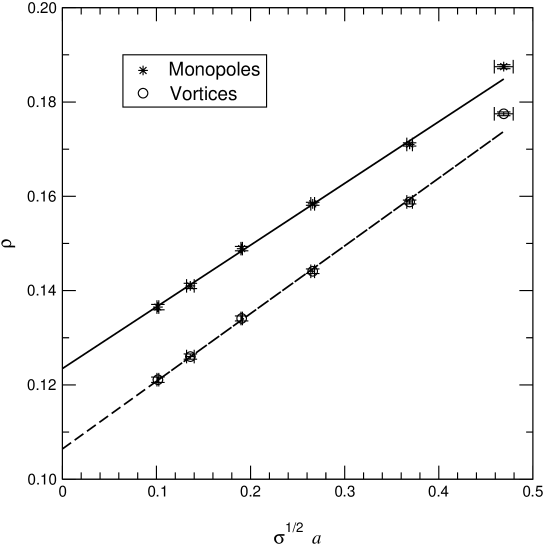
Figure 1: The dependence of $\rho$ on $a(\beta)$ for the Simple Center Vortices and the Simple Center Monopoles. The lattice has dimensions $24^{4}$. The lines are linear fits.

Figure 2: The Creutz ratio for the configurations for which there is no vortex inside the Wilson loops versus the size of the loop. The Creutz ratio for full SU(2) is given for comparison.

References

- [1] L. Streit, Functional Integrals for Quantum Theory, in H. Latal and W. Schweiger (Eds.), “Methods of Quantization”, Lecture Notes in Physics LNP 572, Springer-Verlag, (Berlin, Heidelberg 2001)
-
[2]
M.N. Chernodub, F.V. Gubarev, M.I. Polikarpov, and V.I. Zakharov,
Nucl. Phys. B 592 (2001) 107; hep-lat/0003138 - [3] V. Dzhunushaliev, D. Singleton, hep-th/9912194
- [4] F.Lenz, S.Woerlen, hep-th/0010099
-
[5]
B.L.G. Bakker, A.I. Veselov, and M.A. Zubkov,
Phys. Lett. B 502 (2001) 338; hep-lat/0011062 - [6] M. Faber, J. Greensite, and S. Olejnik, in “Confinement, Topology, and other Non-Perturbative Aspects of QCD”, NATO Advanced Research Workshop, Stara Lesna, Slovakia, 2002
-
[7]
M.I. Polikarpov, U.J. Wiese, and M.A. Zubkov,
Phys. Lett. B 309 (1993) 133 -
[8]
M.N. Chernodub, M.I. Polikarpov, A.I. Veselov, and M.A. Zubkov,
Nucl. Phys. Proc. Suppl. 73 (1999) 575; hep-lat/9809158. - [9] M. Creutz, Quarks, gluons and lattices, Cambridge University Press, (Cambridge, 1985).
-
[10]
J.Fingberg, U.Heller, F.Karsch,
hep-lat/9208012 -
[11]
B.B. Mandelbrot, “Fractals - Form, Chance and Dimension” (Freeman, San
Francisco, 1977)
D.A. Russel, J.D. Hanson, and E. Ott, Phys. Rev. Lett. 45, (1980), 1175
P. Grassberger and I. Procaccia Phys. Rev. Lett. 50 (1983), 346 -
[12]
M.I. Polikarpov Phys.Lett. B 236 (1990), 61;
T.L. Ivanenko, A.V. Pochinsky, and M.I.Polikarpov, Phys. Lett. B252 (1990), 631 - [13] V.G. Bornyakov, M.N. Chernodub, F.V. Gubarev, M.I. Polikarpov, T. Suzuki, A.I. Veselov, and V.I Zakharov, Anatomy of the lattice magnetic monopoles, hep-lat/0103032 and Phys. Lett. B., in press