Abstract

We consider the $SO(3)$ lattice gauge theory at weak coupling, in the Villain action. We exhibit an analytic path in coupling space showing the equivalence of the $SO(3)$ theory with $SU(2)$ summed over all twist sectors. This clarifies the “mysterious phase” of $SO(3)$. As order parameter, we consider the dual string tension or center vortex free energy, which we measure in $SO(3)$ using multicanonical Monte Carlo. This allows us to set the scale, indicating that ${\cal O}(700)^{4}$ lattices are necessary to probe the confined phase. We consider the relevance of our findings for confinement in other gauge groups with trivial center.

1 Motivation

Our main motivation for a numerical study of the $SO(3)$ gauge theory on the lattice is to clarify an apparent paradox.

On one hand, $SO(3)=SU(2)/Z_{2}$, so that the $SO(3)$ theory is an $SU(2)$ theory in the adjoint representation. On the lattice, the Yang-Mills action $-\frac{1}{4}\int d^{4}xF_{\mu\nu}^{2}$ can be obtained as the naive continuum limit of a plaquette action taken in any representation. In the usual Wilson action $\beta_{F}\sum_{P}(1-\frac{1}{2}{\rm Tr}_{F}U_{P})$, the trace of the plaquette matrix $U_{P}$ is taken in the fundamental representation. The $SO(3)$ theory corresponds to action $\beta_{A}\sum_{P}(1-\frac{1}{3}{\rm Tr}_{A}U_{P})$, with the trace taken in the adjoint representation. The universality of the continuum fixed point leads us to believe that the $SO(3)$ and $SU(2)$ theories are equivalent not just in the naive continuum limit, but also non-perturbatively. Thus, $SO(3)$ should confine (at low temperature $T<T_{c}$), just like $SU(2)$.

On the other hand, $Center(SO(3))={\bf 1}$. There is no center symmetry to break in the case of $SO(3)$. This means that the well-accepted connection between center symmetry breaking and the deconfinement transition [1] cannot apply. Another order parameter must be found. In the process, we may learn some general lesson about the gauge group structure necessary to sustain confinement.

Our attention will focus on topological excitations common to both $SU(2)$ and $SO(3)$: center vortices. Remarkably, a group with a trivial center may still support center vortices. A center vortex is a two-dimensional topological excitation. To prevent its action from diverging, it is a pure gauge at $r=\infty$, characterized by the gauge transformation $g(\theta)$ applied to the trivial vacuum. In $SU(N)$, the non-trivial topology comes from the possibility that $g(\theta+2\pi)=g(\theta)\exp(i\frac{2\pi}{N}k),k=0,..,N-1.$ The integer $k$ is the “twist”, defined mod $N$, and the Wilson loop at $r=\infty$ takes value $W(r=\infty)=g^{-1}(0)g(2\pi)=\exp(i\frac{2\pi}{N}k)$. Notice that both $W(r=\infty)$ and the gauge field $A_{\mu}(r=\infty,\theta)=g^{-1}(\theta)\partial_{\mu}g(\theta)$ are unchanged if $g(\theta)$ is multiplied by a $Z_{N}$ center element. This implies that our topological excitations are characterized by equivalence classes $SU(N)/Z_{N}$ of gauge transformations. Twist arises from the non-trivial mapping of the $r=\infty$ circle to these equivalence classes: $\Pi_{1}(SU(N)/Z_{N})=Z_{N}$. For a general non-Abelian gauge group $G$, center vortices exist if $\Pi_{1}(G/Center(G))\neq{\bf 1}$. Thus, both $SU(2)$ and $SO(3)$ admit center vortices.

One may also realize this fact by recalling that center vortices arise as local gauge singularities after center gauge fixing [2], where center gauge is just the Landau gauge in the adjoint representation: the gauge condition only makes use of the $SO(3)$ content of the gauge links, so that the gauge singularities only depend on the $SO(3)$ part.

2 Center vortices in $SU(2)$

The relevance of center vortices for confinement in $SU(2)$ has been studied numerically in two ways. One can fix the gauge to a maximal or Laplacian center gauge, where center vortices can be identified as gauge singularities [2] or as P-vortices [4] and center projection can be performed. One can also study center vortices in a gauge-invariant way via the ’t Hooft loop [3], since a ’t Hooft loop of contour ${\cal C}$ creates a fluctuating center vortex sheet bounded by ${\cal C}$ [5]. In the latter case, a ’t Hooft loop of maximal size $L_{\rho}\times L_{\sigma}$ is equivalent to enforcing twisted boundary conditions [3] in the orthogonal $\mu\nu$ plane. A simple way to see this is to observe that the twist matrices $\Omega_{\mu},\Omega_{\nu}$ satisfy (for $SU(2)$) $\Omega_{\mu}\Omega_{\nu}=-\Omega_{\nu}\Omega_{\mu}$. Therefore, a Wilson loop of size $L_{\mu}\times L_{\nu}$ picks up a factor $\Omega_{\mu}\Omega_{\nu}\Omega_{\mu}^{\dagger}\Omega_{\nu}^{\dagger}=-{\bf 1}$. In other words, twisted b.c. multiply the largest Wilson loop at “$r=\infty$” by a center element, precisely as a center vortex does: twisted b.c. ($tbc$) create one center vortex (mod $2$) as compared to periodic b.c. ($pbc$).

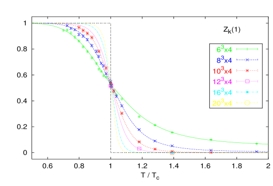
Figure 1.  : The effect of temporal twist in $SU(2)$: ratio $Z_{tbc}/Z_{pbc}$ as a function of temperature, for various lattice sizes (from [6]).

The ratio of partition functions $Z_{tbc}/Z_{pbc}=\exp(-F_{CV})$ probes the free energy $F_{CV}$ of a center vortex. Note that UV divergences cancel out in the ratio, so that it is a well-defined continuum quantity. On a hypercubic $L^{4}$ lattice, this ratio rapidly tends to $1$ as $L$ increases above $\sim 0.8$ fm [7]. At finite temperature, considering electric twist (i.e. in a temporal plane), this ratio is an order parameter for confinement [6]. Below $T_{c}$, the correlation length $\xi$ is finite and boundary conditions do not matter if the system size $L$ is $\gg\xi$: $Z_{tbc}/Z_{pbc}\rightarrow 1$. Above $T_{c}$, center vortices are “squeezed” by the compact Euclidean time. Their free energy increases as $\tilde{\sigma}(T)L^{2}$, generating an area law for the spatial ’t Hooft loop. The prefactor $\tilde{\sigma}(T)$ is the dual string tension, which varies with $T$ and vanishes as $T\rightarrow T_{c}^{+}$ with Ising-like critical exponents [8]. Since we claim to measure in $Z_{tbc}/Z_{pbc}$ a physical quantity, it should be measurable as well in the $SO(3)$ theory. We will see that this is indeed the case. $Z_{tbc}/Z_{pbc}$ is an order parameter also for $SO(3)$, and $\tilde{\sigma}(T)$ provides a way to measure the temperature also in that theory.

3 $SU(2)-SO(3)$ phase diagram and the $SO(3)$ “mysterious phase”

Contrary to the Wilson action $\beta_{F}\sum_{P}(1-\frac{1}{2}{\rm Tr}_{F}U_{P})$ which enjoys a smooth crossover from strong to weak coupling, the adjoint action $\beta_{A}\sum_{P}(1-\frac{1}{3}{\rm Tr}_{A}U_{P})$ produces a bulk, first-order phase transition at $\beta_{A}\approx 2.5$, which prevents an arbitrary decrease of $\beta_{A}$ while studying the weak coupling phase relevant for the continuum limit. The common wisdom is therefore that $SO(3)$ gives the same continuum physics as $SU(2)$, but that the lattice spacing is kept small by the necessity of staying on the weak coupling side of the bulk transition. One purpose of our study is to check this scenario. There is room for skepticism, because the phase diagram of a mixed $(\beta_{F},\beta_{A})$ action, first studied by Bhanot and Creutz [9], shows the weak coupling $\beta_{F}=0$ (i.e. $SO(3)$) phase qualitatively separated from the $SU(2)$ theory by a line of first-order phase transitions: there is no analytic $(\beta_{F},\beta_{A})$ path connecting the two. The possibility that the two theories are different has actually been proposed, with numerical results to support it, in [10].

Another feature of $SO(3)$ encouraging such speculation is the existence of a “mysterious phase”, reported by Datta and Gavai [11]. This phase appears in all respects similar to the “normal” phase, except for the Polyakov loop $P$: instead of $\frac{1}{2}{\rm Tr}_{F}P$ approaching $\pm 1$ as $\beta_{A}\rightarrow\infty$, it approaches zero (so that, in the adjoint representation, ${\rm Tr}_{A}P\rightarrow-1$ instead of $+3$). Tunneling between the two phases appears extremely infrequent, increasingly so at higher $\beta_{A}$. One wonders how the $SO(3)$ theory could have two distinct continuum limits, both similar to $SU(2)$.

To investigate this puzzle, we consider the Villain action for the $SO(3)$ theory, which associates a discrete variable $\alpha_{P}=\pm 1$ to each plaquette and has action $S=-\beta_{V}\sum_{P}\alpha_{P}\frac{1}{2}{\rm Tr}_{F}U_{P}$. Note that $\alpha_{P}$ can be integrated analytically, giving $S=-\sum_{P}\log\rm{cosh}(\frac{\beta_{V}}{2}{\rm Tr}_{F}U_{P})$, which is manifestly invariant under a change of sign of ${\rm Tr}_{F}U_{P}$, like the usual adjoint action $\beta_{A}\sum_{P}(1-\frac{1}{3}{\rm Tr}_{A}U_{P})=\frac{4}{3}\beta_{A}\sum_{P}(1-(\frac{1}{2}{\rm Tr}_{F}U_{P})^{2})$. Therefore, we deal with a genuine $SO(3)$ action, which shows the same bulk first-order transition (at $\beta_{V}\approx 4.47$) and the same “mysterious phase” [11]. The advantage of the Villain choice is that the connection $SO(3)\leftrightarrow SU(2)$ is easier to display.

4 Solving the puzzle: an analytic path between $SU(2)$ and $SO(3)$

This section contains no new results. We are simply pulling together observations previously made by various authors. Even the analytic path between $SO(3)$ and $SU(2)$ was already hinted at by Halliday and Schwimmer [12].

The first observation, originally due to Mack and Petkova [13], was made precise by Tomboulis and Kovacs [14]. The $SU(2)$ partition function for the Wilson action can be exactly rewritten as an $SO(3)$ partition function in Villain form, with the additional constraint that $\alpha_{P}$-monopoles are forbidden. Namely:

$$Z_{SU(2)}\equiv\int{\cal D}Ue^{\beta\sum_{P}{\rm Tr}_{F}U_{P}}\\ =c\!\!\sum_{\alpha_{P}=\pm 1}\int{\cal D}Ue^{\beta\sum_{P}\alpha_{P}{\rm Tr}_{F}U_{P}}\!\!\prod_{\rm{cubes}}\!\delta(\prod_{6}\alpha_{P}-1)$$ (1)

where $c$ comes from the normalization of the $\alpha_{P}$ integration.

The second observation is due to Alexandru and Haymaker [15], and is a refinement upon the first. While eq.(1) applies in an infinite volume, on a 4-torus one needs some additional global constraints on the $\alpha_{P}$ variables:

$$N_{\mu\nu}\equiv\prod_{P~{}\in~{}\rm{plane}~{}\mu\nu}\alpha_{P}=+1$$ (2)

for each product of $L_{\mu}\times L_{\nu}$ variables $\alpha_{P}$ in each $\mu\nu$ plane. Only configurations satisfying (2) can be mapped to $SU(2)$ configurations with periodic b.c. Note that, in the absence of $\alpha_{P}$-monopoles, $\prod_{P~{}\in~{}\rm{plane}~{}\mu\nu}\alpha_{P}$ is the same for every parallel plane $\mu\nu$. Therefore, eq.(2) defines 6 constraints only. If one imposes $N_{\mu\nu}=-1$ for some $\mu\nu$ orientation, then the mapping (1) is preserved, except that the $SU(2)$ b.c. are twisted in the $\mu\nu$ plane.

It is then straightforward to remove the constraints (2) by summing over all $2^{6}$ $N_{\mu\nu}$ possibilities. One obtains:

$$\sum_{\alpha_{P}=\pm 1}\int{\cal D}Ue^{\beta\sum_{P}\alpha_{P}{\rm Tr}_{F}U_{P}}\prod_{\rm{cubes}}\delta(\prod_{6}\alpha_{P}-1)=c^{-1}\!\!\!\sum_{\rm{all~{}twist~{}sectors}}\!\!\!Z_{SU(2)}$$ (3)

The $SO(3)$ Villain partition function, with monopoles removed, is just the sum of $SU(2)$ partition functions over all possible twisted b.c.

The “mysterious phase” then must be one (or more) of these twisted $SU(2)$ sectors. Indeed, one knows how to construct a so-called “twist-eater”, a groundstate with zero action and twisted b.c. [16]. Suppose $N_{xt}=-1$ is enforced through $\alpha_{P}=-1$ for all $xt$ plaquettes at $(1,y,z,1)$, $+1$ otherwise. Then, set all links to ${\bf 1}$, except $U_{x}(1,y,z,t)=i\sigma_{1}$ and $U_{t}(x,y,z,1)=i\sigma_{2}$. This choice yields $\frac{1}{2}{\rm Tr}_{F}U_{P}=+1$, except for $x=t=1$ in $xt$ planes, where $U_{P}=-{\bf 1}$. This minus sign cancels with that of $\alpha_{P}$ to give zero action. Note that the two Polyakov loops $P_{x}$ and $P_{t}$ in the $x$ and $t$ directions are now $i\sigma_{1}$ and $i\sigma_{2}$, satisfying ${\rm Tr}_{F}P=0$.

Therefore, we guess that, whenever the $SO(3)$ system is in the mysterious phase characterized by ${\rm Tr}_{F}P_{t}\sim 0$ (i.e. ${\rm Tr}_{A}P_{t}\sim-1$), twist in the $\alpha_{P}$ variables must be present in some of the temporal planes. This proves to be correct, as illustrated in Fig. 2, where we show the Monte Carlo history of ${\rm Tr}_{A}P_{t}$, accompanied by that of $k_{x,y,z}$, where

$$k_{x}\equiv\frac{1}{2}\biggl{(}1-\frac{1}{L_{y}L_{z}}\sum^{L_{y}L_{z}}N_{xt}\biggr{)}$$ (4)

is the average, mapped to the interval $[0,1]$, of the $\alpha_{P}$-twist $N_{xt}$ in each $xt$ plane. This averaging is necessary because our $SO(3)$ action does not forbid $\alpha_{P}$-monopoles. They have a small ($\propto e^{-m\beta}$) density, which allows $N_{xt}=\prod_{P}\alpha_{P}$ to fluctuate from one parallel plane to another, so that $k_{x,y,z}$ fluctuate near $0$ or near $1$. Note also the very slow Monte Carlo dynamics, which prevent an ergodic sampling of configuration space on all but the smallest lattice sizes unless one resorts to special strategies, see sec. 5.

By measuring Polyakov loops in other directions, one can resolve whether one or more of the $k_{x,y,z}$ are near 1, and obtain a one-to-one mapping between Polyakov loops and twist sectors [17].

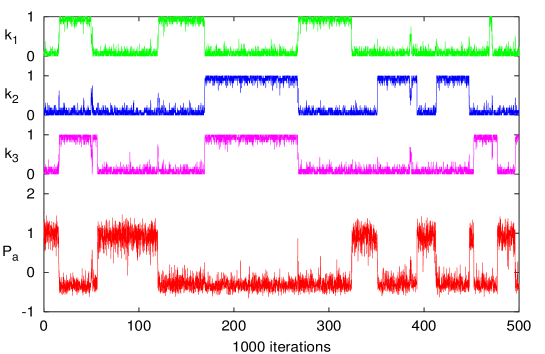
Figure 2.  : Monte Carlo history of the adjoint Polyakov loop (bottom) and of the 3 electric twist variables (top). The trace of the adjoint Polyakov loop is negative whenever twist is present ($4^{4}$ lattice, $\beta=4.5$).

Completing an analytic path between $SO(3)$ and $SU(2)$ requires one last, simple step. We need to allow again $\alpha_{P}$-monopoles, which can be done via a chemical potential $\lambda$, giving the partition function

$$Z=\sum_{\alpha_{P}=\pm 1}\int{\cal D}U\exp\Bigl{(}\beta\sum_{P}\alpha_{P}{\rm Tr}_{F}U_{P}+\lambda\sum_{\rm{cubes}}\prod_{6}\alpha_{P}\Bigr{)}$$ (5)

In the limit $\lambda\rightarrow+\infty$, $\alpha_{P}$-monopoles are forbidden and eq.(3) holds. The $SO(3)$ Villain action which we study corresponds to $\lambda=0$. The phase diagram in the $(\lambda,\beta)$ coupling plane has been studied in [11]. We reproduce it in Fig. 3. At strong coupling, monopoles condense: their density is ${\cal O}(1)$, which introduces strong fluctuations in $\prod_{P}\alpha_{P}$ from one parallel plane to another. Variables $k_{x,y,z}$ fluctuate around $\frac{1}{2}$, and the concept of twist is ill-defined. On the other hand, at weak coupling, monopoles are exponentially suppressed, long-range order appears among the $\alpha_{P}$ variables, and twist sectors become well-defined. There is no non-analyticity between $(\lambda=0,\beta>\beta_{c}\approx 4.47)$, which is the weak-coupling $SO(3)$ Villain theory under study, and $\lambda=+\infty$, which is equivalent to $SU(2)$ summed over all twist sectors as per eq.(3). Therefore, the non-perturbative continuum physics of $SO(3)$ is the same as that of $SU(2)$, summed over all twist sectors.

What remains to do is to put this statement on a quantitative footing, by matching the lattice spacings $a(\beta)$ in $SO(3)$ and $SU(2)$. We accomplish this next by measuring the dual string tension $\tilde{\sigma}(T)$ in both theories.

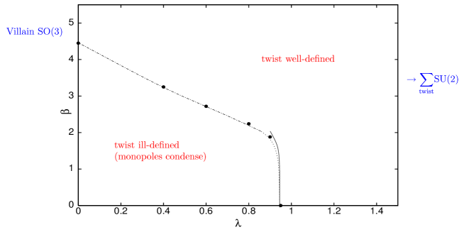
Figure 3.  : Phase diagram in the coupling plane $(\lambda,\beta)$, where $\lambda$ is the monopole chemical potential and $\beta$ the $SO(3)$ gauge coupling (adapted from Ref.[11]).

5 The order parameter and its measurement

Defining an order parameter for confinement in $SO(3)$ is not a trivial matter, as emphasized by Smilga [18]. The trace of the $SU(2)$ Polyakov loop, like that of all Wilson loops, is identically zero in the fundamental representation. In the adjoint representation, the trace of the Polyakov loop is always non-zero, since adjoint charges are screened by gluons at any temperature. Here, we use the dual string tension $\tilde{\sigma}(T)$, which is zero in the confining phase $T<T_{c}$, positive and increasing with $T$ in the deconfined phase $T>T_{c}$, and which we already showed to be a good order parameter in the $SU(2)$ theory (see [8, 6] and Fig. 1).

In $SU(2)$, on a lattice of physical size $L^{3}\times T^{-1}$, the dual string tension can be obtained from the ratio of twisted (in a temporal $L\times T^{-1}$ plane) and periodic partition functions:

$$\tilde{\sigma}(T)=\lim_{L\rightarrow\infty}-(1/L^{2})\log Z_{tbc}/Z_{pbc}$$ (6)

The presence or absence of twist is imposed by hand, by a specific choice of boundary conditions. In $SO(3)$, twist sectors are automatically summed over, and twist becomes an observable, similar to the usual topological charge in $SU(2)$. Sectors of different twist, which would be disjoint in the continuum limit, are connected at finite $\beta$ via saddle points which are lattice artifacts, analogous to topological “dislocations”. The assignment of an integer twist (in each plane) to a given configuration is subject to ambiguities similar to the assignment of a topological charge. Fortunately, we work at a very weak coupling, so that such ambiguities have a negligible impact in our case: the twist variables $k_{x,y,z}$ (eq.(4)) stay near $0$ or $1$. The price we have to pay is that the twist sectors are separated by very high action barriers $\Delta S$, nearly impassable for an ordinary Monte Carlo algorithm.

     

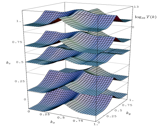
Figure 4.  : The three-dimensional reweighting table used in our multicanonical Monte Carlo. No twist is at bottom left, twist in all 3 planes at top right. The table enhances the probability of sampling the saddles between twist sectors. Its entries vary by 13 orders of magnitude ($8^{3}\times 4$ lattice, $\beta=4.5$).

Our strategy to solve this technical problem is multicanonical sampling [19]. Instead of assigning probability $\frac{1}{Z}e^{-S}$ to each configuration, we multiply this probability by a factor $T(k)$ which favors the saddle points between twist sectors $k\sim 0$ and $k\sim 1$, tuned such that the resulting sampling probability is flat from one sector to the next. The Monte Carlo process then amounts to a free diffusion across twist sectors, with dynamics accelerated exponentially (by a factor $\sim e^{\beta\Delta S}$).

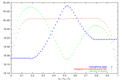
Figure 5.  : Cut of the three-dimensional reweighting table along its diagonal (blue *). The result of multicanonical Monte Carlo sampling is a nearly flat histogram (red +). The density of states shows the dominant twist-0 and the smaller twist-3 sectors (green x).

In our case, we want to facilitate the Monte Carlo sampling of twist in all 3 temporal planes. This leads us to a multicanonical sampling with a 3-dimensional reweighting factor $T(k_{x},k_{y},k_{z})$ which can be represented by a table since $k_{x,y,z}=\hat{k}/L^{2}$, $\hat{k}=[0,..,L^{2}]$. This table is constructed iteratively, using converged values on small lattices to form starting values on larger ones. Such a table is displayed in Fig. 4, for an $8^{3}\times 4$ lattice at $\beta=4.5$. Although $\beta$ has been chosen as small as possible (the bulk transition to the strongly coupled phase occurs at $\beta_{c}\approx 4.47$), the necessary enhancement of the saddle points reaches $10^{13}$, as seen more clearly in Fig. 5, which is a $1d$-cut of the same table along its diagonal (from $k_{x,y,z}=(0,0,0)$ to $(1,1,1)$). There, the resulting flatness of the Monte Carlo sampling probability is clearly visible. The measured density of states shows two well-separated peaks, corresponding to twist sectors $(0,0,0)$ (analogous to $SU(2)~{}pbc$) and $(1,1,1)$ (analogous to $SU(2)~{}tbc$ in all 3 temporal planes). The strong suppression of the saddle point confirms that ordinary Monte Carlo sampling would remain hopelessly “stuck” in one sector, as observed in earlier studies. However, in spite of the great multicanonical acceleration, the Monte Carlo evolution of the twist variables $k_{x,y,z}$ is still slow, and simulating a $10^{3}\times 4$ lattice remains beyond the edge of our computer resources.

This prevents us from reaching spatial sizes large enough for a reliable extrapolation of eq.(6) to $L\rightarrow\infty$. Our extrapolation depends on the ansatz we choose for the finite-size effects. Nevertheless, we can still calibrate the $SO(3)$ lattice spacing $a(\beta_{SO(3)}=4.5)$, by comparing our $L=4,6,8$ results with those obtained in $SU(2)$ on the same lattice sizes $L^{3}\times 4$. In both theories, our observables are $Z_{tbc}^{k}/Z_{pbc}\equiv\exp(-F_{CV}^{k})$, where $k=1,2,3$ refers to twisted b.c. in 1, 2 or 3 temporal planes. In $SO(3)$, these observables are obtained from the Monte Carlo distribution of the twist variables $k_{x,y,z}$. This distribution falls into $2^{3}$ distinct, well-separated peaks, as in Fig. 5, and we measure the ratio of the population around each peak to that around the $pbc$ peak at $k_{x,y,z}\sim 0$. In $SU(2)$, these ratios are obtained from different Monte Carlo simulations, following the method of [8].

     

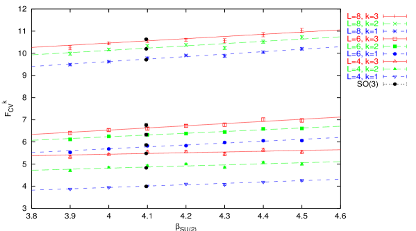
Figure 6.  : Comparison of the twist free energies between $SO(3)$ at $\beta=4.5$ and $SU(2)$ at various $\beta$’s. Electric twist in 1, 2 and 3 planes is considered, on lattices of size $4^{3},6^{3}$ and $8^{3}\times 4$. One finds $\beta_{SO(3)}=4.5\longleftrightarrow\beta_{SU(2)}=4.10(15)$.

The twisted free energies $F_{CV}^{k}$ are continuum quantities, which depend upon the spatial size $L$ and the temperature $T$. If the $SO(3)$ and $SU(2)$ theories represent the same continuum physics, then to each $\beta_{SO(3)}$ should correspond a value $\beta_{SU(2)}$, which yields the same lattice spacing and thereby the same $F_{CV}^{k}$ for equal lattice sizes, modulo small lattice artifacts. We test this statement in Fig. 6. The 9 free energies $F_{CV}^{k},k=1,2,3$ measured on $4^{3},6^{3}$ and $8^{3}\times 4$ lattices in $SO(3)$ at $\beta_{SO(3)}=4.5$ are compared with similar quantities measured in $SU(2)$ at different values of $\beta_{SU(2)}$. The straight lines show a linear interpolation in $\beta_{SU(2)}$ of the $SU(2)$ data. One observes a very good match of all 9 observables, for $\beta_{SU(2)}\approx 4.10(15)$.

Thus, $a^{-1}(\beta_{SO(3)}=4.5)\approx a^{-1}(\beta_{SU(2)}=4.1)$, which is about $200$ GeV! As conventional wisdom asserts, our $SO(3)$ lattice is very fine indeed. To reach low temperatures $T<T_{c}$ and probe the confined phase would require a lattice of size ${\cal O}(700)^{4}$, far beyond what is currently achievable.

Note the closeness of the matched $SO(3)$–$SU(2)$ bare couplings ($\frac{4}{g^{2}}=4.5$ vs $4.1$). This should come as no surprise. Lattice perturbation theory is identical between the $SU(2)$ Wilson action and the $SO(3)$ Villain action: the difference resides in the $\alpha_{P}$-monopoles, which do not appear in the perturbative expansion. Therefore, $\Lambda_{\rm{lattice}}$ is the same in both theories, and one should expect similar values for the non-perturbatively matched $\beta$’s. The $\alpha_{P}$-monopoles disorder the $SO(3)$ theory slightly, which is why the matching $SU(2)$ $\beta$ is slightly smaller.

6 Conclusion

To summarize, conventional wisdom prevails and there is no mystery. The $SO(3)$ lattice theory at weak coupling gives the same non-perturbative physics as the $SU(2)$ theory and a common confinement order parameter exists for both: the center vortex – or twist – free energy. The difference is that a definite twist sector is selected via the choice of boundary conditions in $SU(2)$, whereas all sectors are automatically summed over in $SO(3)$.

Unfortunately, the numerical study of the $SO(3)$ theory seems limited to very fine lattice spacings, because a bulk transition prevents exploring continuum physics at stronger bare couplings. One way out is to suppress the formation of monopoles whose condensation triggers the bulk transition [20]. However, this appealing approach suffers from an unpleasant, technical side-effect. The Monte Carlo sampling over the various twist sectors, which is essential to measure the confinement order parameter, is made more difficult by higher action barriers separating the sectors. This situation is analogous to simulations of overlap or domain-wall fermions. There, dislocations separating topological sectors cause trouble in the inversion of the Dirac operator. They can be suppressed by choosing a gauge action which assigns them a large action. The price to pay is a much slower Monte Carlo evolution of the topological charge. One may hope that a clever enhancement of the sampling probability in the neighborhood of the saddle point, and only there, as in [21], can solve both types of problems.

Finally, one can try to generalize the lesson learnt here about the structure of the gauge group $G$ necessary for confinement. $SO(3)$ shows that a non-trivial center is not required. On the other hand, the existence of the dual string tension arises from that of the twist sectors. Those in turn follow from the non-trivial first homotopy group $\Pi_{1}(G/Center(G))$, which is the same for $SU(2)$ and $SO(3)$. A non-trivial $\Pi_{1}(G/Center(G))$, or more precisely $\Pi_{1}(G/Z_{G})$, where $Z_{G}$ is the discrete part of the center of $G$, is necessary for a dual string tension to be defined. The non-trivial elements of this group are the center vortex (or twist) excitations. Therefore, we conjecture that the existence of center vortices is a necessary condition for the existence of an ordinary string tension, i.e. for confinement. It is not a sufficient condition: compact $U(1)$ has twist sectors but its weak-coupling phase does not confine. On the other hand, there are non-Abelian Lie groups which do not meet this condition, namely $G_{2}$, $F_{4}$ and $E_{8}$. Therefore, we conjecture that these cannot confine (in the sense that the Wilson loop cannot obey an area law).

7 Acknowledgements

We are grateful to G. Burgio, M. Müller-Preussker and L. von Smekal for discussions. We thank the conference organizers for their talent in creating a stimulating atmosphere and their patience in awaiting this manuscript.

References

- [1] Svetitsky, B. and Yaffe, L.G. (1982) Critical Behavior At Finite Temperature Confinement Transitions, Nucl. Phys., B210, pp. 423
- [2] de Forcrand, Ph. and Pepe, M. (2001) Center vortices and monopoles without lattice Gribov copies, Nucl. Phys., B598, pp. 557
- [3] ’t Hooft, G. (1978) On The Phase Transition Towards Permanent Quark Confinement, Nucl. Phys., B138, pp. 1; ’t Hooft, G. (1979) A Property Of Electric And Magnetic Flux In Nonabelian Gauge Theories, Nucl. Phys., B153, pp. 141
- [4] Del Debbio, L., Faber, M., Greensite, J. and Olejnik, Š. (1997) Center dominance and Z(2) vortices in SU(2) lattice gauge theory, Phys. Rev., D 55, pp. 2298
- [5] de Forcrand, Ph. and von Smekal, L. (2002) ’t Hooft loops and consistent order parameters for confinement, Nucl. Phys. Proc. Suppl., 106, pp. 619
- [6] de Forcrand, Ph. and von Smekal, L. (2001) ’t Hooft loops, electric flux sectors and confinement in SU(2) Yang-Mills theory, hep-lat/0107018
- [7] Kovács, T.G. and Tomboulis, E.T. (2000) Computation of the vortex free energy in SU(2) gauge theory, Phys. Rev. Lett., 85, pp. 704
- [8] de Forcrand Ph., D’Elia, M. and Pepe, M. (2001) A study of the ’t Hooft loop in SU(2) Yang-Mills theory, Phys. Rev. Lett., 86, pp. 1438
- [9] Bhanot, G. and Creutz, M. (1981) Variant Actions And Phase Structure In Lattice Gauge Theory, Phys. Rev., D24, pp. 3212
- [10] Langfeld, K. and Reinhardt, H. (2000) The Stefan-Boltzmann law: SU(2) versus SO(3) lattice gauge theory, hep-lat/0001009
- [11] Cheluvaraja, S. and Sharathchandra, H.S. (1996) Finite temperature properties of mixed action lattice gauge theory, hep-lat/9611001; Datta, S. and Gavai, R.V. (1998) Phase transitions in SO(3) lattice gauge theory, Phys. Rev., D57, pp. 6618
- [12] Halliday, G. and Schwimmer, A. (1981) Z(2) Monopoles In Lattice Gauge Theories, Phys. Lett., B102, pp. 337
- [13] Mack, G. and Petkova, V.B. (1982) Z2 Monopoles In The Standard SU(2) Lattice Gauge Theory Model, Z. Phys., C12, pp. 177
- [14] Tomboulis, E. (1981) The ’T Hooft Loop In SU(2) Lattice Gauge Theories, Phys. Rev., D23, pp. 2371; Kovács, T.G. and Tomboulis, E.T. (1998) Vortices and confinement at weak coupling, Phys. Rev., D57, pp. 4054
- [15] Alexandru, A. and Haymaker, R.W. (2000) Vortices in SO(3) x Z(2) simulations, Phys. Rev., D62, pp. 074509
- [16] Ambjørn, J. and Flyvbjerg, H. (1980) ’t Hooft’s nonabelian magnetic flux has zero classical energy, Phys. Lett., B97, 241; Groeneveld, J., Jurkiewicz, J. and Korthals Altes, C.P. (1981) Twist as a probe for phase structure, Phys. Scripta, 23, 1022
- [17] de Forcrand, Ph. and Jahn, O., in writing.
- [18] Smilga, A.V. (1994) Are Z(N) Bubbles Really There?, Annals Phys., 234, pp. 1
- [19] Berg, B.A. and Neuhaus, T. (1991) Multicanonical Algorithms For First Order Phase Transitions, Phys. Lett., B267, pp. 249
- [20] Barresi, A., Burgio, G. and Müller-Preussker, M. (2002) Finite temperature phase transition, adjoint Polyakov loop and topology in SU(2) LGT, Nucl. Phys. Proc. Suppl., 106, pp. 495
- [21] de Forcrand, Ph., Hetrick, J.E., Takaishi, T. and van der Sijs, A. (1998) Three topics in the Schwinger model, Nucl. Phys. Proc. Suppl., 63, pp. 679