Lattice QCD with Suppressed High Momentum Modes of the Dirac Operator

Abstract.

I define lattice fermions in five Euclidean dimensions and the corresponding effective theory in four dimensions. The main properties of these theories include the suppression of high momentum modes of the lattice Dirac operator and their ability to continuously interpolate between quenched and dynamical fermions. In particular, the standard formulation of lattice QCD can be viewed as a limiting case of the theory.

Lattice simulations are an indispensable tool in understanding the strong force. Since its formulation by [Wilson, 1974], lattice Quantum Chromodynamics (QCD) has progressed into a separate discipline.

Nevertheless, simulations of lattice QCD are still away form the precision tests that one would like to see. Clearly, faster computers and simulation algorithms are needed.

Recently, the issue of ‘ultraviolet (UV) slowing down’ has attracted particular interest [Irving et al, 1998, Duncan, Eichten and Thacker, 1999, de Forcrand, 1999, Peardon, 2001, A. Hasenfratz & Knechtli, 2001]. These studies try to address algortmically large fluctuations of the high end modes of the fermion determinant. The goal of these algorithms is to separate the UV modes and to focus on the silumation of the physically interesting infrared modes. In this paper I show that all this computational effort can be saved if one improves UV properties of the lattice Dirac operator in the first place.

Much of UV slowing down is thought to come from the non-smoothness of the gauge fields [A. Hasenfratz & Knechtli, 2001]. The effects of non-smooth gauge fields are mostly observed in the large eigenvalues of the fermion determinant [Irving et al, 1998]. Recently, [Duncan, Eichten and Thacker, 1999] proposed a strategy to accelerate fermion simulations by computing directly the ‘infrared’ eigenvalues and attaching the ‘ultraviolet’ ones by approximate actions and the multiboson method. [de Forcrand, 1999] proposed an algorithm which ‘filters’ these fermion modes. Another strategy is the inclusion of ultraviolet modes in a multibosonic fashion which results in faster algorithms [Peardon, 2001]. A direct smoothing approach is also possible by smearing techniques [A. Hasenfratz & Knechtli, 2001].

In spite of the recent progress there is no unifying view how to deal with the UV slowing down. In this paper I propose an improved formulation of lattice fermions which ‘quenches’ fermion eigenvalues beyond a given eigenvalue level. The paper proves rigorously the existence of such a field theory.

In the following section I discuss the need to deal with the problem of non-smooth lattice gauge fields. In section 2 I give a model of five dimensional fermions with suppressed high fermion modes. I then define the theory in four dimensions and prove its the field theoretic properties in section 3. Finally, in section 4 I draw the conclusions.

1. Difficulties with lattice fermions

1.1. Basic definitions

The lattice regularization of gauge theories was defined by [Wilson, 1974].

A fermion field on a regular Euclidean lattice $\Lambda$ is a Grassmann valued vector $\psi(x),~{}~{}~{}x=\{x_{\mu},\mu=1,\ldots,4\}\in\Lambda$ which carries spin and color indices. The first and second order differences are defined by the following expressions:

$$\begin{array}[]{l}{\hat{\partial}}_{\mu}\psi(x)=\frac{1}{2a}[\psi(x+ae_{\mu})-\psi(x-ae_{\mu})]\\ \\ {\hat{\partial}}_{\mu}^{2}\psi(x)=\frac{1}{~{}~{}~{}~{}a^{2}}[\psi(x+ae_{\mu})+\psi(x-ae_{\mu})-2\psi(x)]\end{array}$$

where $a$ and $e_{\mu}$ are the lattice spacing and the unit lattice vector along the coordinate $\mu=1,\ldots,4$. Let $U(x)_{\mu}\in\mathbb{C}^{3\times 3}$ be an element of the $SU(3)$ group, the oriented link connecting lattice sites $x$ and $x+ae_{\mu}$. Then covariant differences are defined by:

$$\begin{array}[]{l}\nabla_{\mu}\psi(x)=\frac{1}{2a}[U(x)_{\mu}\psi(x+ae_{\mu})-U^{{\dagger}}(x-ae_{\mu})_{\mu}\psi(x-ae_{\mu})]\\ \\ \Delta_{\mu}\psi(x)=\frac{1}{~{}~{}~{}~{}a^{2}}[U(x)_{\mu}\psi(x+ae_{\mu})+U^{{\dagger}}(x-ae_{\mu})_{\mu}\psi(x-ae_{\mu})-2\psi(x)]\end{array}$$

The Wilson-Dirac operator is a matrix operator $D_{W}\in\mathbb{C}^{N\times N}$ defined by:

(1.1) $$D_{W}=m\text{1\kern-2.41109ptl}+\sum_{\mu=1}^{4}(\gamma_{\mu}\nabla_{\mu}-\frac{a}{2}\Delta_{\mu})$$

where 1l is the identity matrix and $m$ the bare mass of the fermion; $\{\gamma_{\mu}\in\mathbb{C}^{4\times 4},\mu=1,\ldots,4\}$ is the set of anti-commuting and Hermitian gamma-matrices of the Dirac-Clifford algebra. The fermion lattice action is defined by:

(1.2) $$S_{f}=\sum_{x,y\in\Lambda}{\bar{\psi}}(x)D_{W}(x,y)\psi(y)$$

whereas the gauge action is given by:

(1.3) $$S_{g}=\frac{1}{g^{2}}\sum_{\mathbb{P}}(\text{1\kern-2.41109ptl}-U_{\mathbb{P}})$$

The sum in the right hand side is over all plaquettes $\mathbb{P}$ on the lattice. $U_{\mathbb{P}}$ is $1\times 1$ Wilson loop and $g$ is the bare coupling constant of the theory.

The basic computational task in lattice QCD is the evaluation of the partition function given by:

(1.4) $$Z_{QCD}=\int\sigma_{H}(U)\sigma(\psi,{\bar{\psi}})e^{-S_{f}-S_{g}}$$

where $\sigma_{H}(U)$ and $\sigma(\psi,{\bar{\psi}})$ denote the Haar and Grassmann measures respectively. The computing problem has $O(e^{N})$ complexity (i.e. it is NP-hard) and one has to resort to stochastic estimations of the right hand side (1.4). In fact, integration over the Grassmann fields can be performed exactly to give:

$$Z_{QCD}=\int\sigma_{H}(U)\det D_{W}e^{-S_{g}}$$

1.2. A measure of non-smoothness of lattice gauge fields

I will use a linear function of plaquette to characterize the degree of the non-smoothness on the lattice. Let $P(U)$ be the average $1\times 1$ Wilson loop over all lattice plaquettes. Then I define the following real and positive function:

(1.5) $$\Phi(U)=1-P(U)=1-\langle U_{\mathbb{P}}\rangle_{\mathbb{P}}$$

Smooth gauge fields are characterized by small values of $\Phi(U)$. Typical values from lattice simulations are $\Phi(U)\in(0.4,0.5)$, which is a clear indication of non-smoothness of the lattice gauge fields.

To see the influence of the non-smoothness on a typical gauge invariant lattice operator, I consider eigenvalue perturbations of the lattice Dirac operator. Let $\lambda(U)$ be an eigenvalue of the matrix $A(U)\equiv D_{W}^{{\dagger}}D_{W}$. A classical result from the eigenvalue perturbation theory states that variation of an eigenvalue $\delta\lambda(U)$ under matrix perturbation $\delta A(U)$ is bounded by [Golub & Van Loan, 1989]:

(1.6) $$\left|\delta\lambda(U)\right|\leq\left\|\delta A(U)\right\|_{p},~{}~{}~{}~{}~{}p\in\mathbb{N}$$

The following result relates the 2-norm of the matrix $A(U)$ to the degree of the non-smoothness $\Phi(U)$ on the lattice (1.5):

(1.7) $$\left\|\delta A(U)\right\|_{2}\leq c_{1}+c_{2}\sqrt{\Phi(U)}$$

where $c_{1}$ and $c_{2}$ are positive constants. This result is proven in Appendix A. Together with the bound (1.6) it gives:

(1.8) $$\left|\delta\lambda(U)\right|\leq c_{1}+c_{2}\sqrt{\Phi(U)}$$

The above inequality (1.8) states that the eigenvalue fluctuations on a lattice with smooth gauge fields are likely to be smaller than those on a lattice with non-smooth gauge fields.

However, as present computing resources do not allow a close approach to continuum limit, it is important to look for formulations and algorithms with reduced effects of lattice non-smoothness.

Numerical results of [Duncan, Eichten and Thacker, 1999] indicate that large eigenvalues of the lattice Dirac operator are merely lattice artifacts. It is a well-known fact that cutoff modes are poorly represented on the lattice. But one may not simply exclude them from simulations since the existence of the theory may be compromised. The strategy followed in this paper is the suppression of the high fermion modes of the lattice theory. As shown below it is possible to model a fermion theory with the reduced appearance of these modes.

2. Modeling cutoff modes: Wilson fermions in 4$+$1 Euclidean dimensions

Recent progress with chiral fermions on the lattice has shown that a theory of five dimensional fermions can be a useful modeling tool (for a review see [Kikukawa, 2001]). Domain wall boundary conditions along the fifth dimension provide a kinematical model for QCD with chiral fermions which are “localized” on the surface of a five dimensional world. The theory in five dimensions can be viewed as a fermion system propagating along the fifth Euclidean dimension with its dynamics generated by a certain Hamiltonian operator $\mathcal{H}$.

Let $c^{{\dagger}}(x)$ and $c(x)$ be creation and destruction operators in the Fock space which satisfy the anti-commutation relations:

$$[c^{{\dagger}}(x),c(x)]_{+}=\text{1\kern-2.41109ptl}$$

They carry spin and color indices, which are not explicitly shown for clarity. $c(x)$ acts on the bare vacuum state which they annihilate.

I define the Hamiltonian operator of the fermion system by the bilinear form:

$$\mathcal{H}=\sum_{x,y\in\Lambda}c^{{\dagger}}(x)H_{W}(x,y)c(y)$$

where $H_{W}$ is the Hermitian lattice Dirac operator in four dimensions given by:

$$H_{W}=\gamma_{5}D_{W}$$

Let $L_{5}$ be the lattice size in the fifth dimension or the “the inverse temperature” of the quantum statistical system with the partition function $Z$, given by:

$$Z=\text{Tr}~{}~{}e^{-L_{5}\mathcal{H}}$$

To compute the trace of an operator in the Fock space I use the standard technique of the Grassmann coherent states with antiperiodic boundary conditions in the fifth Euclidean coordinate. Since $\mathcal{H}$ is quadratic it is easy to show that:

$$Z=\det(\text{1\kern-2.41109ptl}+e^{-L_{5}H_{W}})$$

I define the measure density of the non-trivial fermion theory on the lattice by the following equation:

$$\omega(H_{W})=\frac{1}{Z}\text{Tr}~{}~{}\mathcal{O}e^{-L_{5}\mathcal{H}}$$

where $\mathcal{O}$ is a function of the creation and annihilation operators. I choose it such that the right hand side is given by:

$$\omega(H_{W})=\frac{1}{Z}\det(\text{1\kern-2.41109ptl}-e^{-L_{5}H_{W}})$$

Such an operator exists as it is shown in the framework of domain wall fermions [Furman, Shamir, 1995].

Hence the resulting density can be written as:

(2.1) $$\omega(H_{W})=\det(\tanh\frac{L_{5}}{2}H_{W})$$

This suggests that an effective theory in four dimensions may be defined by the following lattice Dirac operator:

(2.2) $$D=\frac{\mu}{a}\gamma_{5}\tanh\frac{aH_{W}}{\mu}$$

where $a$ is the lattice spacing of the four dimensional lattice and $\mu>0$ is a dimensionless parameter. It is clear that for small lattice spacing this operator approaches the Wilson Dirac operator and hence has the correct continuum limit.

In order to give to the Tr$~{}~{}\mathcal{O}$ operator a precise meaning, I define a fermion theory in five dimensions by the following action:

(2.3) $$S^{(5)}={\bar{\psi}}^{(5)}D_{W}^{(5)}\psi^{(5)}$$

Here the five dimensional fermion field $\psi^{(5)}$ satisfies periodic boundary conditions in all directions and $D_{W}^{(5)}$ is defined by:

$$D_{W}^{(5)}=D_{W}+\gamma_{5}\nabla_{5}-\frac{a_{5}}{2}\Delta_{5}$$

It can be shown that: The measure density of the five dimensional theory (2.3) is proportional to the measure of the effective theory defined by eq. (2.1). The proof is given in Appendix B.

This result suggests that the four dimensional lattice theory with Wilson fermions can be approached by the ‘high temperature’ limit of a theory with Wilson fermions in five dimensions. Thus, it is natural to choose the length of the extra dimension to be proportional to the lattice spacing in four dimensions. Dimensional reduction is then realized by taking the continuum limit of the theory. Furthermore, the theory allows the introduction of a dimensionless parameter $\mu$ which can be used to suppress the high momentum modes of the fermion theory to a prescribed level, i.e. $\mu$ can be viewed as a dimensionless ‘temperature’. A ‘cold’ theory would then correspond to the quenched approximation, whereas a ‘hot’ one would be identical to the Wilson theory.

In the next section I will give the basic properties of the dimensionally reduced effective theory.

3. A fermion theory with suppressed cutoff modes

It is clear that the above theory defined in 4$+$1 dimensions has all desired properties of a field theory: it is local, unitary and gauge invariant.

This is not obvious for the dimensionally reduced theory with a lattice Dirac operator given by (2.2):

(3.1) $$D=\frac{\mu}{a}\gamma_{5}\tanh\frac{aH_{W}}{\mu}$$

For free fermions the lattice Dirac operator has a momentum space representation given by:

(3.2) $${\tilde{D}}(p)=\frac{\mu}{a}\gamma_{5}\tanh\frac{a{\tilde{H}_{W}}(p)}{\mu}$$

with $p=\{p_{\nu},\nu=1,\ldots,4\}$ being the four-momentum vector. The momentum space Wilson Dirac operator is given by:

$${\tilde{D}}_{W}(p)=\frac{1}{a}\sum_{\nu=1}^{4}(\text{1\kern-2.41109ptl}-e^{-i\gamma_{\nu}ap_{\nu}})$$

whereas its square is given by:

$$a^{2}{\tilde{D}}_{W}(p)^{{\dagger}}{\tilde{D}}_{W}(p)=\sum_{\nu=1}^{4}\sin^{2}ap_{\nu}+[\sum_{\nu=1}^{4}(1-\cos^{2}ap_{\nu})]^{2}$$

3.1. Locality

Whilst $D_{W}$ links only nearest neighbour lattice points, $D$ will be a full matrix. A full matrix can be considered essentially local if it is dominated by matrix elements which link lattice points that are close to each other. For example, this will be the case if the magnitude of $D_{ij}$ decays exponentially with the distance $|i-j|$. This will be considered as a sufficient condition in the following for locality (see also [Hernández et al, 1999]). Since ${\tilde{D}}(p)$ is analytic and $2\pi$-periodic for $\mu>0$, then its Fourier transform falls off exponentially at large distances (see [Lüscher, 1998] for a similar argument). Therefore, $D$ is a local operator in the above sense.

The locality of the fermion theory in a gauge field background is treated in Appendix C. In particular, it is shown that if the Wilson Dirac operator is singular the locality of the theory is guaranteed solely by the positivity of $\mu$.

3.2. Unitarity

For unitarity it is sufficient to show that the lattice operator leads to non-negative energy spectrum with non-negative norm of eigenmodes. To do this I define a positive function $\tilde{f}$ in terms of the real variable $z$:

$${\tilde{f}}(z)=\frac{1}{z}\tanh z,~{}~{}~{}~{}z\neq 0$$

Since $\tanh z$ is an odd function of $z$, one can easily show that the right hand side is in fact a function of $z^{2}$ only. Therefore, I can define a function $f$ such that:

(3.3) $$\begin{array}[]{l}f(z^{2})=\frac{1}{z}\tanh z,~{}~{}~{}~{}z\neq 0\\ f(0)=1\end{array}$$

This way, I may write:

$$\tanh z=zf(z^{2}),~{}~{}~{}~{}z\in\text{I\kern-1.80832ptR}$$

Using the definition of an operator-valued function the lattice Dirac operator (2.2) takes the form:

(3.4) $$D=D_{W}f[(\frac{aH_{W}}{\mu})^{2}]$$

Now note that the matrix function $f(.)$ is non-singular. Hence the poles in the fermion propagator are identical to those in the Wilson theory and the resulting theory is characterized by a real energy spectrum. Moreover, since $f(.)$ is positive definite the norm of energy eigenmodes remains positive.

3.3. Perturbation theory

The fermion propagator is given by the inverse of the expression (3.2). As usual, gauge fields are parametrized by $su(3)$ elements:

(3.5) $$U(x)_{\mu}=e^{iagA(x)_{\mu}},~{}~{}~{}~{}A(x)_{\mu}\in su(3)$$

and the Wilson operator is written as a sum of the free and interaction terms:

$$D_{W}=D_{W}^{0}+D_{W}^{I}$$

The splitting of the lattice Dirac operator is written in the same form:

$$D=D^{0}+D^{I},~{}~{}~{}~{}D^{0}=\frac{\mu}{a}\gamma_{5}\tanh\frac{aH_{W}^{0}}{\mu}$$

where the interaction term has to be determined. This can be done by expanding $D$ in terms of $a/\mu$:

(3.6) $$D=D_{W}[\text{1\kern-2.41109ptl}+c_{1}(\frac{aH_{W}}{\mu})^{2}+c_{2}(\frac{aH_{W}}{\mu})^{4}+\cdots]$$

where $c_{1},c_{2},\ldots$ are real expansion coefficients.

Calculation of $D^{I}$ is outside of the scope of this paper. In fact it is an easy task if one stays with a finite number of terms in the right hand side of (3.6). Also, the number of terms can be minimized using a Chebyshev approximation for the hyperbolic tangent.

3.4. Fixing $\mu$

Tuning $\mu$ and then fixing it to a certain value is essential in specifying the level of UV suppression and the fermion theory as such. On the practical side one should know how to choose the value of $\mu$ such that only the infrared modes are included. This can be done by computing explicitly the eigenvalue density of the input operator $H_{W}$ and identify the threshold between the physical modes and the tail of the distribution. Following definition (1.1) and the technique of [Edwards, Heller and Narayanan, 1998] one can approximate the density of zero eigenvalues $\rho(0,m)$ of $-H_{W}$ at a given bare quark mass $m$. Fig. 1 shows four example plots of low lying eigenvalue densities from the paper of [Edwards, Heller and Narayanan, 1998]. At small $m$ the density is zero and then jumps at a non-zero value at the critical mass $m_{cr}$ where the Wilson operator becomes singular. Then as $m$ increases one can identify a threshold $m_{\mu}$ where the density approaches a plateau.

Figure 1. Unnormalized density of zero eigenvalues $\rho(0,m)$ of $-H_{W}$ as a function of the bare quark mass $m$ on $50$ quenched configurations as computed by [Edwards, Heller and Narayanan, 1998]. Figure taken from the above paper using its lanl.arXiv.org e-Print archive, hep-lat/9802016 version.

It is this plateau where the UV effects dominate the eigenvalue spectrum. According to this heuristics one can suppress the eigenvalues beyond $m_{\mu}$ and the value of $\mu$ can be determined by:

(3.7) $$\mu=m_{\mu}-m_{cr}$$

From Fig.1 one can estimate $\mu\approx 0.3$.

3.5. Example of UV suppression

The effective action of a fermion theory can be written as:

(3.8) $$S_{\text{eff}}=\text{tr}A$$

where $A=f(H_{W}^{2})$ is a Hermitian matrix and $f(s)$ is a real and smooth function of $s\in\mathbb{R}^{+}$. To see the effects of UV suppression one can compute the change of the effective action between two background $SU(3)$ gauge fields. Since it is difficult to compute the trace directly one can use the noisy estimators of the type $X\equiv z^{T}Az$ where $z$ is a ${\mathbb{Z}}_{2}$ niose vector. It is easy to show that the random variable $X$ has expectation value ${\mathbb{E}}(X)=\text{tr}A$ and variance:

$$\text{Var}(X)=2\sum_{i\neq j}(\text{Re}a_{ij})^{2}$$

Note that bilinear forms of the type $z^{T}Az$ can be computed using Lanczos based methods as described by [Bai et al, 1996, Cahill et al, 1999, Boriçi, 2002b]. I have used the Lanczos algorithm as it appears in the paper of [Boriçi, 2002b]. Fig. 2 shows the distribution of $X$ and its variation $\Delta X$ between two configurations for Wilson and UV-suppressed fermions, i.e. $f(s)=\log\sqrt{s},s>0$ and $f(s)=\log\tanh\sqrt{s}/\mu,s>0$ respectively.

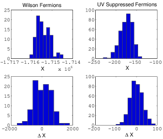
Figure 2. Upper panel: Distribution of the noisy estimator $X$ of the Wilson (left) and UV-sppressed (right) effective action. Lower panel: The same as in the upper panel but for the variation $\Delta X$ between two configurations. Lattice parameters: $12^{3}\times 24$, $\beta=5.9$, $m=-0.869$ ($\kappa=0.1597$), $\mu=0.2$.

The figure shows clearly that changes $\Delta X$ in the effective action estimator are reduced by an order of magnitude for UV-suppressed fermions as compared to Wilson fermions.

4. Concluding remarks

In this paper a lattice theory with suppressed cutoff modes of the fermion determinant is proposed. The level of suppression can be tuned by a new parameter $\mu$ that enters the theory. For $\mu\rightarrow\infty$ one recovers Wilson fermions whereas for $\mu\rightarrow 0$ one gets the quenched theory. For general $\mu$ the theory is similar to a Wilson theory with the effective cutoff $\sim\mu/a$.

By fixing $\mu$ at the appropriate value one can reduce considerably the UV fluctuations in the fermion determinant while preserving the interesting infrared modes of the theory. Thus one can eleminate the need to separate and then devise algorithms for the UV modes.

The fermion thoery described here can be easily extended to other input fermions such as staggered or chiral fermions.

Appendix A: Proof of the result (1.7)

I follow the analogous arguments as in Appendix C of [Hernández et al, 1999]. Using the definition of the Wilson operator (1.1), a straightforward computation yields:

$$\begin{array}[]{l}A(U)=D(U)_{W}^{{\dagger}}D(U)_{W}=\\ \\ +m^{2}\text{1\kern-2.41109ptl}-ma\sum_{\mu=1}^{4}\nabla_{\mu}\\ \\ +\sum_{\mu=1}^{4}(-\nabla_{\mu}^{2}+\frac{a^{2}}{4}\Delta_{\mu}^{2})+\sum_{\mu\neq\nu}\frac{a^{2}}{4}\Delta_{\mu}\Delta_{\nu}\\ \\ +\frac{1}{2}\sum_{\mu\neq\nu}\{-\gamma_{\mu}\gamma_{\nu}[\nabla_{\mu},\nabla_{\nu}]+a\gamma_{\mu}[\nabla_{\mu},\Delta_{\nu}]\}\end{array}$$

where

$$\begin{array}[]{l}4a^{2}[\nabla_{\mu},\nabla_{\nu}]\psi(x)=\\ \\ +[U(x)_{\mu}U(x+ae_{\mu})_{\nu}-U(x)_{\nu}U(x+ae_{\nu})_{\mu}]\psi(x+ae_{\mu}+ae_{\nu})\\ \\ +\text{3 similar terms}\end{array}$$

and

$$\begin{array}[]{l}2a^{3}[\nabla_{\mu},\Delta_{\nu}]\psi(x)=\\ \\ +[U(x)_{\mu}U(x+ae_{\mu})_{\nu}-U(x)_{\nu}U(x+ae_{\nu})_{\mu}]\psi(x+ae_{\mu}+ae_{\nu})\\ \\ +\text{3 similar terms}\end{array}$$

Note also that:

$$U(x)_{\mu}U(x+ae_{\mu})_{\nu}-U(x)_{\nu}U(x+ae_{\nu})_{\mu}=\text{1\kern-2.41109ptl}-U_{\mathbb{P}}$$

and

$$\left\|a^{2}[\nabla_{\mu},\nabla_{\nu}]\right\|_{2}=\left\|\text{1\kern-2.41109ptl}-U_{\mathbb{P}}\right\|_{2},~{}~{}~{}~{}~{}\left\|a^{2}[\nabla_{\mu},\Delta_{\nu}]\right\|_{2}=2\left\|\text{1\kern-2.41109ptl}-U_{\mathbb{P}}\right\|_{2}$$

Therefore, I obtain:

$$\left\|A(U)\right\|_{2}\leq\left\|D(\text{1\kern-2.41109ptl})_{W}\right\|_{2}^{2}+\frac{3}{2}\sum_{\mu\neq\nu}\left\|\text{1\kern-2.41109ptl}-U_{\mathbb{P}}\right\|_{2}$$

One can easily show that:

$$\left\|\text{1\kern-2.41109ptl}-U_{\mathbb{P}}\right\|_{2}\leq\left\|\text{1\kern-2.41109ptl}-U_{\mathbb{P}}\right\|_{F}=\sqrt{6[1-P(U)]}$$

where $\left\|.\right\|_{F}$ is the Frobenius (Euclidean) norm of a matrix. From the definition (1.5) and $\left\|D(\text{1\kern-2.41109ptl})_{W}\right\|_{2}\leq m+\frac{8}{a}$, $\left\|\delta A(U)\right\|_{2}\leq 2\left\|A(U)\right\|_{2}$ (assuming that $\left\|A(U+\delta U)\right\|_{2}\leq\left\|A(U)\right\|_{2}$), I obtain the result (1.7) with:

$$c_{1}=2(m+\frac{8}{a})^{2},~{}~{}~{}~{}~{}~{}c_{2}=36\sqrt{6}$$

Appendix B

To prove the statement I use similar algebraic manipulations to those used elsewhere in a different context [Boriçi, 1999a]. Here they appear in greater detail.

I let the lattice spacing in the fifth direction to be:

$$a_{5}=\frac{L_{5}}{n}$$

where $n$ is the number of lattice points in the fifth direction. The approximate fermion measure density can be defined by:

$$\omega_{n}(H_{W})=\frac{\det(\text{1\kern-2.41109ptl}-T^{n})}{\det(\text{1\kern-2.41109ptl}+T^{n})}$$

with $T$ being a classical transfer matrix:

$$T=\text{1\kern-2.41109ptl}-a_{5}H_{W}$$

It is easy to see that for small lattice spacing $a_{5}$, $\omega_{n}(H_{W})\rightarrow\omega(H_{W})$. It is only necessary to show that:

$$\det(D_{W}^{(5)})\sim\det(\text{1\kern-2.41109ptl}-{\tilde{T}}^{n})$$

where ${\tilde{T}}\rightarrow T$ as $a_{5}\rightarrow 0$. The right hand side can be realized for example as the determinant of the following $n\times n$ block matrix:

(4.1) $$\begin{pmatrix}\text{1\kern-2.41109ptl}&-{\tilde{T}}&&\\ &\text{1\kern-2.41109ptl}&\ddots&\\ &&\ddots&-{\tilde{T}}\\ -{\tilde{T}}&&&\text{1\kern-2.41109ptl}\\ \end{pmatrix}$$

where the sign of the left lower corner reverses if the boundary conditions of $D_{W}^{(5)}$ change from periodic to antiperiodic. Therefore, the ratio of the two determinants will be given by:

$$\frac{\det(\text{1\kern-2.41109ptl}-{\tilde{T}}^{n})}{\det(\text{1\kern-2.41109ptl}+{\tilde{T}}^{n})}\rightarrow\frac{\det(\text{1\kern-2.41109ptl}-T^{n})}{\det(\text{1\kern-2.41109ptl}+T^{n})}=\omega_{n}(H_{W})$$

One must now calculate ${\tilde{T}}$ from $D_{W}^{(5)}$. The fermion matrix can be written as an $n\times n$ block partition in the fifth dimension:

$$D_{W}^{(5)}=\begin{pmatrix}a_{5}D_{W}-\text{1\kern-2.41109ptl}&P_{+}&&P_{-}\\ P_{-}&a_{5}D_{W}-\text{1\kern-2.41109ptl}&\ddots&\\ &\ddots&\ddots&P_{+}\\ P_{+}&&P_{-}&a_{5}D_{W}-\text{1\kern-2.41109ptl}\\ \end{pmatrix}$$

where $P_{\pm}$ are the usual spin projector operators in the fifth direction. I multiply the above matrix from the left with the following permutation matrix:

$$\begin{pmatrix}P_{+}&P_{-}&&\\ &P_{+}&\ddots&\\ &&\ddots&P_{-}\\ P_{-}&&&P_{+}\\ \end{pmatrix}$$

and I obtain the following result:

$$\gamma_{5}\begin{pmatrix}a_{5}P_{+}H_{W}-\text{1\kern-2.41109ptl}&a_{5}P_{-}H_{W}+\text{1\kern-2.41109ptl}&&\\ &a_{5}P_{+}H_{W}-\text{1\kern-2.41109ptl}&\ddots&\\ &&\ddots&a_{5}P_{-}H_{W}+\text{1\kern-2.41109ptl}\\ a_{5}P_{-}H_{W}+\text{1\kern-2.41109ptl}&&&a_{5}P_{+}H_{W}-\text{1\kern-2.41109ptl}\\ \end{pmatrix}$$

Comparing this matrix to that containing ${\tilde{T}}$ (4.1) I arrive at the following expression for the transfer matrix:

$${\tilde{T}}=\frac{\text{1\kern-2.41109ptl}}{\text{1\kern-2.41109ptl}-a_{5}P_{+}H_{W}}(\text{1\kern-2.41109ptl}+a_{5}P_{-}H_{W})$$

which goes to $T^{-1}$ for small lattice spacing $a_{5}$. Since $T$ and $T^{-1}$ are equivalent transfer matrices the proof is concluded. ∎

Appendix C: Locality in the presence of gauge fields

To show locality of $D$ it is sufficient to show that the matrix-valued function $f(.)$ (3.3) is a local operator.

Let $p-$norm of the vector $v\in\mathbb{R}^{m},m\in\mathbb{N}$ be defined by:

$$\left\|v\right\|_{p}=(\sum_{k=1}^{m}|v_{k}|^{p})^{\frac{1}{p}}$$

with $p>0$. The induced matrix norm of $A\in\mathbb{R}^{m\times m}$ is defined by:

$$\left\|A\right\|_{p}=\max_{\left\|v\right\|_{p}=1}\left\|Av\right\|_{p}$$

If $x,y$ are two lattice points in four dimensions, I will refer to the matrix element $(x,y)$ of the matrix function $f$ as $f(x,y)$. Note that these elements are in fact matrices which carry spin and color indices, which I suppress for clarity.

I will show in the following that:

(4.2) $$\left\|f(x,y)\right\|_{2}\leq c_{1}c_{2}^{\frac{1}{a}\left\|x-y\right\|_{1}},~{}~{}~{}~{}~{}c_{1}>0,~{}~{}~{}~{}~{}0\leq c_{2}<1$$

for any $\mu>0$ and four dimensional lattice points $x,y$.

In order to prove (4.2) I need first to approximate the function $f$. From Appendix B one can infer that a five dimensional formulation gives a fermion measure density proportional to $\text{1\kern-2.41109ptl}-{\tilde{T}}^{n}$. Therefore one can write:

$$D\approx\frac{1}{a}\gamma_{5}\frac{\text{1\kern-2.41109ptl}-{\tilde{T}}^{n}}{\text{1\kern-2.41109ptl}+{\tilde{T}}^{n}}$$

This suggests the following approximation to the function $f$:

$$f(z^{2})\approx f_{n}(z^{2}):=\frac{1}{z}\frac{(1+\frac{z}{2n})^{2n}-(1-\frac{z}{2n})^{2n}}{(1+\frac{z}{2n})^{2n}+(1-\frac{z}{2n})^{2n}}$$

The right hand side can be expressed as a partial fraction by computing its poles and corresponding residues:

(4.3) $$f_{n}(z^{2})=\frac{1}{2n^{2}}\sum_{k=1}^{n}\frac{1}{(\frac{z}{2n})^{2}\cos^{2}\frac{\pi}{2n}(k-\frac{1}{2})+\sin^{2}\frac{\pi}{2n}(k-\frac{1}{2})}$$

Now I consider the matrix valued function $f_{n}$ with the matrix $\frac{aH_{W}}{\mu}$ substituted for the variable $z$ and show first that it is local for any approximation order $n$.

To simplify the notation, I call $A_{k}$ the matrix:

(4.4) $$A_{k}=(\frac{aH_{W}}{2n\mu})^{2}\cos^{2}\frac{\pi}{2n}(k-\frac{1}{2})+\sin^{2}\frac{\pi}{2n}(k-\frac{1}{2})$$

and write:

$$f_{n}[(\frac{aH_{W}}{\mu})^{2}]=\frac{1}{2n^{2}}\sum_{k=1}^{n}\frac{1}{A_{k}}$$

I use a geometric series to approximate the inverse of $A_{k}$ in order to keep the discussion simple (however note that a Chebyshev approximation is more accurate and is likely to decrease the exponent base $c_{2}$ of (4.2) in the final result [Hernández et al, 1999]). I may write:

(4.5) $$\frac{1}{A_{k}}=\frac{1}{\left\|A_{k}\right\|_{2}}\frac{1}{\text{1\kern-2.41109ptl}-(\text{1\kern-2.41109ptl}-\frac{A_{k}}{\left\|A_{k}\right\|_{2}})}$$

and then define:

$$\rho_{k}=\left\|\text{1\kern-2.41109ptl}-\frac{A_{k}}{\left\|A_{k}\right\|_{2}}\right\|_{2}$$

From the definition of the 2-norm I obtain:

$$\rho_{k}=1-\frac{1}{\left\|A_{k}\right\|_{2}\left\|A_{k}^{-1}\right\|_{2}}=1-\frac{1}{\kappa(A_{k})}$$

where $\kappa(A_{k})$ is the condition number of $A_{k}$. It is clear that $\rho_{k},k=1,\ldots,n$ are non-negative ($\kappa(A_{k})\geq 1$).

Let $\sigma_{1}\leq\sigma_{2}$ be the extreme singular values of $aD_{W}$. Then $\rho_{k}$ can be written as:

$$\rho_{k}=1-\frac{(\frac{\sigma_{1}}{2n\mu})^{2}\cos^{2}\frac{\pi}{2n}(k-\frac{1}{2})+\sin^{2}\frac{\pi}{2n}(k-\frac{1}{2})}{(\frac{\sigma_{2}}{2n\mu})^{2}\cos^{2}\frac{\pi}{2n}(k-\frac{1}{2})+\sin^{2}\frac{\pi}{2n}(k-\frac{1}{2})}$$

or

$$\rho_{k}=\frac{1-\frac{\sigma_{1}^{2}}{\sigma_{2}^{2}}}{1+(\frac{2n\mu}{\sigma_{2}})^{2}\tan^{2}\frac{\pi}{2n}(k-\frac{1}{2})}$$

But since $\tan z>z$ for $0<z<\frac{\pi}{2}$ (the range of $\tan$ argument values for $k=1,\ldots,n$) I obtain:

$$\rho_{k}<\frac{1-\frac{\sigma_{1}^{2}}{\sigma_{2}^{2}}}{1+\frac{[\mu\pi(k-\frac{1}{2})]^{2}}{\sigma_{2}^{2}}}$$

Clearly, I have:

(4.6) $$\rho_{k}<\rho_{1}<1,~{}~{}~{}~{}k=2,\ldots,n$$

Now I may expand the right hand side of (4.5) in geometric series to obtain:

$$\frac{1}{A_{k}}=\frac{1}{\left\|A_{k}\right\|_{2}}[\text{1\kern-2.41109ptl}+(\text{1\kern-2.41109ptl}-\frac{A_{k}}{\left\|A_{k}\right\|_{2}})+(\text{1\kern-2.41109ptl}-\frac{A_{k}}{\left\|A_{k}\right\|_{2}})^{2}+\cdots]$$

Further, I let the matrix $M_{k}$ to be:

$$M_{k}=(\text{1\kern-2.41109ptl}-\frac{A_{k}}{\left\|A_{k}\right\|_{2}})/\rho_{k}$$

such that the matrix elements of $f_{n}(.)$ can be given by:

$$f_{n}(x,y)=\frac{1}{2n^{2}}\sum_{k=1}^{n}\frac{1}{\left\|A_{k}\right\|_{2}}\sum_{l\geq 0}\rho_{k}^{l}M_{k}^{l}(x,y)$$

Since $A_{k}(x,y)$ vanishes for those lattice points $x,y$ such that $\left\|x-y\right\|_{1}>2a$, one may conclude that:

(4.7) $$M_{k}^{l}(x,y)=0,~{}~{}~{}~{}\text{for}~{}~{}~{}~{}\left\|x-y\right\|_{1}>2la,~{}~{}~{}~{}l=1,2,\ldots$$

In general I have:

(4.8) $$\left\|M_{k}^{l}(x,y)\right\|_{2}\leq 1,~{}~{}~{}~{}l=1,2,\ldots$$

Using (4.6), (4.7) and (4.8), I obtain:

$$\left\|f_{n}(x,y)\right\|_{2}<\rho_{1}^{\frac{1}{a}\left\|x-y\right\|_{1}}f_{n}[(\frac{\sigma_{2}}{\mu})^{2}]$$

But $zf_{n}(z^{2})\leq 1$ for $z>0$. Hence finally:

(4.9) $$\left\|f_{n}(x,y)\right\|_{2}<\frac{\mu}{\sigma_{2}}\rho_{1}^{\frac{1}{a}\left\|x-y\right\|_{1}}$$

Since the left hand side is uniformly bounded the result also holds in the limit $n\rightarrow\infty$. Hence the hypothesis (4.2) is proven with the constants $c_{1},c_{2}$ given by:

(4.10) $$c_{1}:=\frac{\mu}{\sigma_{2}},~{}~{}~{}~{}\text{and}~{}~{}~{}~{}c_{2}:=\frac{1-\frac{\sigma_{1}^{2}}{\sigma_{2}^{2}}}{1+\frac{\mu^{2}\pi^{2}}{4\sigma_{2}^{2}}}$$

∎

Remark. If the Wilson Dirac operator is singular (at $\sigma_{1}=0$, or at the “critical hopping parameter”) the locality of the theory is guaranteed solely by the positivity of $\mu$.

References

- [Bai et al, 1996] Z. Bai, M. Fahey, and G. H. Golub, Some large-scale matrix computation problems, J. Comp. Appl. Math., 74:71-89, 1996.
- [Boriçi, 1999a] A. Boriçi, Truncated Overlap Fermions: the link between Overlap and Domain Wall Fermions, in V. Mitrjushkin and G. Schierholz (edts.), Lattice Fermions and Structure of the Vacuum, Kluwer Academic Publishers, 2000.
- [Boriçi, 2002b] A. Boriçi, Computational Methods for UV-Suppressed Fermions, hep-lat/0208034.
- [Cahill et al, 1999] E. Cahill, A. Irving, C. Johnson, J. Sexton, Numerical stability of Lanczos methods, Nucl. Phys. Proc. Suppl. 83 (2000) 825-827
- [Duncan, Eichten and Thacker, 1999] A. Duncan, E. Eichten, H. Thacker, An Efficient Algorithm for QCD with Light Dynamical Quarks, Phys. Rev. D59 (1999) 014505
- [Edwards, Heller and Narayanan, 1998] R. G. Edwards, U. M. Heller, R. Narayanan, Spectral flow, condensate and topology in lattice QCD, Nucl. Phys. B535 (1998) 403-422.
- [de Forcrand, 1999] Ph. de Forcrand, UV-filtered fermionic Monte Carlo, Nucl. Phys. Proc. Suppl. 73 (1999) 822-824
- [Freund, 1993] R. W. Freund, Solution of Shifted Linear Systems by Quasi-Minimal Residual Iterations, in L. Reichel and A. Ruttan and R. S. Varga (edts), Numerical Linear Algebra, W. de Gruyter, 1993
- [Frommer et al, 1995] A. Frommer, S. Güsken, T. Lippert, B. Nöckel and K. Schilling, Many Masses on One Stroke: Economic Computation of Quark Propagators, Int. J. Mod. Phys. C6 (1995) 627-638 and hep-lat/9504020
- [Furman, Shamir, 1995] V. Furman, Y. Shamir, Axial symmetries in lattice QCD with Kaplan fermions, Nucl. Phys. B439 (1995) 54-78
- [Golub & Van Loan, 1989] G. H. Golub and C. F. Van Loan, Matrix Computations, The Johns Hopkins University Press, Baltimore, 1989
- [A. Hasenfratz & Knechtli, 2001] A. Hasenfratz and F. Knechtli, Simulating dynamical fermions with smeared links, Nucl. Phys. Proc. Suppl. 106 (2002) 1058-1060. See also A. Hasenfratz, Dynamical Simulation of Smeared Link Actions, Talk given at Lattice 2002, Boston, MA, USA.
- [Hernández et al, 1999] P. Hernandez, K. Jansen, and M. Lüscher, Locality properties of Neuberger’s lattice Dirac operator, Nucl. Phys. B552 (1999) 363
- [Irving et al, 1998] A. C. Irving, J. C. Sexton, E. Cahill, J. Garden, B. Joo, S. M. Pickles, Z. Sroczynsk , Tuning Actions and Observables in Lattice QCD, Phys. Rev. D58 (1998) 114504
- [Kikukawa, 2001] Y. Kikukawa, Analytic progress on exact lattice chiral symmetry, Nucl.Phys B (Proc.Suppl.) 106&107 (2002) 71-79
- [Lanczos, 1952] C. Lanczos, Solution of systems of linear equations by minimized iterations, J. Res. Nat. Bur. Stand., 49 (1952), pp. 33-53
- [Lüscher, 1998] M. Lüscher, Exact chiral symmetry on the lattice and the Ginsparg-Wilson relation, Phys. Lett. B428 (1998) 342-345
- [Peardon, 2001] M. Peardon, Progress in lattice algorithms Nucl. Phys. B (Proc.Suppl.) 106&107 (2002) 3-11. See also M. Peardon, Multiple molecular dynamics time-scales in Hybrid Monte Carlo fermion simulations, Talk given at Lattice 2002, Boston, MA, USA.
- [Wilson, 1974] K.G. Wilson, Confinement of quarks, Phys. Rev. D 10 (1974) pp. 2445-2459