BUTP/02/5, UCSD/PTH 02-04

Testing the fixed-point QCD action and the construction of chiral currents

P. Hasenfratz, S. Hauswirth, T. Jörg and F. Niedermayer

Institute for Theoretical Physics

University of Bern

Sidlerstrasse 5, CH-3012 Bern, Switzerland

K. Holland

Department of Physics

University of California at San Diego

9500 Gilman Drive, La Jolla CA 92093, USA

Abstract

We present the first set of quenched QCD measurements using the recently parametrized fixed-point Dirac operator $D^{\rm FP}$. We also give a general and practical construction of covariant densities and conserved currents for chiral lattice actions. The measurements include (a) hadron spectroscopy, (b) corrections of small chiral deviations, (c) the renormalized quark condensate from finite-size scaling and, independently, spectroscopy, (d) the topological susceptibility, (e) small eigenvalue distributions and random matrix theory, and (f) local chirality of near-zero modes and instanton-dominance.

1 Introduction

The only way to study a quantum field theory non-perturbatively from first principles is via lattice regularization. For a strongly-interacting theory like QCD, many essential features are non-perturbative. Over the course of more than two decades, lattice QCD has determined, with varying degrees of accuracy, the hadron mass spectra, quark masses, the strong interaction coupling constant, low-energy constants, inter-particle potentials, the phase structure of the theory, decay constants, matrix elements and many other quantities [1]. To make lattice QCD into a precise science requires detailed study of the systematic error introduced by the lattice discretization. As observed recently in a study of the $2d~{}O(3)$ non-linear sigma model [2], assumptions about how to extrapolate lattice results to the continuum may be wrong. Even for very accurate lattice measurements, large deviations as the lattice spacing $a$ is varied could mean large uncertainty in continuum quantities, due to the extrapolation ansatz. To reduce such sensitivity, many groups now use e.g. ${\cal O}(a)$-improved lattice actions to remove the leading order lattice artifacts. However, it may still be necessary to go to very fine resolution before the continuum extrapolation can be done confidently.

A separate issue is that, for a long time, it was thought impossible to have chiral lattice fermions [3]. This prevented a clean study of the chiral aspects of QCD, such as spontaneous symmetry breaking, and caused several technical headaches, such as fine-tuning the bare quark mass to make the pions light, exceptional configurations, mixing of operators with different chiral representations and additional renormalization factors. The question was also raised whether a chiral theory, such as the Standard Model, could in principle be defined non-perturbatively. The domain wall fermions [4], the related overlap construction [5] and the fixed-point (FP) action [6] are the known examples for lattice regularized fermions with chiral symmetry. The common feature behind these rather different constructions is the Ginsparg-Wilson (GW) relation [7] which is satisfied by all these constructions [8]. Actually, one might construct a Dirac operator using directly the GW relation and the requirement of locality [9]. The GW relation not only implies all the physical consequences of chiral symmetry [10, 11], but also the existence of an exact symmetry transformation [12]. This has caused an explosion of interest in the last few years in theory [13] and in using different methods to explore the chiral behavior of quenched QCD (no sea quarks), which is now quickly maturing. With the standardly used algorithms, it is impossible to use chiral lattice actions for simulations of full QCD (with sea quarks), as these actions have a complicated structure [14]. This is the major obstacle for the future use of chiral actions. For a recent promising development see, however, ref. [15].

The fixed-point method is motivated by renormalization group properties of lattice field theories [16]. Instead of trying to remove lattice artifacts order by order in the lattice spacing $a$, a fixed-point (FP) action is designed to be less sensitive to the discretization even at large lattice spacings. In fact, for some quantities, a FP action is entirely blind to the discretization. An exact FP QCD action has exact chiral symmetry and offers a completely new approach to examine the chiral properties of the theory. Exact and approximate fixed-point actions have been constructed and tested for a number of models, including pure Yang-Mills theory, and in general have shown very good scaling behavior [17, 18]. The construction and initial tests of an approximate fixed-point Dirac operator $D^{\rm FP}$ are described in [20]. Like other chiral actions, fixed-point actions are more costly to use in simulations than standard actions. However, FP actions are designed to have much reduced lattice artifacts and, if chiral actions are the correct long-term approach for lattice QCD, FP actions might be the optimal choice.

In this paper, we present the results of a preliminary study of an approximate FP QCD action, to test if it is feasible to use such an action in simulations. A larger systematic study, which is running already as part of the program of the Bern-Graz-Regensburg Collaboration, is required to examine the lattice spacing dependence of measurements using this action (see ref. [19]). As well as these initial measurements, we also give a practical method to construct and use conserved currents in simulations with chiral lattice actions. Many groups now use chiral actions, but non-conserved currents and/or non-covariant densities and so lose part of the advantages offered by a chiral formulation.

This paper is a detailed description of the work summarized in [21, 22]. The paper is organised as follows. In Section 2, we examine how small chiral deviations of the action can be corrected. Hadron spectroscopy measurements with the parametrized FP Dirac operator are described in Section 3, giving the pion, rho and nucleon masses, the speed of light, the remnant additive quark mass renormalization and an indication of the presence of quenched chiral logarithms. In Section 4, we use the overlap-improved FP Dirac operator to measure the meson spectrum, the renormalized quark condensate via finite-size scaling, the quenched topological susceptibility, investigate random matrix theory and small eigenvalue distributions on small lattice volumes, and examine instanton-dominance of near-zero modes of the Dirac operator. The construction of covariant currents and densities and a discussion of Ward identities for chiral lattice actions are given in Section 5, followed by our conclusions. In the Appendix we collect some useful identities which are implied by the Ginsparg-Wilson relation.

2 Chiral behavior of ${\mathbf{D}^{\rm FP}}$

A Dirac operator $D$ which satisfies exactly the Ginsparg-Wilson relation

$${\gamma_{5}}D+D{\gamma_{5}}=D{\gamma_{5}}2RD\,,$$ (1)

where $R$ is any local function and trivial in Dirac space, has exact chiral symmetry even at non-zero lattice spacing $a$. Such a Dirac operator has infinitely many couplings [23]. Simulations are only feasible with a finite number of couplings, hence the chiral symmetry is only approximate. What needs to be examined is how good the approximation is. The exact fixed-point Dirac operator satisfies exactly the Ginsparg-Wilson relation. The parametrized fixed-point Dirac operator $D^{\rm FP}$, which we use in simulations, is an approximate solution to the QCD fixed-point equations. The construction and initial tests of $D^{\rm FP}$ are described in [21, 22]. Here, we test the quality of the chiral symmetry of this operator.

As will be discussed in Sec. 5, the function $2R$ can be absorbed into the definition of $D$, so for simplicity, we set $2R=1$ in most of the following equations. The Ginsparg-Wilson relation can be re-written as

$$D+D^{\dagger}=D^{\dagger}D,$$ (2)

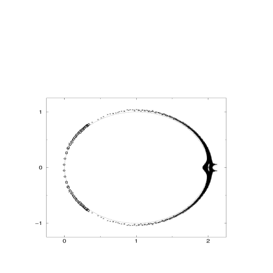
Figure 1: The full eigenvalue spectrum of $D^{\rm FP}$ for a $S^{\rm FP}_{g}$ gauge configuration of volume $4^{4}$ (crosses) and the smallest 100 eigenvalues on a $8^{4}$ volume (circles) at a lattice spacing $0.16\,{\rm fm}$.

using the property ${\gamma_{5}}D{\gamma_{5}}=D^{\dagger}$. If $D$ satisfies this relation, its complex eigenvalues lie on the circle of radius 1 and centre at (1,0) in the complex plane. In Fig. 1, we plot the complex eigenvalues of $D^{\rm FP}$ for fixed-point gauge action $S^{\rm FP}_{g}$ configurations. The lattice spacing can be determined via the Sommer parameter $r_{0}$ of the static quark anti-quark potential. To orient the reader, the bare coupling of the gauge action $\beta=6/g^{2}=3.0$ and $3.2$ correspond to lattice spacings $a\simeq 0.16\,{\rm fm}$ and $a\simeq 0.13\,{\rm fm}$, respectively. The figure contains all the eigenvalues for $4^{4}$ gauge configurations and those closest to the origin for $8^{4}$ configurations. It’s clear that the breaking of the Ginsparg-Wilson relation is small over the entire eigenvalue spectrum even though the lattice spacing is quite coarse, and that the chiral symmetry remains very good even for larger volumes. For comparison, the eigenvalues of the Wilson Dirac operator $D^{\rm W}$ at a similar lattice spacing are very far removed from the Ginsparg-Wilson circle [24].

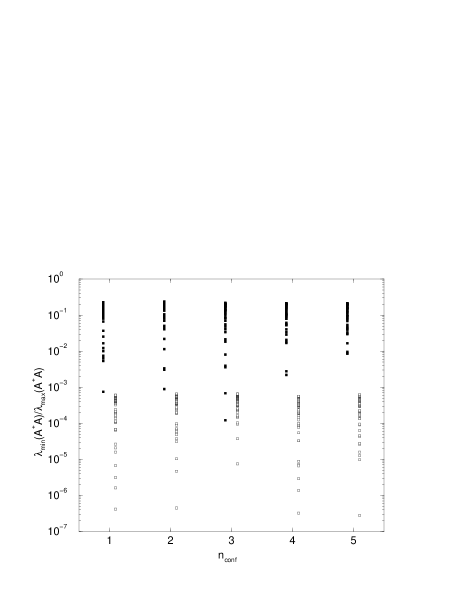
Figure 2: Ratio of the 50 smallest $A^{\dagger}A$ eigenvalues to the largest eigenvalue using $D^{\rm FP}$ (filled squares) and $D^{\rm Wilson}$ (open squares) for 5 different $S^{\rm FP}_{g}$ gauge configurations of volume $12^{4}$ at a lattice spacing $0.16\,{\rm fm}$.

Defining the operator $A=1-D$, the Ginsparg-Wilson relation is equivalent to the requirement that $A$ be unitary i.e. $A^{\dagger}A=1$. We can measure how much this requirement is broken by finding the smallest and largest eigenvalues of $A^{\dagger}A$. In Fig. 2, we plot the ratio of the 50 smallest eigenvalues of $A^{\dagger}A$ to the largest eigenvalue for a number of $S^{\rm FP}_{g}$ gauge configurations with a lattice spacing $0.16\,{\rm fm}$. The largest eigenvalue is approximately 1.5 and 38 for $D^{\rm FP}$ and $D^{\rm W}$ respectively. We see that the fixed-point operator is much closer than the Wilson operator to satisfying the unitarity condition. Also, as the volume increases, it’s more likely that using $D^{\rm FP}$ produces a few very small eigenvalues, but the vast bulk of the $A^{\dagger}A$ spectrum is close to 1.

For some measurements, it’s necessary that the remnant chiral symmetry breaking be very small. Given any suitable Dirac operator $D_{0}$ as input, the overlap Dirac operator [5]

$$D_{\rm ov}=1-A/\sqrt{A^{\dagger}A},\hskip 28.45274ptA=1+s-D_{0}$$ (3)

is an exact solution of the Ginsparg-Wilson relation. The real parameter $s$ can be used to optimize the convergence of approximations or the locality of the resulting overlap Dirac operator. The nice feature of this operator is that it’s an explicit construction, unlike the fixed-point operator which is a solution to a set of equations. If the input operator $D_{0}$ is already chiral, then $A^{\dagger}A=1$ and hence $D_{\rm ov}=D_{0}$. Most simulations using $D_{\rm ov}$ have taken $D^{\rm W}$ as the input operator, which has severely broken chiral symmetry, as $A^{\dagger}A$ is far from 1 and hence computing $1/\sqrt{A^{\dagger}A}$ is a very expensive numerical problem. A measure of this difficulty is the condition number of $A^{\dagger}A$, the ratio of its smallest to largest eigenvalue. Also, the overlap operator may inherit the large lattice artifacts of $D^{\rm W}$. Alternatively, taking $D^{\rm FP}$ as the input operator, $A^{\dagger}A$ is close to 1 and $1/\sqrt{A^{\dagger}A}$ is easier to evaluate — the improvement in the condition number is clear in Fig. 2. The overlap construction should only bring small corrections to $D^{\rm FP}$. This way, the residual chiral symmetry breaking can be removed without destroying the very important fixed-point properties.

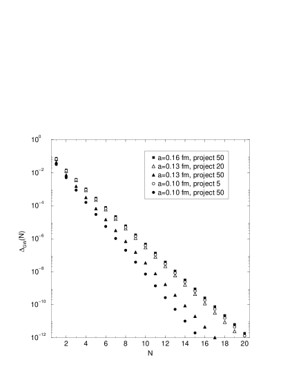
Figure 3: Breaking of the Ginsparg-Wilson relation as measured by $\Delta_{\rm GW}(N)$ on $10^{4}$ lattices at different lattice spacings and different number of exactly projected $A^{\dagger}A$ eigenvalues. Keeping the number of exactly projected $A^{\dagger}A$ eigenvalues constant, the exponential fall-off is steeper for smaller lattice spacings. If the number of exactly projected $A^{\dagger}A$ eigenvalues is adjusted such that the range of the not exactly treated $A^{\dagger}A$ eigenvalues is approximately the same for the different lattice spacings, the fall-off is roughly equal in all cases, which illustrates that the approximation is governed by the ratio $\lambda_{\rm min}(A^{\dagger}A)/\lambda_{\rm max}(A^{\dagger}A)$.

As the chiral symmetry is already well approximated by $D^{\rm FP}$, we use a Legendre polynomial approximation of $1/\sqrt{A^{\dagger}A}$ to construct the overlap-improved operator $D_{\rm ov}^{\rm FP}$. As $A^{\dagger}A$ may occasionally have a few very small eigenvalues, we always project out the smallest 10 to 100 eigenvalues, which are treated exactly. One measure of the remnant chiral symmetry breaking is the vector norm $\Delta_{\rm GW}=||(D+D^{\dagger}-D^{\dagger}D)v||$, where $v$ is a unit vector of random entries. If $D$ solves the Ginsparg-Wilson relation, $\Delta_{\rm GW}$ vanishes. In Fig. 3, we plot $\Delta_{\rm GW}(N)$ versus the order $N$ of the polynomial used to approximate $1/\sqrt{A^{\dagger}A}$ for gauge configurations of volume $10^{4}$ at different lattice spacings ($0.16\,{\rm fm}$, $0.13\,{\rm fm}$, $0.10\,{\rm fm}$). The chiral symmetry breaking falls off exponentially as the polynomial order increases. The rate of the fall off varies depending on the range of the $A^{\dagger}A$ eigenvalues which are not projected out. Projecting out the same number of $A^{\dagger}A$ eigenvalues for the different lattice spacings, the rate of the fall off is the largest for the smallest lattice spacing. However, choosing the number of projected $A^{\dagger}A$ eigenvalues such that ratio $\lambda_{\rm min}(A^{\dagger}A)/\lambda_{\rm max}(A^{\dagger}A)$ for the remaining $A^{\dagger}A$ eigenvalues is approximately the same for the three different lattice spacings, the rate of the fall off is roughly equal for all the lattice spacings, which illustrates that the convergence rate is indeed governed by the ratio $\lambda_{\rm min}(A^{\dagger}A)/\lambda_{\rm max}(A^{\dagger}A)$.

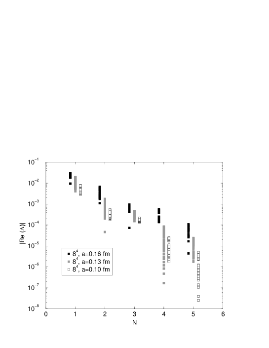
Figure 4: The dependence of the deviation of the $D_{\rm ov}^{\rm FP}$ eigenvalues from the Ginsparg-Wilson circle on the order of the polynomial approximation, as measured by $|{\rm Re}(\Lambda)|$.

If the eigenvalues $\lambda_{n}$ of $D$ lie exactly on the Ginsparg-Wilson circle, then $\Lambda_{n}=\lambda_{n}/(1-\lambda_{n}/2)$ are purely imaginary i.e. the eigenvalues are projected from the circle onto the imaginary axis. In Fig. 4, we plot $|{\rm Re}(\Lambda_{n})|$ versus the order of polynomial used to approximate $1/\sqrt{A^{\dagger}A}$, for gauge configurations with lattice spacings $0.16,0.13$ and $0.10\,{\rm fm}$. As the order increases, $|{\rm Re}(\Lambda_{n})|$ becomes exponentially small as the eigenvalues $\lambda_{n}$ lie closer and closer to the Ginsparg-Wilson circle, with the most rapid decrease at the finest lattice spacing.

A lattice action must be local for its continuum predictions to be universal i.e. independent of the choice of lattice discretization. Locality on the lattice means that fields at large separation have an exponentially small coupling. The exponential decay of the action should be faster than that of the correlation functions. This issue was first addressed for the overlap operator $D_{\rm ov}$ in [25], where a free parameter was varied to maximize the exponential fall-off. One measure of locality is

$$f(r)=\max_{y}\{||D_{\rm ov}v||,||y-x||=r\},$$ (4)

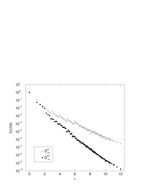
Figure 5: The locality of $D_{\rm ov}$, as measured by the expectation value $f(r)/f(0)$ defined in Eq. (4), using $D^{\rm FP}$ and $D^{\rm Wilson}$ as input on $12^{4}$ lattices at $a=0.16\,{\rm fm}$.

where $v$ is vector with a point source at $x$ and $r$ is the square norm. In Fig. 5, we plot the expectation value of $f(r)/f(0)$ versus $r$ for different overlap operators on $12^{4}$ volumes at a lattice spacing of $0.16\,{\rm fm}$. Compared with other tests of locality of $D_{\rm ov}$ using $D^{\rm W}$ as input [25, 26], the locality is significantly improved if the overlap operator is constructed using $D^{\rm FP}$, with a faster exponential decay. The exponent $\nu$ describing the decay at large separation $r$ is $\nu=0.94$ for $D^{\rm W}_{\rm ov}$, whereas it is $\nu=1.60$ for $D^{\rm FP}_{\rm ov}$. In order to optimize the locality of $D^{\rm W}_{\rm ov}$ the parameter $s$ in Eq. (3) has to be tuned and we find $s=0.6$ as optimal value at this lattice spacing. In contrast to $D^{\rm W}_{\rm ov}$ there is no tuning of the parameter $s$ needed for $D^{\rm FP}_{\rm ov}$ to get the (approximately) optimal locality, i.e.we can use $s=0.0$ for $D^{\rm FP}_{\rm ov}$.

From these tests, we see that the chiral symmetry is well approximated by $D^{\rm FP}$ and that the residual breaking can be removed using overlap-improvement. Only a relatively low order polynomial approximation is required to construct $D_{\rm ov}^{\rm FP}$, which is essential as $D^{\rm FP}$ is more expensive to use than $D^{\rm W}$. The parametrized FP operator has 9 times more offsets and the computational cost per offset is also higher since $D^{\rm FP}$ includes all elements of the Clifford algebra. If, in a matrix-vector multiplication, for $D^{\rm W}$ the time needed for Dirac matrix multiplications is neglected, then $D^{\rm FP}$ is a factor of $\approx 4$/offset more expensive leading to an estimated relative overhead of $\approx 36$. Note, however, that this number may vary quite a bit depending on the underlying computer architecture, as one of the main issues in present lattice simulations is rather fast memory access and fast communication than fast floating point units [27].

3 Spectroscopy

Measuring the mass spectrum is a standard benchmark for using a particular lattice action. Simulations with improved Wilson and staggered fermions in full QCD are now very advanced in reaching the physical theory. Mass spectroscopy in quenched QCD with chiral fermions is quickly maturing and is a very good test of the chiral behavior of the theory. In this preliminary study, we test the behavior of $D^{\rm FP}$, for example, how intact are the fixed-point properties, how large is the additive quark mass renormalization, how small an $m_{\pi}/m_{\rho}$ ratio can be attained and do we observe quenched chiral logarithms.

3.1 Simulation parameters

The FP gauge action we use has previously been studied in detail [17]. To remind the reader, the bare coupling of the gauge action $\beta=6/g^{2}=3.0$ and $3.2$ correspond to lattice spacings $a\simeq 0.16\,{\rm fm}$ and $a\simeq 0.13\,{\rm fm}$ respectively, as determined from the Sommer parameter $r_{0}$ of the static quark anti-quark potential [28]. Lattice volumes of $6^{3}\times 16$ and $9^{3}\times 24$ are compared to investigate the volume dependence of zero mode effects. We use gaussian smeared sources and point sinks. Configurations were fixed to Landau gauge using the Los Alamos algorithm with stochastic overrelaxation [29]. With the parametrized FP Dirac operator $D^{\rm FP}$, we simulate at input quark masses $ma$ ranging from 0.016 to 0.23. The smallest quark mass corresponds to $m_{\pi}/m_{\rho}=0.30(3)$. It has to be stressed that we introduce the mass in the most simple manner by defining $D(m)=D^{\rm FP}+m$ or with the covariant scalar density in Eq. (88) $D(m)=(1-m/2)D^{\rm FP}+m(2R)^{-1}$, whereas the fixed-point Dirac operator for non-zero mass would in fact need a reparametrization by iteratively solving the RG transformations for every mass value as we did for the zero-mass Dirac operator $D^{\rm FP}$. Therefore our parametrization deviates more and more from the classical renormalized trajectory for larger masses. A multimass BiCGstab algorithm [30] is used to invert the Dirac operator at all masses simultaneously. Errors are estimated with bootstrap resampling of the hadron correlators, which were symmetrized around $t=T/2$ to increase statistics. A correlated fit to the measured correlators is performed in the interval $[t_{\rm min},t_{\rm max}]$, where the minimum time $t_{\rm min}$ of the fit range is determined by two criteria: i) the effective mass starts to show a reasonable plateau, ii) the value of $\chi^{2}$ per degree of freedom in the fit ($\chi^{2}/df$) starts to show a plateau and is of order 1. The maximum time $t_{\rm max}$ is generally set to $T/2$ in the mass measurements, while for the finite momentum measurements it is reduced according to the length of the plateau.

fermion action	lattice size	$\beta$	$L_{s}$	$N_{\rm conf}$	$ma$
parametrized FP	$6^{3}\times 16$	3.0	1.0 fm	96	$0.02,\dots,0.20$
parametrized FP	$9^{3}\times 24$	3.0	1.5 fm	70	$0.016,\dots,0.23$
overlap FP	$9^{3}\times 24$	3.0	1.5 fm	28	$0.012,\dots,0.23$
overlap FP	$9^{3}\times 24$	3.2	1.2 fm	32	$0.012,\dots,0.23$

Table 1: Simulation parameters for hadron spectroscopy.

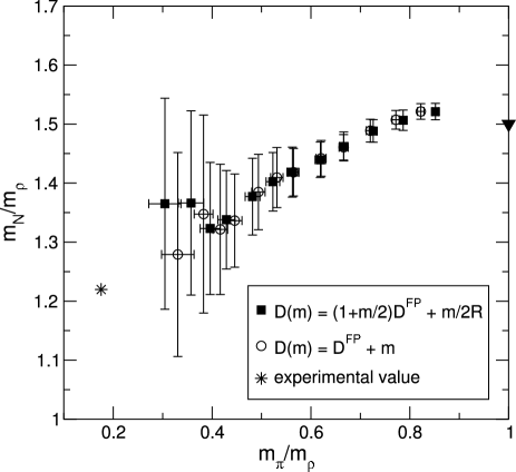
Figure 7: Edinburgh plot for the parametrized FP Dirac operator on $9^{3}\times 24$ at $\beta=3.0$ for the naive and covariant mass definition.

Fig. 6 shows the masses of the pseudoscalar and vector meson and the nucleon measured with the parametrized FP Dirac operator on the $9^{3}\times 24$ lattice. The inversion of the Dirac operator converged for all configurations within reasonable time, although for one configuration the number of inversions was about three times larger than the typical value of $\approx 250$. This indicates that the residual chiral symmetry breaking leads to fluctuations on the order of our smallest quark mass for the real eigenvalues of the Dirac operator, and therefore it would not be wise to go to smaller masses than $ma=0.016$ with the parametrized FP operator at this lattice spacing and volume. An extrapolation of the rho mass to the physical value gives a lattice spacing of $a\simeq 0.17\,{\rm fm}$, which is slightly higher than that obtained from the Sommer parameter. The sign and size of this deviation is consistent with earlier findings [31]. Fig. 7 is an Edinburgh plot from this data.

3.2 The pion mass in the chiral limit

A lattice calculation of the pion mass in the limit of small quark mass with the FP action is interesting for several reasons: first, it serves as a quantitative check of how chiral our action actually is. For an exactly chiral fermion action like the overlap or the exact fixed-point action, there is no additive renormalization of the quark mass. But does the approximation we make by parametrizing the FP action introduce a residual mass, and can we measure it? Second, at the lattice volumes we are working with, one expects to see topological finite-volume effects proportional to $1/(m_{q}^{2}\sqrt{V})$ and $1/(m_{q}\sqrt{V})$ [32] which complicate a reliable pion mass measurement at small quark masses. It is therefore crucial to check whether these effects are under control. Third, having an action with good chiral properties at hand, one can check for the appearance of logarithmic terms in the chiral extrapolation of the squared pion mass.

$ma$	$m_{\pi}$(P)	$\chi^{2}/df$	$m_{\pi}$(A)	$\chi^{2}/df$	$m_{\pi}$(P-S)	$\chi^{2}/df$
0.02	0.394(41)	0.77	0.345(62)	1.55	0.273(33)	1.19
0.03	0.398(25)	1.01	0.381(30)	0.62	0.341(32)	0.72
0.04	0.416(19)	0.92	0.403(21)	0.64	0.381(28)	0.47
0.05	0.439(16)	0.87	0.428(19)	0.80	0.418(22)	0.33
0.06	0.463(14)	0.90	0.451(17)	0.98	0.451(21)	0.25
0.08	0.502(15)	0.91	0.498(14)	1.14	0.512(18)	0.19
0.10	0.546(13)	0.74	0.541(12)	1.10	0.566(16)	0.22
0.13	0.611(12)	0.53	0.603(10)	0.93	0.638(16)	0.37
0.16	0.672(11)	0.38	0.663(10)	0.78	0.703(15)	0.64
0.20	0.748(10)	0.26	0.737(08)	0.64	0.783(13)	1.11

Table 2: Pion masses for parametrized FP fermions on $6^{3}\times 16$ lattice from three different pion operators. The quark mass is introduced by $D^{\rm FP}(m)=D^{\rm FP}+m$.

We use three different operators to extract the pion mass: the pseudoscalar $P=\overline{\Psi}{\gamma_{5}}\Psi$, the fourth component of the axial vector $A_{4}=\overline{\Psi}\gamma_{4}{\gamma_{5}}\Psi$ and the difference of pseudoscalar and scalar $S=\overline{\Psi}\Psi$. In the quenched theory, the pseudoscalar correlator $\langle P(x)P(0)\rangle$ is contaminated by the topological finite size effects from configurations with non-trivial topology, as mentioned above. The same special finite size contributions appear in the scalar correlator, so by building the difference of the pseudoscalar and scalar correlator $\langle P(x)P(0)\rangle-\langle S(x)S(0)\rangle$, this artificial effect should cancel, although if the action is not exactly chiral, the cancellation is also not exact. For larger quark masses, the P-S correlator is contaminated by effects from the scalar part and is expected to deviate from the pion. For the axial vector correlator $\langle A_{4}(x)A_{4}(0)\rangle$, the divergent contribution is expected to be partially suppressed [32, 33].

$ma$	$m_{\pi}$(P)	$\chi^{2}/df$	$m_{\pi}$(A)	$\chi^{2}/df$	$m_{\pi}$(P-S)	$\chi^{2}/df$
0.016	0.267(20)	1.25	0.223(15)	0.53	0.209(21)	0.64
0.02	0.274(15)	1.18	0.256(14)	0.72	0.243(16)	0.66
0.025	0.292(11)	0.92	0.281(10)	0.68	0.272(13)	0.72
0.03	0.314(8)	0.93	0.306(9)	0.88	0.298(11)	0.80
0.04	0.351(7)	0.98	0.346(8)	1.12	0.342(9)	0.89
0.05	0.384(6)	1.06	0.381(7)	1.23	0.379(8)	0.97
0.06	0.415(6)	1.13	0.413(7)	1.25	0.413(7)	1.06
0.08	0.473(6)	1.27	0.473(6)	1.20	0.476(6)	1.24
0.10	0.526(5)	1.38	0.526(6)	1.16	0.532(5)	1.41
0.13	0.601(4)	1.52	0.600(5)	1.16	0.609(5)	1.69
0.17	0.692(4)	1.71	0.691(5)	1.30	0.703(4)	2.00
0.23	0.819(3)	2.00	0.817(4)	1.76	0.832(4)	2.16

Table 3: Pion masses for parametrized FP fermions on $9^{3}\times 24$ lattice from three different pion operators.

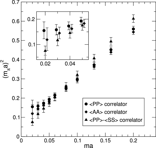
Figure 8: Squared pion mass for the parametrized FP Dirac operator $D^{\rm FP}$ from 100 $6^{3}\times 16$ gauge configurations. The inset shows the smallest four masses on a magnified scale to identify topological finite-volume effects.

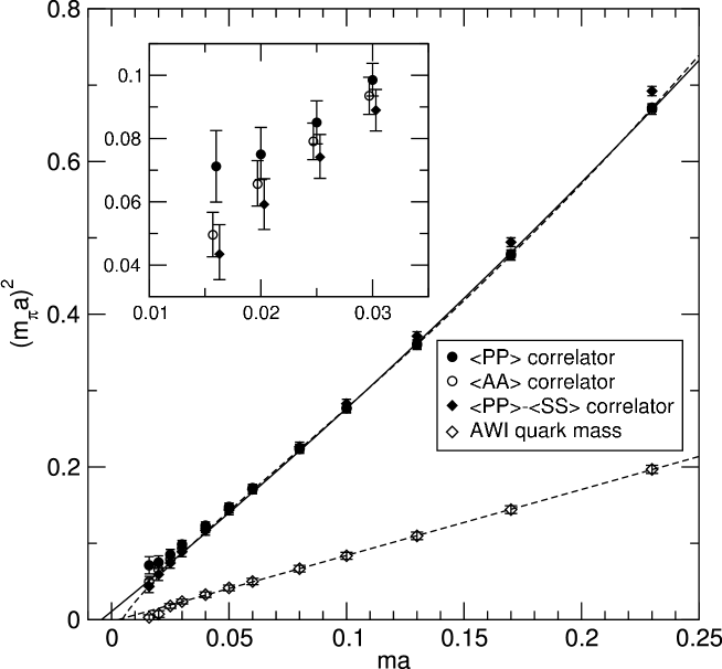
Figure 9: Squared pion mass for the parametrized FP Dirac operator $D^{\rm FP}$ from 70 $9^{3}\times 24$ gauge configurations. The massive Dirac operator is constructed with the covariant scalar density as in Eq. (88). Shown are quadratic fits to the P correlator at large and the P-S correlator at small quark mass with (dashed line) and without (solid line) the Q$\chi$PT logarithm. The inset shows the smallest four masses on a magnified scale. Topological finite-volume effects are reduced considerably. Also plotted is the unrenormalized quark mass from the axial Ward identity (AWI) together with a linear fit. When the quenched chiral logarithm is included in the fit, the fits from the AWI quark mass and from the squared pion mass agree in the chiral limit.

Figs. 8 and 9 show a comparison of the squared pion mass versus the input quark mass at the two lattice sizes $6^{3}\times 16$ and $9^{3}\times 24$ using the parametrized FP Dirac operator. On the smaller volume, the three different pion correlators give very different values at small quark masses. The P correlator lies highest, while the P-S correlator gives considerably smaller pion masses, as the inset in Fig. 8 shows. The A correlator lies in between the two. This behaviour is in qualitative agreement with the results from domain-wall fermions [32]. For larger quark masses, the P-S correlator deviates from the other two, as it is then difficult to disentangle the contribution of the closely lying scalar state in the mass determination, which can also be seen from the increasing value of $\chi^{2}$ for the mass fit in Table 3. As expected, the discrepancy between the three correlators in the chiral limit is reduced at our larger lattice volume. The ordering among the correlators is still the same, but the pion mass difference is smaller. A recent study with Wilson overlap fermions at a similar spatial lattice size of $\approx 1.4\,{\rm fm}$ also shows no significant difference [36], but their smallest quark mass is much larger than ours. We can conclude from our findings that at the rather small statistics that we have collected, the topological finite-volume effects become non-negligible at the smallest few quark masses, where the pseudoscalar correlator is clearly contaminated and cannot be used to get reliable results. We therefore decide to work in the following with the P-S correlator at small and with the P correlator at large quark mass, changing correlators at an intermediate quark mass where both agree, which is at $ma=0.06$ for the $9^{3}\times 24$ lattice.

$ma$	$m_{\pi}/m_{\rho}$	$m_{\rho}$	$\chi^{2}/df$	$m_{N}$	$\chi^{2}/df$
0.016	0.304(33)	0.673(21)	0.87	0.919(117)	0.66
0.02	0.357(26)	0.679(21)	0.48	0.928(102)	0.83
0.025	0.396(20)	0.686(14)	1.06	0.908(74)	0.95
0.03	0.429(17)	0.693(12)	1.42	0.927(55)	1.03
0.04	0.482(15)	0.708(12)	1.79	0.975(43)	1.43
0.05	0.523(14)	0.723(11)	2.02	1.013(32)	1.82
0.06	0.562(11)	0.735(10)	2.20	1.043(27)	2.38
0.08	0.619(10)	0.763(9)	2.45	1.098(19)	2.97
0.10	0.666(9)	0.788(9)	2.56	1.152(15)	3.22
0.13	0.726(8)	0.828(7)	2.51	1.232(11)	3.46
0.17	0.786(7)	0.886(7)	2.28	1.335(11)	3.71
0.23	0.852(6)	0.979(6)	2.16	1.489(10)	4.17

Table 4: $m_{\pi}/m_{\rho}$, rho and nucleon masses for parametrized FP fermions on $9^{3}\times 24$ lattice.

On the larger lattice, we also measure the unnormalized AWI quark mass

$$2m_{q}(t)=\frac{\sum_{\vec{x}}\langle\partial_{4}A_{4}(\vec{x},t)P(0)\rangle}{\sum_{\vec{x}}\langle P(\vec{x},t)P(0)\rangle},$$ (5)

and take the average of the ratio of correlators over the range $5\leq t\leq 9$. We use an ultralocal (non-conserved) axial current $A_{\mu}$ and neglect the renormalization factors $Z_{A}$ and $Z_{P}$ which would show up on the right hand side of Eq. (5), as they are not relevant for the following analysis. We fit the data with a linear function to determine whether the remaining chiral symmetry breaking of the action introduces a residual mass. The smallest two masses were left out of the fit, which is shown as a dashed line in Fig. 9. From the intersection of the linear fit with the horizontal axis we read off a residual mass $m_{\rm res}^{\rm AWI}a=-0.003(4)$, which is consistent with zero within errors. A quadratic fit to the squared pion mass from the P-S correlator for $am\leq 0.05$ and the P correlator for $am>0.05$ gives $m_{\rm res}a=0.004(4)$ with a value of $\chi^{2}/df=0.28$, while a fit to the form predicted by quenched chiral perturbation theory (Q$\chi$PT) [39]

$$m_{\rm PS}^{2}=2A(m_{q}+m_{\rm res})\left[1-\delta\left(\ln\frac{2A(m_{q}+m_{\rm res})}{\Lambda_{\chi}^{2}}+1\right)\right]+4B(m_{q}+m_{\rm res})^{2},$$ (6)

gives $m_{\rm res}a=-0.004(5)$ and $0.23(7)<\delta<0.30(18)$ when the scale $\Lambda_{\chi}$ is varied in the range between $0.8\,{\rm GeV}$ and $1.2\,{\rm GeV}$, with typical values of $\chi^{2}/df=0.05$. Obviously the large errors do not allow to single out a preferred form for the chiral fit, but for the Q$\chi$PT form, the residual quark mass agrees with the one from the axial Ward identity, while the agreement is worse in the case of the quadratic fit. This gives a hint that we see a signal of the chiral logarithm in our pion mass measurements. (Note that the smallness of the $\chi^{2}/df$ values is due to the fact that the results for different quark masses are strongly correlated, hence an improvement from $0.28$ down to $0.05$ is meaningful.)

3.3 Energy-momentum dispersion relation

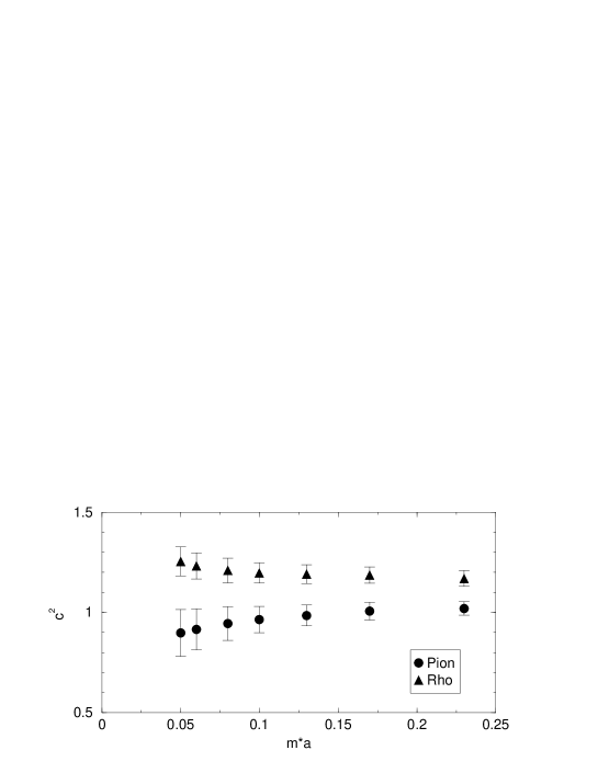
Figure 10: Squared speed of light $c^{2}$ for pion and rho mesons with the parametrized FP Dirac operator $D^{\rm FP}+m$ at the smallest non-zero momentum. The error bars are from statistical errors only. Systematic uncertainties from choosing the fit range (especially for the rho) would increase the errors considerably.

As the FP action is classically perfect, its dispersion relation is expected to show small scaling violations. In Fig. 10 the squared speed of light $c^{2}=(E(p)^{2}-m^{2})/p^{2}$ measured on the $9^{3}\times 24$ lattice is shown for the smallest momentum $\vec{p}=2\pi\vec{n}/9$ with $|\vec{n}|=1$ ($|\vec{p}|\approx 0.8\,{\rm GeV}$) at different quark masses. While $c^{2}$ for the pion is consistent with 1 within errors, it is not for the rho meson. However, the (purely statistical) error bars do not include systematic uncertainties from choosing the fit range, which was especially difficult for the rho in this low statistics, small volume study. As a qualitative result, it is clear that compared to the Wilson or Sheikholeslami-Wohlert clover action [37], the dispersion relation is significantly improved.

$ma$	$m_{\pi}/m_{\rho}$	$m_{\pi}$(P)	$m_{\pi}$(A)	$m_{\pi}$(P-S)	$m_{\rho}$
0.012	0.273(38)	0.235(12)	0.232(15)	0.202(23)	0.741(56)
0.016	0.313(32)	0.257(19)	0.258(13)	0.234(20)	0.747(43)
0.02	0.348(29)	0.279(10)	0.280(12)	0.261(18)	0.752(36)
0.03	0.418(24)	0.326(8)	0.328(11)	0.319(14)	0.763(27)
0.04	0.472(22)	0.370(7)	0.370(9)	0.365(11)	0.773(26)
0.06	0.556(18)	0.444(6)	0.443(7)	0.443(8)	0.797(22)
0.09	0.644(15)	0.536(6)	0.534(6)	0.541(5)	0.832(17)
0.13	0.723(12)	0.640(5)	0.639(6)	0.651(5)	0.886(13)
0.17	0.776(10)	0.734(4)	0.733(5)	0.748(5)	0.946(10)
0.23	0.829(7)	0.863(4)	0.862(5)	0.880(4)	1.042(8)

Table 5: $m_{\pi}/m_{\rho}$, pion and rho masses for overlap-improved FP fermions on $9^{3}\times 24$ lattice at $\beta=3.0$ (lattice spacing $0.16\,{\rm fm}$).

4 First results for the overlap-improved FP action

Using the parametrized FP Dirac operator $D^{\rm FP}$ as a starting point for an overlap expansion, it is possible to remove any effects from residual chiral symmetry breaking which is due to the imperfection of the parametrization. Note that the true FP Dirac operator would reproduce itself by the overlap procedure. Since our $D^{\rm FP}$ is close to the true FP Dirac operator we expect that the overlap procedure will not drive it too much away from the FP, i.e. by improving chiral properties we don’t spoil the good scaling properties. We define the massive overlap Dirac operator (for a discussion of the $2R\neq 1$ case, see Sect. 5)

$$D_{\rm ov}(m)=(1-\frac{m}{2})D_{\rm ov}(0)+\frac{m}{2R},$$ (7)

where the massless overlap operator is

$$D_{\rm ov}(0)=\frac{1}{\sqrt{2R}}\left(1-\frac{A}{\sqrt{A^{\dagger}A}}\right)\frac{1}{\sqrt{2R}},$$ (8)

and in the kernel,

$$A=1-\sqrt{2R}D^{\rm FP}\sqrt{2R},$$ (9)

the parametrized FP Dirac operator enters. $R$ is an explicit parametrization of the fixed-point $R$ in the Ginsparg-Wilson relation in Eq. (1).

$ma$	$m_{\pi}/m_{\rho}$	$m_{\pi}$(P)	$m_{\pi}$(A)	$m_{\pi}$(P-S)	$m_{\rho}$
0.012	0.236(69)	0.216(16)	0.189(27)	0.145(37)	0.614(83)
0.016	0.297(61)	0.232(14)	0.214(22)	0.176(30)	0.592(66)
0.02	0.346(52)	0.250(14)	0.236(21)	0.203(35)	0.588(53)
0.03	0.446(41)	0.296(11)	0.287(19)	0.264(18)	0.592(36)
0.04	0.518(35)	0.336(9)	0.329(19)	0.314(15)	0.606(29)
0.06	0.624(28)	0.406(9)	0.405(16)	0.398(11)	0.639(23)
0.09	0.714(21)	0.493(8)	0.497(12)	0.497(9)	0.691(17)
0.13	0.782(17)	0.593(7)	0.596(8)	0.605(7)	0.758(14)
0.17	0.829(13)	0.684(6)	0.686(6)	0.699(7)	0.826(11)
0.23	0.873(10)	0.811(6)	0.811(5)	0.828(6)	0.929(9)

Table 6: $m_{\pi}/m_{\rho}$, pion and rho masses for overlap-improved FP fermions on $9^{3}\times 24$ lattice at $\beta=3.2$ (lattice spacing $0.13\,{\rm fm}$).

4.1 Meson spectrum

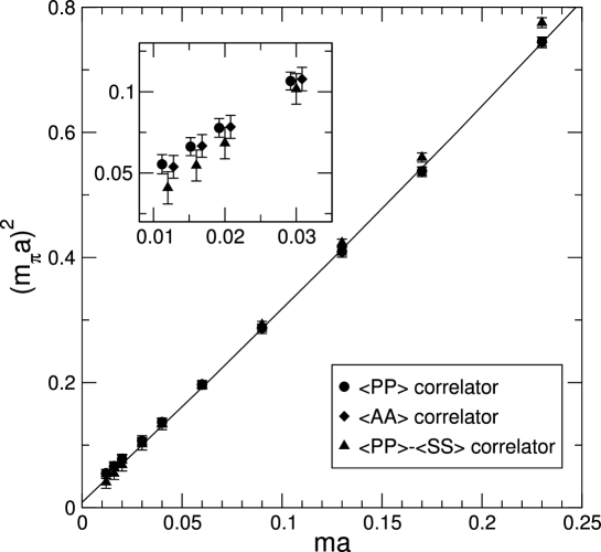
Figure 11: Squared pion mass for the overlap-improved FP Dirac operator $D^{\rm FP}_{\rm ov}$ from 28 $9^{3}\times 24$ gauge configurations at lattice spacing $0.16\,{\rm fm}$, with a quadratic fit to the P correlator at large and the P-S correlator at small quark mass. The inset shows the smallest four masses on a magnified scale.

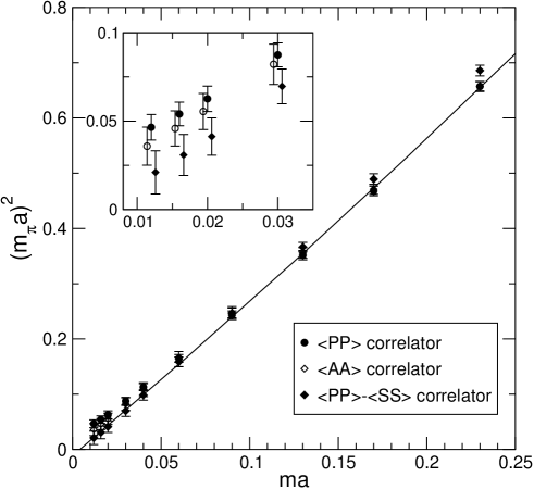
Figure 12: Squared pion mass for the overlap-improved FP Dirac operator $D^{\rm FP}_{\rm ov}$ from 32 $9^{3}\times 24$ gauge configurations at lattice spacing $0.13\,{\rm fm}$, with a quadratic fit to the P correlator at large and the P-S correlator at small quark mass. The inset shows the smallest four masses on a magnified scale.

For spectroscopy we approximate the inverse square root $1/\sqrt{A^{\dagger}A}$ with a polynomial of order 3, projecting out the smallest 20 eigenvalues of $A^{\dagger}A$ for faster convergence. The improved chiral behaviour allows the quark mass to be decreased even further. The smallest input quark mass we considered is $ma=0.012$ where the pion to rho mass ratio is $m_{\pi}/m_{\rho}=0.27(4)$ and $0.24(7)$ at lattice spacings $0.16$ and $0.13\,{\rm fm}$ respectively (Tables 5 and 6). In Figs. 11 and 12, we show the pion mass squared measured using the overlap-improved FP Dirac operator. For an exactly chiral action, the topological finite-volume effects cancel exactly for the P-S correlator. A quadratic fit to the squared pion mass is consistent with zero at $m=0$ within the large error at this small number of gauge configurations.

4.2 Chiral condensate ${\mathbf{\langle}\overline{\Psi}\Psi\rangle}$

It is the common expectation that for QCD with a number $N_{f}\geq 2$ of massless quark flavours, the chiral symmetry is spontaneously broken by a non-zero expectation value for the chiral condensate $\langle\overline{\Psi}\Psi\rangle$. Chiral perturbation theory ($\chi{\rm PT}$), which is based on this assumption, is an excellent description of many low-energy QCD phenomena [38]. However, it is only possible via lattice QCD to test from first principles if the symmetry is spontaneously broken.

The leading order effective theory of $\chi{\rm PT}$ contains the low energy constants $f_{\pi}$ and $\Sigma$. In full QCD the Gell-Mann-Oakes-Renner relation

$$f_{\pi}^{2}m_{\pi}^{2}=4m\Sigma,$$ (10)

becomes exact in the $m\rightarrow 0$ chiral limit and the chiral condensate $\langle\overline{\Psi}\Psi\rangle=\langle\bar{u}u\rangle=\langle\bar{d}d\rangle=\dots$, defined at zero quark mass, is equal to -$\Sigma$. The low energy constant $\Sigma$ depends on the number of massless flavours $N_{f}$.

In quenched QCD ($N_{f}=0$), the relation $\langle\overline{\Psi}\Psi\rangle=-\Sigma$ and Eq. (10) receive corrections even in the chiral limit [39, 40]. Actually, $\langle\overline{\Psi}\Psi\rangle$ and $m_{\pi}^{2}/m$ in the chiral limit are not defined due to diverging quenched chiral logarithms. This expectation seems to be confirmed in numerical studies of the Banks-Casher relation [41].

On the other hand, it is possible to study and determine the low energy constant $\Sigma(N_{f}=0)$ in the quenched theory. Under the assumption that $\Sigma(N_{f})$ is a smooth function of $N_{f}$ and $\Sigma(N_{f}=0)$ is close to $\Sigma(N_{f}=3)$ (which is the standard assumption when quenched results are used to estimate full QCD quantities) we get an estimate for the chiral condensate $-\langle\overline{\Psi}\Psi\rangle(N_{f}=3)=\Sigma(N_{f}=3)\approx\Sigma(N_{f}=0)$.

One possibility to determine $\Sigma(N_{f}=0)$ is to study the chiral condensate in a fixed topological sector with charge $Q$ in a finite volume $V$ at finite quark mass $m$ [40]. The volume and the quark mass are chosen so that the finite size effects are dominated by the pions with zero momentum. Using $\chi{\rm PT}$, or random matrix theory, the fermion condensate at finite volume and quark mass has been calculated in the continuum, both for full and quenched QCD. The quenched QCD condensate $\langle\overline{\Psi}\Psi\rangle_{m,V,Q}$ is given by

$$-\langle\overline{\Psi}\Psi\rangle_{m,V,Q}=mV\Sigma^{2}[I_{|Q|}(z)K_{|Q|}(z)+I_{|Q|+1}(z)K_{|Q|-1}(z)]+\frac{|Q|}{mV}\,,$$ (11)

where $I_{Q}$ and $K_{Q}$ are modified Bessel functions, $z=m\Sigma V$ and the $N_{f}=0$, $V=\infty$, $m=0$ low energy constant $\Sigma$ is the quantity we wish to measure. By measuring $\langle\overline{\Psi}\Psi\rangle_{m,V,Q}$ in different topological sectors at different masses and volumes, the continuum prediction of the $m$ and $V$ dependence can be used to extract $\Sigma$.

On the lattice we calculate the bare subtracted condensate by measuring the trace

$$-\langle\overline{\Psi}\Psi\rangle_{m,V,Q}^{\rm sub} =\frac{1}{V}\Big{\langle}{\rm Tr}^{\prime}\Big{[}(D(m)2R)^{-1}-\frac{1}{2}D(0)D^{-1}(m)\Big{]}\Big{\rangle}$$

$$=\frac{1}{V}\frac{1}{1-\frac{m}{2}}\Big{\langle}{\rm Tr}^{\prime}\Big{[}(D(m)2R)^{-1}-\frac{1}{2}\Big{]}\Big{\rangle}\,,$$ (12)

where $D$ and $R$ are related via the Ginsparg-Wilson relation and where we make use of Eq. (7) to simplify the expression on the first line. Notice that in order to keep the conventional notation we use $\langle\overline{\Psi}\Psi\rangle_{m,V,Q}^{\rm sub}$ in Eq. (12) even though we actually measure the expectation value of the scalar density $S^{0}$ as defined in Eq. (53), which differs from $\langle\overline{\Psi}\Psi\rangle_{m,V,Q}^{\rm sub}$ by a tree level factor that will finally drop out in the renormalized value for $\Sigma$. We measure the trace stochastically using random $Z(2)$ vectors [42]. In order to measure the condensate at very small quark mass, the remnant explicit chiral symmetry breaking must be very small, so we use the overlap-improved operator $D_{\rm ov}^{\rm FP}$, where $D^{\rm FP}$ is taken as input. Due to the $|Q|$ chiral zero modes of the Dirac operator, the quenched condensate contains a term $|Q|/(mV)$ which diverges as the mass becomes small. In the volumes we study, the $|Q|$ zero modes always have the same chirality and their contribution to the condensate is removed by measuring the trace ${\rm Tr}^{\prime}$ in the chiral sector opposite to the zero modes [43, 44], i.e. if the $|Q|$ modes have chirality $+$, the $Z(2)$ vectors used to measure the trace are chosen to have chirality $-$. To determine $\langle\overline{\Psi}\Psi\rangle_{m,V,Q}^{\rm sub}$, the stochastic trace is doubled to include both chiral sectors.

We first generated ensembles of gauge configurations at different volumes. We determined the topological charge $Q$ of the configurations from the chirality of the lowest eigenmodes of $(D^{\rm FP}_{\rm ov})^{\dagger}D^{\rm FP}_{\rm ov}$, which we find with an Arnoldi solver [45]. To scan for the topology, a Legendre polynomial of order 2 is used to approximate $1/\sqrt{A^{\dagger}A}$, projecting out the 10 smallest $A^{\dagger}A$ eigenvalues. This is sufficiently accurate to determine the chirality of the eigenmodes to better than $1\%$ accuracy.

$L$	order	$|Q|$	$N_{\rm conf}$
8	7	1	154
		2	41
10	10	1	53
		2	43

Table 7: Polynomial order of $1/\sqrt{A^{\dagger}A}$ approximation and statistics for the condensate measurement.

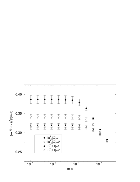
Figure 13: The ratio $(-\langle\overline{\Psi}\Psi\rangle_{m,V,Q}^{\rm sub}a^{3})/(ma)$ versus $ma$ for different volumes and topological sectors.

We have measured the condensate in volumes $8^{4}$ and $10^{4}$ at lattice spacing $0.13\,{\rm fm}$ (corresponding to the bare coupling $\beta=3.2$). We use 10 random $Z(2)$ vectors to measure the trace for each configuration and a BiCGstab multi-mass solver to invert $D_{\rm ov}^{\rm FP}$ at all masses simultaneously. In the overlap operator, we approximate $1/\sqrt{A^{\dagger}A}$ with Legendre polynomials of order 7 and 10 for volumes $8^{4}$ and $10^{4}$, respectively. This gives sufficiently precise chiral symmetry — increasing the polynomial order further, the relative change in $(\langle\overline{\Psi}\Psi\rangle_{m,V,Q}^{\rm sub}a^{3})/(ma)$ is $\leq{\cal O}(10^{-4})$. We project out the 10 smallest $A^{\dagger}A$ eigenvalues, which are treated exactly. Our statistics are given in Table 7. In Fig. 13, we plot $(-\langle\overline{\Psi}\Psi\rangle_{m,V,Q}^{\rm sub}a^{3})/(ma)$ as a function of $ma$ for the different volumes and topological sectors.

The bare quark condensate at finite quark mass contains a $\sim m/a^{2}$ cut-off effect. As the quark mass $m\rightarrow 0$,

$$-\frac{\langle\overline{\Psi}\Psi\rangle_{m,V,Q}^{\rm sub}}{m}=\frac{\Sigma^{2}V}{2|Q|}+\frac{c_{1}}{a^{2}},$$ (13)

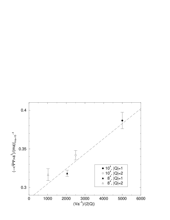
Figure 14: The ratio $(-\langle\overline{\Psi}\Psi\rangle_{m,V,Q}^{\rm sub}a^{3})/(ma)$ at $ma=10^{-4}$ versus $V/(2|Q|)$. The dashed line is a $\chi^{2}$-fit.

where $c_{1}$ is an unknown coefficient which has to be fitted. As the coefficient $c_{1}$ comes from ultraviolet fluctuations, it is natural to assume that it is independent of the topological charge $Q$. The contribution of the $|Q|$ zero modes has been removed, and there is no artifact $1/(ma^{3})$ in Eq. (13) due to the fact that the condensate is defined as the expectation value of a scalar operator which transforms covariantly under chiral transformations and has no mixing with the unit operator. (For further discussions, see Sec. 5.) From Fig. 13, we see that $(-\langle\overline{\Psi}\Psi\rangle_{m,V,Q}^{\rm sub}a^{3})/(ma)$ reaches a plateau at very small quark mass. In Fig. 14, we plot the value of $(-\langle\overline{\Psi}\Psi\rangle_{m,V,Q}^{\rm sub}a^{3})/(ma)$ at $ma=10^{-4}$ versus $V/(2|Q|)$, which we fit to the form of Eq. (13). From the slope, we extract the bare low energy constant as $a^{3}\Sigma=4.42(36)\times 10^{-3}$. We convert this using the Sommer parameter ($r_{0}/a=3.943(60)$ has previously been measured at this lattice spacing), giving $r_{0}^{3}\Sigma=0.271(22)(12)$, where the first error is statistical and the second the uncertainty in the scale.

In order to turn this bare result into the renormalized low energy constant we need the scalar renormalization factor $Z_{S}$. In the present test study we obtained $Z_{S}$ combining the continuum extrapolated renormalization group invariant (RGI) quark mass of the ALPHA collaboration [48] with our spectroscopy data in Sect. 4.1. This method has been suggested recently by Hernández et al. [49].

Chiral symmetry connects the scalar and pseudoscalar renormalization factors: $Z_{P}=Z_{S}=1/Z_{m}$, where $Z_{m}$ is the multiplicative mass renormalization. This way the problem is reduced to finding $Z_{m}$. The technique requires the measurement of the pion mass at a number of quark masses. The renormalization factor $Z_{m}$ connecting our quark mass $m$ to the RGI mass M defined at some reference pion mass $m_{\pi}$ is given by

$$Z_{m}=\left.\frac{U_{M}}{r_{0}m}\right|_{(r_{0}m_{\pi})^{2}=x_{\rm ref}},$$ (14)

where $U_{M}=r_{0}M$. The renormalization factor $Z_{m}$ should be independent of the reference point, so finding this ratio at a number of pseudoscalar masses indicates the systematic error. We have performed mass measurements at two lattice spacings corresponding to $\beta=3.0$ and $3.2$. We use the same reference points and values of $U_{M}$ as in [49] to determine $Z_{m}$. The results are summarized below in Table 8.

$\beta$	$x_{\rm ref}$	$U_{M}$	$r_{0}m$	$Z_{m}$
3.0	1.5736	0.181(6)	0.156(4)	1.16(5)
	3.0	0.349(9)	0.296(8)	1.18(5)
	5.0	0.580(12)	0.490(14)	1.18(4)
3.2	1.5736	0.181(6)	0.141(27)	1.28(25)
	3.0	0.349(9)	0.271(24)	1.29(12)
	5.0	0.580(12)	0.446(22)	1.30(7)

Table 8: The renormalization factor $Z_{m}$ determined at different lattice spacings and reference pseudoscalar masses.

At each lattice spacing, the values for $Z_{m}$ at the different reference points are in very good agreement with one another. We take the average of the values and the error at $x_{\rm ref}=3.0$ as our determination of $Z_{m}$. The renormalization group invariant low energy constant is $\hat{\Sigma}=Z_{S}\Sigma$. To convert this result into the $\overline{\rm MS}$ scheme, we use the fact that

$$\frac{\hat{\Sigma}}{\Sigma_{\overline{\rm MS}}(2\,{\rm GeV})}=\frac{\overline{m}_{\overline{\rm MS}}(2\,{\rm GeV})}{M}=0.72076,$$ (15)

where the ratio of masses has been calculated perturbatively to four loops in the $\overline{\rm MS}$ scheme [50].

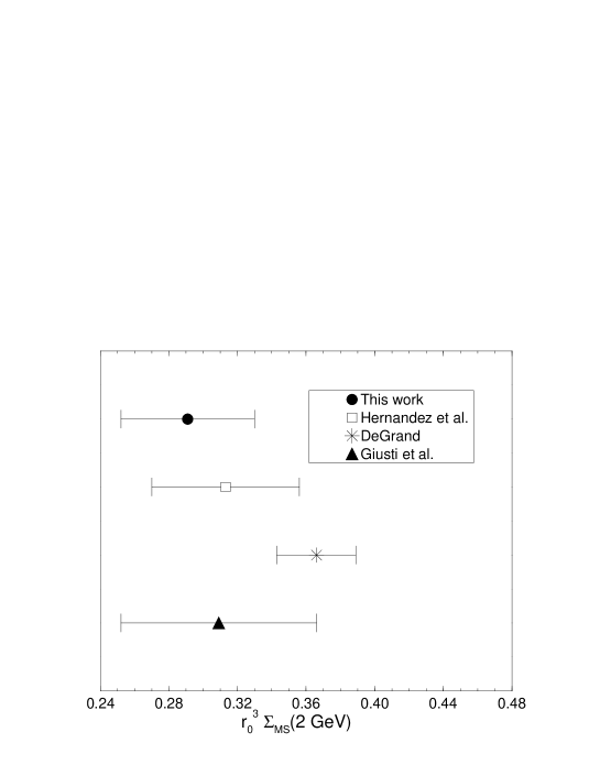
Figure 15: Comparison of different measurements of $r_{0}^{3}\Sigma_{\overline{\rm MS}}(2\,{\rm GeV})$.

Taking the renormalization factor $Z_{S}=1/Z_{m}=0.78(7)$ at $\beta=3.2$, where the bare $\Sigma$ is obtained, we get for the renormalization group invariant low energy constant $r_{0}^{3}\hat{\Sigma}=0.210(17)(9)(20)$, with statistical, scale and renormalization errors respectively. Taking $r_{0}=0.5\,{\rm fm}$ and combining the errors in quadrature, this corresponds to $\hat{\Sigma}=(235\pm 11\,{\rm MeV})^{3}$. We can also convert this result to the $\overline{\rm MS}$ scheme giving $\Sigma_{\overline{\rm MS}}(2\,{\rm GeV})=(262\pm 12\,{\rm MeV})^{3}$. As Fig. 15 illustrates, our measurement of the renormalized chiral condensate is in good agreement with other recent determinations [36, 44, 51].

4.3 Alternative determinations of the chiral condensate

A direct determination of $\Sigma$ discussed above is only possible with a chirally symmetric action. An alternative, more phenomenological way is to use the GMOR relation, Eq. (10) using the pion mass measurements and the experimental value of $f_{\pi}$ [34, 35, 36]. Although the ratio $m_{\pi}^{2}/m_{q}$ is not defined in the quenched theory in the chiral limit $m_{q}\rightarrow 0$, due to quenched chiral logarithms, we see that the pion mass squared is consistent with linear behavior for intermediate quark mass. Assuming that the chiral logarithms have very little effect in this mass range, we identify the slope $B_{M}$ as $4\Sigma/f_{\pi}^{2}$. Table 9 gives the value of the slope $B_{M}$ and the bare condensate $a^{3}\Sigma$ calculated through the GMOR relation, $\Sigma=B_{M}f_{\pi}^{2}/4$, using the physical value $f_{\pi}=131\,{\rm MeV}$. The value at $\beta=3.2$, $a^{3}\Sigma=5.8(2)\times 10^{-3}$ has to be compared with the direct measurement discussed above, which gave $4.4(4)\times 10^{-3}$.

$\beta$	$a$[fm]	$B_{M}$	$a^{3}\Sigma\times 10^{3}$
3.0	0.16	3.22(12)	8.8(3)
3.2	0.13	2.90(12)	5.8(2)

Table 9: The value of the bare chiral condensate determined from pion mass measurements. The slope $B_{M}$ of $m_{\pi}^{2}$ vs. $m_{q}$, and the value of the bare chiral condensate determined from GMOR relation, with $f_{\pi}=131\,{\rm MeV}$.

We have to mention a difficulty with the technique used in the direct determination of the condensate discussed in the previous subsection. Finding the finite-volume behavior of the trace in Eq. (12), the major problem is from rare, but very large contributions to the average. These come from configurations where the Dirac operator has very small, but non-zero, eigenvalues. Due to their presence, we found it difficult to control the statistical error. The distribution of the low-lying eigenvalues of the Dirac operator offers an alternative method to determine $\Sigma$ [52]. This method does not suffer from the problem mentioned above. The appearance of very small eigenvalues does not bring any large contributions, which might make this method competitive, or even better than the finite-volume technique.

To compare techniques of measuring the low energy constant $\Sigma$, we performed a test study of the distribution of low-lying eigenvalues of the Dirac operator. We generated ensembles of $4^{4}$ lattice volume, with 2000 gauge configurations at $\beta=2.4$ (lattice spacing $0.30\,{\rm fm}$) and 1000 configurations at $\beta=2.7$ (lattice spacing $0.22\,{\rm fm}$). Admittedly, this lattice volume is too small and the resolutions are too coarse to allow a serious study of the low lying eigenvalues. Using the Ritz functional method, we measured the smallest non-zero eigenvalue of $D_{\rm ov}^{\rm FP}$ and determined the smallest eigenvalue distribution for each topological sector. For the overlap-improved operator, we used an order 5 polynomial approximation of $1/\sqrt{A^{\dagger}A}$, with the smallest 20 and 8 $A^{\dagger}A$ eigenvalues projected out at $\beta=2.4$ and 2.7 respectively. Even on these coarse lattices, this low-order approximation has very little chiral symmetry breaking. Using random matrix theory, the distribution of the smallest eigenvalue $\lambda$ in topological sector $Q$ in the quenched theory is

$$P(z) = \frac{z}{2}e^{-z^{2}/4}~{}{\rm det}[I_{2+i-j}(z)]\hskip 28.45274pti,j=1,...,|Q|$$

$$P(z) = \frac{z}{2}e^{-z^{2}/4}\hskip 91.04872ptQ=0,$$ (16)

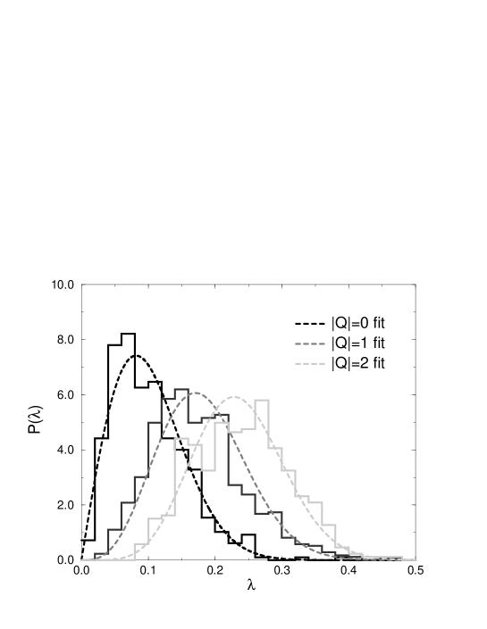
Figure 16: Distributions of the smallest eigenvalue $\lambda$ of $D^{\rm FP}_{\rm ov}$ for topological sectors $|Q|=0,1,2$, volumes $4^{4}$ at lattice spacing $0.30\,{\rm fm}$. The curves are the random matrix theory fit to the histograms.

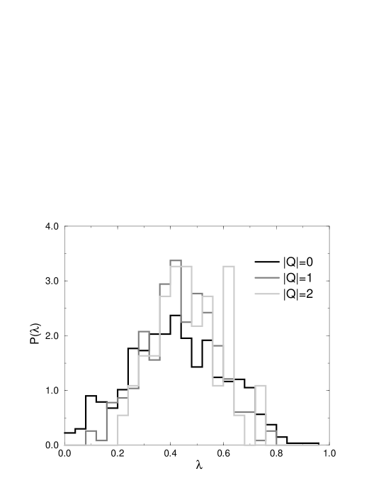
Figure 17: Distributions as in Fig. 16 for volumes $4^{4}$ at lattice spacing $0.22\,{\rm fm}$.

where $z=\lambda\Sigma V$ is the rescaled eigenvalue and $I_{k}$ are the modified Bessel functions. In Fig. 16, we plot the measured distributions for topological sectors $|Q|=0,1,2$ at $\beta=2.4$, as well as the fits to the predicted form. We see the fits describe the data quite well, allowing us to estimate the bare quantity $a^{3}\Sigma=0.0687(27)$, or alternatively $r_{0}^{3}\Sigma=0.332(16)$. In Fig. 17, however, we see that the smallest eigenvalue distributions at $\beta=2.7$ for different topological sectors lie on top of one another and are clearly not described by Eq. (4.3). The extreme values of $\beta$ and/or lattice size ($L=4$) might be the reason for this result. Further studies are needed to clarify this point.

4.4 The quenched topological susceptibility

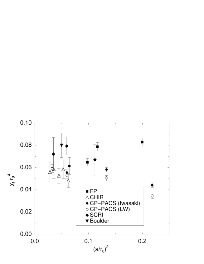
Figure 18: The quenched topological susceptibility measured by different actions and techniques. The CP-PACS data are obtained by cooling using the Iwasaki and the Lüscher-Weisz actions (see [46]). The other data are obtained by chirally symmetric actions. FP denotes the present determination using $D_{\rm ov}^{\rm FP}$. The others are obtained using a chirally improved action [47](CHIR), the overlap with the Wilson action [63](SCRI) and the overlap with the planar action [64, 62](Boulder).

As discussed above, in the course of measuring the quark condensate we have determined the topological charge of the gauge configurations from the chirality of the lowest eigenmodes of $(D^{\rm FP}_{\rm ov})^{\dagger}D^{\rm FP}_{\rm ov}$. As a byproduct, we obtain the quenched topological susceptibility $\chi_{t}=\langle Q^{2}\rangle/V$ from the distribution of the topological charge. From an ensemble of 200 $\,10^{4}$ configurations at our smallest lattice spacing $0.13\,{\rm fm}$, we find $r_{0}^{4}\chi_{t}=0.0612(75)$, corresponding to $\chi_{t}=(196\pm 6\,{\rm MeV})^{4}$. This result, which still might have sizeable cut-off effects, is consistent with earlier determinations, as shown in fig. 18.

4.5 Local chirality of near-zero modes

Exact zero modes of the Dirac operator tell us, via the index theorem, about the topological charge $Q$ of the background gauge configuration. However, the exact zero modes alone cannot break chiral symmetry spontaneously. According to the Banks-Casher relation [53] $\langle\overline{\Psi}\Psi\rangle=-\pi\rho(0)\neq 0$, the Dirac operator must build up a finite density of near-zero modes, which does not vanish as $V\rightarrow\infty$.

One mechanism which explains the formation of near-zero modes involves instantons. Consider a gauge configuration containing one instanton and one anti-instanton. If the instanton and anti-instanton are separated by a large distance, the Dirac operator has a pair of complex eigenvalues lying close to 0. The farther the instanton and anti-instanton are separated from each other, the closer the complex eigenvalue pair moves to the origin. If the instanton and anti-instanton are brought closer together, the complex eigenvalue pair moves away from the origin and disappears into the bulk of the eigenvalue spectrum. If the gauge configurations contain many instantons and anti-instantons, this could produce a non-zero density of near-zero modes, giving $\rho(0)\neq 0$ in the infinite volume limit.

The question has recently been raised if it is possible to show that the near-zero modes are dominated by instantons. From instanton physics, it is expected that the modes are highly localized where the instantons and anti-instantons sit. If this is so, then in these regions the modes should be close to chiral i.e. mostly either left- or right-handed, depending on whether it is sitting on an instanton or anti-instanton. In [54], the authors defined a measure of local chirality at lattice site $x$ by

$$\tan\left[\frac{\pi}{4}(1+X(x))\right]=\sqrt{\frac{{\Psi_{\rm L}}^{\dagger}\Psi_{\rm L}(x)}{{\Psi_{\rm R}}^{\dagger}\Psi_{\rm R}(x)}},$$ (17)

where $\Psi_{\rm L/R}(x)$ are the standard ${\rm L/R}$ projections of the corresponding wave function. An exact zero mode is purely either left- or right-handed, giving $X(x)=\pm 1$ at all lattice sites $x$. If a near-zero mode is localized around instanton-anti-instanton lumps, then $X(x)$ should be close to $\pm 1$ for the sites $x$ where the probability density $\Psi^{\dagger}\Psi(x)$ is largest.

In the original paper [54], many near-zero modes of the Wilson operator $D^{\rm W}$ were analysed for many gauge configurations and the finding was that in the regions where the modes are localized, the distribution for $X(x)$ is peaked around 0 and the modes do not display local chirality. This led to the conclusion that the near-zero modes are not dominated by instantons. Since then, several other groups have found the opposite conclusion [55], using a Dirac operator with much better chiral symmetry than $D^{\rm W}$ (or even just an alternative definition of a complete basis for the non-normal operator $D^{\rm W}$). They find the distribution of $X(x)$ is double-peaked with maxima at large positive and negative values of $X$, indicating that the modes are locally chiral. On the other hand, in several more detailed comparisons the semiclassical expectations were not confirmed by the numerical data[56]. Presumably, one must not take this picture too seriously in a situation where these objects do not form a dilute gas and live in a strongly fluctuating background.

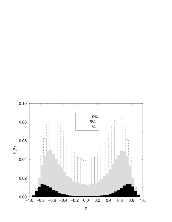
Figure 19: The distribution $P(X)$ for volumes $10^{4}$ at lattice spacing $0.13\,{\rm fm}$. We include the top 1%, 5% and 10% lattice sites with largest density $\Psi^{\dagger}\Psi(x)$.

We have analyzed the 10 smallest near-zero modes of the overlap-improved $D_{\rm ov}^{\rm FP}$ for 60 $10^{4}$ gauge configurations at lattice spacing $0.13\,{\rm fm}$. We use a Legendre polynomial of order 2 to approximate $1/\sqrt{A^{\dagger}A}$ in $D_{\rm ov}^{\rm FP}$, with the 10 smallest $A^{\dagger}A$ being projected out and treated exactly. The eigenvalues and eigenvectors are found using the Arnoldi solver. In Fig. 19, we plot the distribution $P(X)$ of the measure of local chirality $X$ at the lattice sites where the density $\Psi^{\dagger}\Psi(x)$ of a mode is largest. The three distributions correspond to taking, for each mode, 1%, 5% and 10% of all lattice sites which have the largest density $\Psi^{\dagger}\Psi(x)$. We do not include exact zero modes, for which $X(x)=\pm 1$ at all lattice sites. We see a very clear double-peaked distribution, whose maxima are farther from zero if we only include the sites where the modes are most localized. The maxima are not at $X=\pm 1$ as the modes are not exactly chiral. We find the same conclusion as [55] — where the near-zero modes are most localized, they are also very chiral. Recent work [57] has shown that at the places where the near-zero modes of the Dirac operator are concentrated, the gauge field appears to contain lumps of $F\tilde{F}$. This behavior is consistent with the picture of instanton-dominance of the near-zero modes, however it is not a conclusive evidence that instantons are the driving mechanism for chiral symmetry breaking.

5 Covariant densities and conserved currents

The GW relation

$${\gamma_{5}}D+D{\gamma_{5}}=D{\gamma_{5}}D\,.$$ (18)

implies an exact SU($N_{f}$) $\times$ SU($N_{f}$) global symmetry on the lattice [12]. The vector transformation reads

$$\delta_{V}^{a}\psi=i\epsilon T^{a}\psi\,,\qquad\delta_{V}^{a}\overline{\psi}=-i\overline{\psi}T^{a}\epsilon\,,$$ (19)

while the axial transformation has the form

$$\delta_{A}^{a}\psi=i\epsilon T^{a}{\hat{\gamma}_{5}}\psi\,,\qquad\delta_{A}^{a}\overline{\psi}=i\overline{\psi}{\gamma_{5}}T^{a}\epsilon\,,$$ (20)

where $T^{a}$, $a=1,\ldots,N_{f}^{2}-1$ are SU($N_{f}$) generators

$$[T^{a},T^{b}]=if_{abc}T^{c}\,,\qquad{\rm tr}\left(T^{a}T^{b}\right)=\frac{1}{2}\delta^{ab}\,,$$ (21)

and

$${\hat{\gamma}_{5}}={\gamma_{5}}(1-D)\,.$$ (22)

The action

$${\cal A}=\overline{\psi}D(U)\psi$$ (23)

is invariant under these transformations if $D(U)$ satisfies Eq. (18). The fact that ${\cal A}$ is a scalar under the transformations in Eqs. (19) and (20) implies also that it is ${\cal O}(a)$ improved since the mixing of the action density with other dim=5 operators (in particular, with the clover term) is forbidden by the symmetries. The spectral quantities are therefore automatically ${\cal O}(a)$ improved.

The exact global symmetries above imply the existence of conserved currents. The form of the conserved currents is not unique. It is very useful to work with conserved currents and scalar and pseudoscalar densities which transform covariantly (i.e. the same way as in the formal continuum) under the global transformations in Eqs. (19) and (20). These dim=3 operators are again automatically ${\cal O}(a)$ improved: there are no dim=4 operators they can mix with.

Our way to find chiral covariant conserved currents is the same as that proposed by Kikukawa and Yamada [58] who presented explicitly the vector and axial currents in the overlap construction with Wilson kernel. We present here the currents in the general case in a form which, we believe, is easy to use in numerical simulations. We discuss the scalar and pseudoscalar densities, the Ward identities and the case $2R\neq 1$ also. In the Appendices we collect some of the identities implied by the GW relation.

5.1 A useful form of the currents

Consider a global transformation $\psi\to\psi+\delta\psi$, $\overline{\psi}\to\overline{\psi}+\delta\overline{\psi}$ and assume that the action Eq. (23) is invariant under this transformation, $\delta{\cal A}=0$. Assume that under the corresponding local transformation the change of the action can be written in the form

$$\delta{\cal A}=i\overline{\psi}A(U)[D(U),\epsilon]B(U)\psi\,,$$ (24)

where, for notational convenience, we treat the infinitesimal, $x$-dependent parameter of the transformation as a diagonal matrix

$$\left(\epsilon\right)_{xy}=\epsilon(x)\delta_{xy}\,.$$ (25)

We shall consider the case where $A(U)$ and $B(U)$ transform correctly under a gauge transformation to make $\delta{\cal A}$ gauge invariant. The corresponding current is defined through

$$\delta{\cal A}=i\sum_{x}\partial_{\mu}\epsilon(x)J_{\mu}(x)=-i\sum_{x}\epsilon(x)\partial_{\mu}^{*}J_{\mu}(x)\,,$$ (26)

where $\partial_{\mu}$ and $\partial_{\mu}^{*}$ are the forward and backward lattice derivatives respectively.

Consider first the case $A=B=1$, the generalization is trivial. We extend the gauge fields from $\mathrm{SU}(N_{c})$ to $\mathrm{SU}(N_{c})\times\mathrm{U}(1)$ maintaining the gauge covariance of $D(U)$. Consider a $\mathrm{U}(1)$ gauge transformation

$$U_{\mu}(x)\to\tilde{U}_{\mu}(x)=\mathrm{e}^{i\epsilon(x)}U_{\mu}(x)\mathrm{e}^{-i\epsilon(x+\hat{\mu})}\,.$$ (27)

For this we have

$$D(U)_{yz}\to D(\tilde{U})_{yz}=\mathrm{e}^{i\epsilon(y)}D(U)_{yz}\mathrm{e}^{-i\epsilon(z)}\,,$$ (28)

i.e. for an infinitesimal U(1) gauge transformation the change of $D(U)$ is given by

$$\delta_{\mathrm{g}}D(U)=-i[D(U),\epsilon]\,.$$ (29)

Using Eqs. (24) and (26) one has

$$\delta{\cal A}=i\sum_{x}\partial_{\mu}\epsilon(x)J_{\mu}(x)=-\overline{\psi}\delta_{\mathrm{g}}D(U)\psi\,.$$ (30)

We show below that $\delta_{\mathrm{g}}D(U)$ can be rewritten in the form

$$\delta_{\mathrm{g}}D(U)=-i\sum_{x}\partial_{\mu}\epsilon(x)K_{\mu}(x)\,,$$ (31)

which gives then

$$J_{\mu}(x)=\overline{\psi}K_{\mu}(x)\psi\equiv\sum_{yz}\overline{\psi}_{y}(K_{\mu}(x))_{yz}\psi_{z}\,.$$ (32)

To construct $K_{\mu}(x)$ satisfying Eq. (31) observe that the gauge transformation in Eq. (28) can be reached by performing the changes

$$U_{\mu}(x)\to U_{\mu}^{(\alpha)}(x)=\mathrm{e}^{i\alpha_{\mu}(x)}U_{\mu}(x)$$ (33)

on each link independently and taking the actual values of $\alpha_{\mu}(x)$ to be

$$\alpha_{\mu}(x)=-\partial_{\mu}\epsilon(x)\,.$$ (34)

(Note that the individual changes in Eq.(33) are not pure gauge transformations – they only add up to that after all the links have been properly changed.)

To linear order we have

$$\delta_{\mathrm{g}}D(U)=D(\tilde{U})-D(U)=-\sum_{x}\partial_{\mu}\epsilon(x)\left.\frac{\delta D(U_{\mu}^{(\alpha)})}{\delta\alpha_{\mu}(x)}\right|_{\alpha=0}\,.$$ (35)

Eqs. (31) and  (35) give the kernel of the current:

$$K_{\mu}(x)=-i\left.\frac{\delta D(U_{\mu}^{(\alpha)})}{\delta\alpha_{\mu}(x)}\right|_{\alpha=0}\,.$$ (36)

It is easy to see that in the general case of Eq. (24) the current is given by the kernel

$$\tilde{K}_{\mu}(x)=A(U)K_{\mu}(x;U)B(U)\,,$$ (37)

where $K_{\mu}(x)$ is defined in Eq. (36). Observe that Eq. (36) provides a straightforward way for practical determination of the kernel $K_{\mu}(x)$ (and hence of the conserved currents discussed below) by performing the numerical differentiation in $\alpha_{\mu}(x)$.

5.2 Chiral covariant conserved vector and axial currents

Consider a global chiral transformation acting only on the right-handed components $\psi_{R}=\hat{P}_{R}\psi$ and $\overline{\psi}_{R}=\overline{\psi}P_{L}$ :

$$\delta_{R}^{a}\psi=i\epsilon T^{a}\hat{P}_{R}\psi\,,\qquad\delta_{R}^{a}\overline{\psi}=-i\overline{\psi}P_{L}T^{a}\epsilon\qquad\text{(global)}\,,$$ (38)

and the analogous global left-handed transformations

$$\delta_{L}^{a}\psi=i\epsilon T^{a}\hat{P}_{L}\psi\,,\qquad\delta_{L}^{a}\overline{\psi}=-i\overline{\psi}P_{R}T^{a}\epsilon\,,\qquad\text{(global)}\,.$$ (39)

The projectors above are defined as [13, 59]

$$\hat{P}_{R/L}=\frac{1}{2}(1\pm{\hat{\gamma}_{5}})\,,\qquad P_{R/L}=\frac{1}{2}(1\pm{\gamma_{5}})\,.$$ (40)

These transformations are symmetries of the action. It is convenient to promote these global transformations to local ones in a way preserving chirality [58],

$$\delta_{R}^{a}\psi=iT^{a}\hat{P}_{R}\epsilon\hat{P}_{R}\psi\,,\qquad\delta_{R}^{a}\overline{\psi}=-i\overline{\psi}P_{L}\epsilon P_{L}T^{a}\,.$$ (41)

In Eq. (41) $\epsilon\hat{P}_{R}\psi$ is not a right-handed field if $\epsilon$ is $x$-dependent. This explains the presence of the second projector $\hat{P}_{R}$ [58]. Keeping the form of Eqs. (38), (39) in the local case would produce conserved currents as well, transforming, however, non-covariantly under global transformations. Note that it is preferable to use the covariant conserved current. For example, the pion is created from the vacuum by the covariant current, and the corresponding relation defining $f_{\pi}$ is valid for this current. Non-covariant conserved currents result in an extra $m$-dependent factor (cf. Appendix C).

Using the identity $D\hat{P}_{R}=P_{L}D$ one can write the corresponding change of the action as

$$\delta_{R}^{a}{\cal A}=i\overline{\psi}\left(P_{L}[D,\epsilon]\hat{P}_{R}T^{a}\right)\psi\,.$$ (42)

This is of the general form considered in Eq. (24) hence we readily obtain the corresponding current

$$J_{R\mu}^{a}(x)=\overline{\psi}K_{R\mu}^{a}(x)\psi\,,\qquad K_{R\mu}^{a}(x)=P_{L}K_{\mu}(x)\hat{P}_{R}T^{a}\,,$$ (43)

where the kernel $K_{\mu}(x)$ is defined in Eq. (36).

Similarly, the left-handed local transformation is

$$\delta_{L}^{a}\psi=iT^{a}\hat{P}_{L}\epsilon\hat{P}_{L}\psi\,,\qquad\delta_{L}^{a}\overline{\psi}=-i\overline{\psi}P_{R}\epsilon P_{R}T^{a}\,.$$ (44)

and the left-handed current is given by

$$J_{L\mu}^{a}(x)=\overline{\psi}K_{L\mu}^{a}(x)\psi\,,\qquad K_{L\mu}^{a}(x)=P_{R}K_{\mu}(x)\hat{P}_{L}T^{a}\,.$$ (45)

Under the global chiral transformations in Eqs. (38) and (39) these currents transform covariantly

$$\frac{i}{\epsilon}\delta_{R}^{a}J_{R\mu}^{b}(x)=if_{abc}J_{R\mu}^{c}(x)\,,\qquad\frac{i}{\epsilon}\delta_{L}^{a}J_{L\mu}^{b}(x)=if_{abc}J_{L\mu}^{c}(x)\,.$$ (46)

The currents $J_{R\mu}$ and $J_{L\mu}$ are, of course, invariant under the left- and right-handed transformations, respectively. These properties imply that the vector and axial currents

$$\begin{split}V_{\mu}^{a}(x)=J_{R\mu}^{a}(x)+J_{L\mu}^{a}(x)&=\overline{\psi}\left(P_{L}K_{\mu}(x)\hat{P}_{R}+P_{R}K_{\mu}(x)\hat{P}_{L}\right)T^{a}\psi\\ &=\frac{1}{2}\overline{\psi}\left(K_{\mu}(x)-{\gamma_{5}}K_{\mu}(x){\hat{\gamma}_{5}}\right)T^{a}\psi\,,\end{split}$$ (47)

$$\begin{split}A_{\mu}^{a}(x)=J_{R\mu}^{a}(x)-J_{L\mu}^{a}(x)&=\overline{\psi}\left(P_{L}K_{\mu}(x)\hat{P}_{R}-P_{R}K_{\mu}(x)\hat{P}_{L}\right)T^{a}\psi\\ &=\frac{1}{2}\overline{\psi}\left(-{\gamma_{5}}K_{\mu}(x)+K_{\mu}(x){\hat{\gamma}_{5}}\right)T^{a}\psi\,,\end{split}$$ (48)

are transformed under global vector and axial rotations

$$\delta_{V}^{a}=\delta_{R}^{a}+\delta_{L}^{a}\,,\qquad\delta_{A}^{a}=\delta_{R}^{a}-\delta_{L}^{a}\,,$$ (49)

covariantly

$$\begin{split}&\frac{i}{\epsilon}\delta_{V}^{a}V_{\mu}^{b}(x)=if_{abc}V_{\mu}^{c}(x)\,,\quad\frac{i}{\epsilon}\delta_{V}^{a}A_{\mu}^{b}(x)=if_{abc}A_{\mu}^{c}(x)\,,\quad\\ &\frac{i}{\epsilon}\delta_{A}^{a}V_{\mu}^{b}(x)=if_{abc}A_{\mu}^{c}(x)\,,\quad\frac{i}{\epsilon}\delta_{A}^{a}A_{\mu}^{b}(x)=if_{abc}V_{\mu}^{c}(x)\,.\end{split}$$ (50)

Let us discuss the overhead related to the currents in Eqs. (47) and (48) in comparison with using the non-conserved, non-covariant local currents. The action of the kernel $K_{\mu}(x)$ on a vector $v$ is $\propto D(U^{(\alpha)})v-D(U)v$ in the simplest numerical approximation of the derivative in Eq. (36). The projectors $\hat{P}_{R},\hat{P}_{L}$ require an additional multiplication with $D(U)$. We believe, this small overhead is justified by the advantages of having conserved and ${\cal O}(a)$ improved currents.

Note that the fermion fields transform under the local vector and axial transformations as

$$\delta_{V}^{a}\psi=iT^{a}\frac{1}{2}\left(\epsilon+{\hat{\gamma}_{5}}\epsilon{\hat{\gamma}_{5}}\right)\psi\,,\qquad\delta_{V}^{a}\overline{\psi}=-i\overline{\psi}\epsilon T^{a}\,,$$ (51)

$$\delta_{A}^{a}\psi=iT^{a}\frac{1}{2}\left({\hat{\gamma}_{5}}\epsilon+\epsilon{\hat{\gamma}_{5}}\right)\psi\,,\qquad\delta_{A}^{a}\overline{\psi}=i\overline{\psi}\epsilon{\gamma_{5}}T^{a}\,.$$ (52)

5.3 Chiral covariant scalar and pseudoscalar densities

It is easy to show that the scalar and pseudoscalar quantities

$$S^{a}=\overline{\psi}\left(1-\frac{1}{2}D\right)T^{a}\psi\,,\qquad P^{a}=\overline{\psi}{\gamma_{5}}\left(1-\frac{1}{2}D\right)T^{a}\psi\,,$$ (53)

$a=0,1,\dots N_{f}^{2}-1$ (with $T^{0}=1$) transform under global vector and axial rotations like in the formal continuum,

$$\frac{i}{\epsilon}\delta_{V}^{a}S^{b}=if_{abc}S^{c}\,,\qquad\frac{i}{\epsilon}\delta_{V}^{a}P^{b}=if_{abc}P^{c}\,,$$ (54)

$$\frac{i}{\epsilon}\delta_{A}^{a}S^{b}=-d_{abc}P^{c}\,,\qquad\frac{i}{\epsilon}\delta_{A}^{a}P^{b}=-d_{abc}S^{c}\,,$$ (55)

where $\{T^{a},T^{b}\}=d_{abc}T^{c}$. In particular, for a flavour singlet axial transformation we have

$$\frac{i}{\epsilon}\delta_{A}S^{a}=-2P^{a}\,,\qquad\frac{i}{\epsilon}\delta_{A}P^{a}=-2S^{a}\,,$$ (56)

while the non-singlet axial transformation of the flavour singlet quantities reads

$$\frac{i}{\epsilon}\delta_{A}^{a}S=-2P^{a}\,,\qquad\frac{i}{\epsilon}\delta_{A}^{a}P=-2S^{a}\,,\qquad a=1,\dots N_{f}^{2}-1\,.$$ (57)

(Here $\delta_{A}\equiv\delta_{A}^{0}$, $S=S^{0}$, etc. for the flavour singlet quantities.)

Since the quantity $S$ enters the action in the mass term $mS$, we need the variation of $S$ under a local chiral transformation when considering Ward identities. They read

$$i\frac{\delta_{A}^{a}S}{\delta\epsilon(x)}=-2P^{a}(x)\,,\qquad i\frac{\delta_{A}^{a}P}{\delta\epsilon(x)}=-2S^{a}(x)\,,$$ (58)

where $S^{a}(x)$ and $P^{a}(x)$ are the covariant scalar and pseudoscalar densities related to the divergencies of conserved covariant currents (47), (48). Using Eqs. (41),(44),(49) one obtains

$$\begin{split}S^{a}(x)=\overline{\psi}&\left[\frac{1}{2}E(x)\left(1-\frac{1}{2}D\right)\right.\\ &+\left.\frac{1}{4}\left(1-\frac{1}{2}D\right)\left(E(x)+{\hat{\gamma}_{5}}E(x){\hat{\gamma}_{5}}\right)\right]T^{a}\psi\,,\end{split}$$ (59)

$$\begin{split}P^{a}(x)=\overline{\psi}&\left[\frac{1}{2}E(x){\gamma_{5}}\left(1-\frac{1}{2}D\right)\right.\\ &+\left.\frac{1}{4}\left(1-\frac{1}{2}D\right)\left({\hat{\gamma}_{5}}E(x)+E(x){\hat{\gamma}_{5}}\right)\right]T^{a}\psi\,.\end{split}$$ (60)

Here we have introduced the notation

$$\left(E(x)\right)_{yz}=\delta_{xy}\delta_{xz}\,.$$ (61)

When summed over the lattice these densities reproduce the quantities in Eq. (53):

$$\sum_{x}S^{a}(x)=S^{a}\,,\qquad\sum_{x}P^{a}(x)=P^{a}\,,$$ (62)

as it should be since $\sum_{x}\delta/\delta\epsilon(x)$ corresponds to an infinitesimal global transformation.

Although Eqs. (59),(60) look inconveniently complicated, up to contact terms and prefactors $(1+{\rm O}(am))$ they can be replaced by the corresponding point-like densities (cf. Appendix C).

Note that under a global transformation the first and second terms in Eqs. (59), (60) transform separately, i.e. the simpler expressions

$$\overline{\psi}E(x)\left(1-\frac{1}{2}D\right)T^{a}\psi\,,\qquad\overline{\psi}E(x){\gamma_{5}}\left(1-\frac{1}{2}D\right)T^{a}\psi$$ (63)

also define covariant densities. Similarly, the non-conserved currents

$$\overline{\psi}E(x)\gamma_{\mu}\left(1-\frac{1}{2}D\right)T^{a}\psi\,,\qquad\overline{\psi}E(x)\gamma_{\mu}{\gamma_{5}}\left(1-\frac{1}{2}D\right)T^{a}\psi$$ (64)

are also transforming covariantly. They are not related, however, to each other by a Ward identity.

5.4 Ward identities

Consider the fermion action with a flavour invariant mass term

$$\begin{split}{\cal A}_{m}&=\overline{\psi}D\psi+m(\overline{\psi}_{L}\psi_{R}+\overline{\psi}_{R}\psi_{L})\\ &={\cal A}+mS=\overline{\psi}\left(D+m\left(1-\frac{1}{2}D\right)\right)\psi\,.\end{split}$$ (65)

Under a local axial transformation defined in Eqs. (41),(44) and (49) we get

$$i\frac{\delta_{A}^{a}{\cal A}_{m}}{\delta\epsilon(x)}=\partial_{\mu}^{*}A_{\mu}^{a}(x)-2mP^{a}(x)\,.$$ (66)

Consider the local Ward identity obtained by the change of variables defined by an axial transformation in the path integral for the fermionic expectation value of a multi-local operator ${\cal O}(y_{1},y_{2},\dots,y_{n})$:

$$\left\langle i\frac{\delta_{A}^{a}{\cal O}}{\delta\epsilon(x)}\right\rangle_{\rm F}-\left\langle{\cal O}\partial_{\mu}^{*}A_{\mu}^{a}(x)\right\rangle_{\rm F}+2m\left\langle{\cal O}P^{a}(x)\right\rangle_{\rm F}-\delta^{a0}2N_{f}\left\langle{\cal O}q(x)\right\rangle_{\rm F}=0\,,$$ (67)

where $P(x)$ is given by Eq. (60) and the un-normalized fermionic expectation value (in a given background gauge field) is defined as

$$\langle{\cal O}\rangle_{\rm F}\equiv\int[d\overline{\psi}d\psi]{\rm e}^{-\overline{\psi}D\psi}{\cal O}(\overline{\psi},\psi)\,.$$ (68)

The last term in Eq. (67) is the contribution from the measure which is not invariant under a flavour singlet axial transformation [12], and its change is given by

$$[d\psi^{\prime}]\to[d\psi^{\prime}]=[d\psi](1+\delta\mu)$$ (69)

where

$$\delta\mu=-i{\rm Tr}\left(\hat{P}_{R}\epsilon\hat{P}_{R}-\hat{P}_{L}\epsilon\hat{P}_{L}\right)=-i{\rm Tr}\left({\hat{\gamma}_{5}}\epsilon\right)=2iN_{f}\sum_{x}\epsilon(x)q(x)\,,$$ (70)

or

$$i\frac{\delta_{A}^{a}\mu}{\delta\epsilon(x)}=-2N_{f}\,q(x)\,.$$ (71)

(Note that the $[d\overline{\psi}]$ part of the measure is invariant.) In Eq. (70) $q(x)$ is the topological charge density

$$q(x)=\frac{1}{2}{\rm tr}({\gamma_{5}}D(x,x))\,,$$ (72)

which enters the index theorem [10]

$$\sum_{x}{\rm tr}({\gamma_{5}}D(x,x))=N_{f}~{}{\rm index}(D)\,.$$ (73)

If $x$ in Eq. (67) is sufficiently far removed from the operator ${\cal O}(y_{1},y_{2},\dots,y_{n})$ ($|y_{i}-x|$ is much larger than the range of $D$), the first term in Eq. (67) is zero. In this case the Ward identity is consistent with the classical equations of motion

$$\partial_{\mu}^{*}A_{\mu}^{a}(x)=2mP^{a}(x)$$ (74)

for $a\neq 0$. Summing over $x$ in Eq. (67) leads to the global Ward identity

$$\left\langle i\frac{\delta_{A}^{a}{\cal O}}{\delta\epsilon}\right\rangle_{\rm F}+2m\left\langle{\cal O}P^{a}\right\rangle_{\rm F}-\delta^{a0}2\nu N_{f}\left\langle{\cal O}\right\rangle_{\rm F}=0\,,$$ (75)

where $\nu$ is the value of the topological charge of the given gauge configuration.

Let us illustrate the consequences of Eq. (75) on two examples. Consider first $a=0$, ${\cal O}=1$:

$$m\langle P\rangle_{\rm F}=\nu N_{f}\langle 1\rangle_{\rm F}\,.$$ (76)

Combining this relation with that obtained by setting ${\cal O}=P$:

$$m\langle PP\rangle_{\rm F}-\langle S\rangle_{\rm F}-\nu N_{f}\langle P\rangle_{\rm F}=0\,.$$ (77)

we get

$$\nu^{2}N_{f}^{2}\langle 1\rangle_{\rm F}=m^{2}\langle PP\rangle_{\rm F}-m\langle S\rangle_{\rm F}\,.$$ (78)

Averaging over the gauge fields leads to an identity for the topological susceptibility

$$\chi_{\rm top}\equiv\frac{\langle\nu^{2}\rangle}{V}=-\frac{m}{N_{f}^{2}}\langle S(0)\rangle+\frac{m^{2}}{N_{f}^{2}}\frac{1}{V}\langle PP\rangle\,.$$ (79)

Assuming that there exists no massless excitation in the flavour singlet chanel we get in the chiral limit [60]

$$\frac{\langle\nu^{2}\rangle}{V}=\frac{m}{N_{f}}\Sigma\,,\qquad m\rightarrow 0\,.$$ (80)

In the second example consider the non-singlet Ward identity with ${\cal O}=P^{b}$

$$2m\left\langle P^{a}P^{b}\right\rangle=d_{abc}\left\langle S^{c}\right\rangle\,,$$ (81)

and in particular

$$2m\left\langle P^{1}P^{1}\right\rangle=\frac{1}{N_{f}}\langle S\rangle\,.$$ (82)

(Note that $d_{110}=1/N_{f}$). In the chiral limit the pseudoscalar correlator is saturated by the Goldstone boson pole, while

$$\langle S\rangle=V\langle S(0)\rangle=-V\Sigma N_{f}$$ (83)

leading to the GMOR relation on the lattice [11]

$$f_{\pi}^{2}m_{\pi}^{2}=4m\Sigma\,.$$ (84)

5.5 The case of the general GW relation ${\mathbf{2}R\neq 1}$

Consider the Dirac operator satisfying the general GW relation

$${\gamma_{5}}D+D{\gamma_{5}}=D{\gamma_{5}}2RD\,.$$ (85)

In order to connect this with the $2R\to 1$ case we rescale D and the field variables:

$$D=\left(2R\right)^{-1/2}D_{1}\left(2R\right)^{-1/2}\,,$$ (86)

and

$$\overline{\psi}=\overline{\psi}_{1}\left(2R\right)^{1/2}\,,\quad\psi=\left(2R\right)^{1/2}\psi_{1}\,.$$ (87)

Obviously, we have

$${\cal A}(m)=\overline{\psi}_{1}\left[D_{1}+m\left(1-\frac{1}{2}D_{1}\right)\right]\psi_{1}=\overline{\psi}D(m)\psi\,,$$ (88)

where

$$D(m)=D+m\left(\frac{1}{2R}-\frac{1}{2}D\right)\,.$$ (89)

The new Dirac operator $D_{1}$ satisfies the GW relation with $2R=1$

$${\gamma_{5}}D_{1}+D_{1}{\gamma_{5}}=D_{1}{\gamma_{5}}D_{1}\,.$$ (90)

The spectrum of $D_{1}$ lies on a circle of radius $1$ with the centre at $1$. Assuming that $D$ is normalized in the standard way, so that for the free case its FT is $\tilde{D}(p)=i\gamma_{\mu}p_{\mu}+{\cal O}(ap^{2})$, the operator $D_{1}$ will be normalized differently: $\tilde{D}_{1}(p)=ci\gamma_{\mu}p_{\mu}+{\cal O}(ap^{2})$ with $c=2\tilde{R}(0)$. This could be restored by a simple rescaling of the fields, however, for convenience we shall rather keep the non-conventional normalization of $D_{1}$. Of course, this choice does not affect the physical results.

One can derive currents and densities by writing them first in terms of $\psi_{1}$, $\overline{\psi}_{1}$ and $D_{1}$. We choose here, however, a more direct way, and work with the original variables $\psi$, $\overline{\psi}$ and $D$. To start with, we introduce the operators

$${\hat{\Gamma}_{5}} =(2R)^{1/2}{\hat{\gamma}_{5}}(2R)^{-1/2}={\gamma_{5}}(1-2RD)\,,$$ (91)

$$\hat{{\cal P}}_{R} =\frac{1}{2}(1+{\hat{\Gamma}_{5}})\,,\qquad\hat{{\cal P}}_{L}=\frac{1}{2}(1-{\hat{\Gamma}_{5}})\,,$$

which are related to their counterparts at $2R=1$ by a similarity transformation. Although, these operators are not hermitian, their basic properties are unchanged:

$${\gamma_{5}}D=-D{\hat{\Gamma}_{5}}\,,\quad{\hat{\Gamma}_{5}}^{2}=1\,,\quad\hat{{\cal P}}_{R}\hat{{\cal P}}_{R}=\hat{{\cal P}}_{R}\,,\quad\hat{{\cal P}}_{R}\hat{{\cal P}}_{L}=0\,,\quad\hat{{\cal P}}_{R}+\hat{{\cal P}}_{L}=1\,.$$ (92)

It is convenient to define the local transformations through (cf. (51), (52))

$$\delta_{V}^{a}\psi=iT^{a}\frac{1}{2}\left(\epsilon+{\hat{\Gamma}_{5}}\epsilon{\hat{\Gamma}_{5}}\right)\psi\,,\qquad\delta_{V}^{a}\overline{\psi}=-i\overline{\psi}\epsilon T^{a}\,,$$ (93)

$$\delta_{A}^{a}\psi=iT^{a}\frac{1}{2}\left({\hat{\Gamma}_{5}}\epsilon+\epsilon{\hat{\Gamma}_{5}}\right)\psi\,,\qquad\delta_{A}^{a}\overline{\psi}=i\overline{\psi}\epsilon{\gamma_{5}}T^{a}\,.$$ (94)

The corresponding global transformation is a symmetry for the massless case. The conserved currents are given by expressions analogous to Eqs. (47), (48) with the replacements $\hat{P}_{R/L}\to\hat{\cal{P}}_{R/L}$, ${\hat{\gamma}_{5}}\to{\hat{\Gamma}_{5}}$, and where $K_{\mu}(x)$ is also given by Eq. (36). It is straightforward to verify that they are transforming covariantly under global transformations.

Similarly, the covariant densities obtained from

$$S=\overline{\psi}\left(\frac{1}{2R}-\frac{1}{2}D\right)\psi$$ (95)

are given by

$$\begin{split}S^{a}(x)=\overline{\psi}&\left[\frac{1}{2}E(x)\left(\frac{1}{2R}-\frac{1}{2}D\right)\right.\\ &+\left.\frac{1}{4}\left(\frac{1}{2R}-\frac{1}{2}D\right)\left(E(x)+{\hat{\Gamma}_{5}}E(x){\hat{\Gamma}_{5}}\right)\right]T^{a}\psi\,,\end{split}$$ (96)

$$\begin{split}P^{a}(x)=\overline{\psi}&\left[\frac{1}{2}E(x){\gamma_{5}}\left(\frac{1}{2R}-\frac{1}{2}D\right)\right.\\ &+\left.\frac{1}{4}\left(\frac{1}{2R}-\frac{1}{2}D\right)\left({\hat{\Gamma}_{5}}E(x)+E(x){\hat{\Gamma}_{5}}\right)\right]T^{a}\psi\,.\end{split}$$ (97)

The presence of $2R\neq 1$ leads to a small overhead only: $2R$ and $(2R)^{-1}$ are local, non-singular operators without Dirac indices. Since the inverse of $D(m)$ can be written as

$$D(m)^{-1}=\frac{1}{1-m/2}2R\left[D2R+\frac{m}{1-m/2}\right]^{-1}\,,$$ (98)

the multi-mass solver can be easily generalized to this case. The eigenvalue equation for $D_{1}$ leads to the generalized eigenvalue equation for $D$

$$D|\phi_{\lambda}\rangle=\lambda\frac{1}{2R}|\phi_{\lambda}\rangle\,,$$ (99)

where the eigenvector $|\phi_{\lambda}\rangle$ is related to that of $D_{1}$ by

$$|\phi_{\lambda}\rangle=(2R)^{1/2}|\phi^{1}_{\lambda}\rangle\,,$$ (100)

and forms an ortho-normalized system with the weight $(2R)^{-1}$

$$\langle\phi_{\lambda}^{\prime}|\frac{1}{2R}|\phi_{\lambda}\rangle=\delta_{\lambda\lambda^{\prime}}\,.$$ (101)

Note finally that the presence of the extra factors appearing in eqs. (96),(97) in fact simplifies the calculation of expectation values because due to the identity (cf. (B.9))

$$\left(\frac{1}{2R}-\frac{1}{2}D\right)D(m)^{-1}=\frac{1}{(1-m/2)^{2}}\left[D2R+\frac{m}{1-m/2}\right]^{-1}-\frac{1}{2-m}$$ (102)

it removes the factor $2R$ in (98).

One can show that the covariant densities appearing in the Ward identities can be replaced also in this case (up to contact terms and $am$ dependent factors going to 1 in the continuum limit) by simpler operators (cf. Appendix C)

$$\frac{1}{2}\overline{\psi}\left(E(x)\frac{1}{2R}+\frac{1}{2R}E(x)\right)\psi\,,\qquad\frac{1}{2}\overline{\psi}\left(E(x)\frac{1}{2R}+\frac{1}{2R}E(x)\right){\gamma_{5}}\psi\,.$$ (103)

6 Conclusions

The main purpose of this study has been to show that it is feasible to use the parametrized fixed-point QCD action in simulations. We also give a practical and general construction of conserved currents and covariant densities for chiral lattice actions. The tests of the parametrized fixed-point Dirac operator $D^{\rm FP}$ show that the deviations from chiral symmetry are small and can be removed by small corrections in a straightforward fashion with the overlap construction. A first study of the hadron spectroscopy shows that the additive quark mass renormalization and, more importantly, the fluctuation of it, are small, allowing us to go quite small physical quark masses. The speed of light, extracted from the momentum-dependence of the light hadron spectrum, is consistent with 1, evidence that the fixed-point properties are intact. We also measure the renormalized chiral condensate directly using finite-volume scaling, giving $\Sigma_{\overline{\rm MS}}(2\,{\rm GeV})=(262\pm 12\,{\rm MeV})^{3}$, which is in good agreement with other recent measurements. In addition, we measure the quenched topological susceptibility $\chi_{t}=(196\pm 6\,{\rm MeV})^{4}$ and test other methods of determining $\Sigma$, using the pion mass measurements or measuring the distribution of the smallest non-zero eigenvalue of the Dirac operator. We also examine near-zero modes of the Dirac operator and find that they do appear to be chiral locally, as other studies have found, in support of the picture of instanton-dominance.

Any chiral lattice action is much more expensive to use in simulations than the standard actions. How competitive is the fixed-point QCD action with, say, the overlap operator? The majority of the simulation time is spent inverting the Dirac operator, so using the more expensive fixed-point gauge action $S^{\rm FP}_{g}$, with its desirable properties, is a small part of the overall cost. If one is interested in observables where small deviations from chiral symmetry are acceptable, the parametrized operator $D^{\rm FP}$ can be used. An optimal implementation of $D_{\rm ov}$ with $D^{\rm W}$ in the kernel, say the rational approximation method, which is on the order of 100-200 times more costly than using $D^{\rm W}$, has chiral symmetry violations which are orders of magnitude smaller. The overlap-improved $D^{\rm FP}_{\rm ov}$, constructed with a low order polynomial, achieves the same accuracy of chiral symmetry at a similar cost. Comparison of overlap and domain wall fermions does not show a large difference in cost for a given accuracy of chiral symmetry [61]. The major advantage of the fixed-point action is if the lattice spacing dependence is much reduced. If this is so, the cost of using the fixed-point action is offset by being able to work on much coarser lattices. A large scale and systematic study, which is in progress, is required to accurately determine how large the lattice artifacts are.

Quenched QCD simulations with chiral fermions have advanced very quickly over the last few years. However, the serious problem of how to implement chiral fermions in full QCD will have to be tackled. It is also an open question, how necessary chiral lattice fermions are for much of QCD phenomenology.

Acknowledgements: The authors are indebted to Gilberto Colangelo, Tom DeGrand, Jürg Gasser, Christof Gattringer, Leonardo Giusti, Maarten Golterman, Jimmy Juge, Julius Kuti, Christian Lang, Steve Sharpe and Peter Weisz for useful discussions. We also thank the members of the BGR collaboration for their support.

This work has been supported by the Schweizerischer Nationalfonds, by the US DOE under grant DOE-FG03-97ER40546 and by the European Community’s Human Potential Programme under contract HPRN-CT-2000-00145.

Appendix A.

Some of the useful identities, which follow from the Ginsparg-Wilson relation are collected here (case $2R=1$). Concerning the definitions of ${P}_{R},{P}_{L},{\hat{\gamma}_{5}},\hat{P}_{R}$ and $\hat{P}_{L}$ we refer to Eqs. (22), (40).

$${\gamma_{5}}D=-D{\hat{\gamma}_{5}}\,,$$ (A.1)

$$D\hat{P}_{R}={P}_{L}D\,,\qquad D\hat{P}_{L}={P}_{R}D\,,$$ (A.2)

$$D={P}_{R}D\hat{P}_{L}+{P}_{L}D\hat{P}_{R}\,,$$ (A.3)

$$\begin{split}&2{P}_{R}\hat{P}_{L}={P}_{R}D\hat{P}_{L}={P}_{R}D=D\hat{P}_{L}\,,\\ &2{P}_{L}\hat{P}_{R}={P}_{L}D\hat{P}_{R}={P}_{L}D=D\hat{P}_{R}\,,\end{split}$$ (A.4)

$${P}_{R}\hat{P}_{R}={P}_{R}\left(1-\frac{1}{2}D\right)=\left(1-\frac{1}{2}D\right)\hat{P}_{R}\,,$$ (A.5)

$${P}_{L}\hat{P}_{L}={P}_{L}\left(1-\frac{1}{2}D\right)=\left(1-\frac{1}{2}D\right)\hat{P}_{L}\,,$$ (A.6)

$${P}_{R}\hat{P}_{R}+{P}_{L}\hat{P}_{L}=1-\frac{1}{2}D\,,$$ (A.7)

$${P}_{R}\hat{P}_{R}-{P}_{L}\hat{P}_{L}={\gamma_{5}}\left(1-\frac{1}{2}D\right)=\left(1-\frac{1}{2}D\right){\hat{\gamma}_{5}}\,,$$ (A.8)

$$D(m)=D+m\left(1-\frac{1}{2}D\right)\,,\qquad 1-\frac{1}{2}D=\frac{1}{1-m/2}\left(1-\frac{1}{2}D(m)\right)\,.$$ (A.9)

Appendix B.

We consider here identities which follow from the general GW relation with $2R\neq 1$ . Concerning the definitions of ${\hat{\Gamma}_{5}},\hat{{\cal P}}_{R}$ and $\hat{{\cal P}}_{L}$ we refer to Eq. (91).

$${\gamma_{5}}D=-D{\hat{\Gamma}_{5}}\,,$$ (B.1)

$$D\hat{{\cal P}}_{R}={P}_{L}D\,,\qquad D\hat{{\cal P}}_{L}={P}_{R}D\,,$$ (B.2)

$$D={P}_{R}D\hat{{\cal P}}_{L}+{P}_{L}D\hat{{\cal P}}_{R}\,,$$ (B.3)

$$\begin{split}&\frac{1}{2R}2{P}_{R}\hat{{\cal P}}_{L}={P}_{R}D\hat{{\cal P}}_{L}={P}_{R}D=D\hat{{\cal P}}_{L}\,,\\ &\frac{1}{2R}2{P}_{L}\hat{{\cal P}}_{R}={P}_{L}D\hat{{\cal P}}_{R}={P}_{L}D=D\hat{{\cal P}}_{R}\,,\end{split}$$ (B.4)

$${\gamma_{5}}\left(\frac{1}{2R}-\frac{1}{2}D\right)=\left(\frac{1}{2R}-\frac{1}{2}D\right){\hat{\Gamma}_{5}}\,,$$ (B.5)

$$\frac{1}{2R}{P}_{R}\hat{{\cal P}}_{R}={P}_{R}\left(\frac{1}{2R}-\frac{1}{2}D\right)=\left(\frac{1}{2R}-\frac{1}{2}D\right)\hat{{\cal P}}_{R}\,,$$ (B.6)

$$\frac{1}{2R}{P}_{L}\hat{{\cal P}}_{L}={P}_{L}\left(\frac{1}{2R}-\frac{1}{2}D\right)=\left(\frac{1}{2R}-\frac{1}{2}D\right)\hat{{\cal P}}_{L}\,,$$ (B.7)

$$\frac{1}{2R}\left({P}_{R}\hat{{\cal P}}_{R}+{P}_{L}\hat{{\cal P}}_{L}\right)=\frac{1}{2R}-\frac{1}{2}D\,,$$ (B.8)

$$D(m)=D+m\left(\frac{1}{2R}-\frac{1}{2}D\right)\,,\quad\frac{1}{2R}-\frac{1}{2}D=\frac{1}{1-m/2}\left(\frac{1}{2R}-\frac{1}{2}D(m)\right).$$ (B.9)

Appendix C.

We show here, first for the case $2R=1$, that up to contact terms the covariant densities (59), (60) can be replaced by their point-like counterparts.

According to Eqs. (60), (A.9) one has

$$\begin{split}P^{a}(x)=\frac{1}{1-m/2}\overline{\psi}&\left[\frac{1}{2}E(x){\gamma_{5}}\left(1-\frac{1}{2}D(m)\right)\right.\\ +&\left.\frac{1}{4}\left(1-\frac{1}{2}D(m)\right)\left({\hat{\gamma}_{5}}E(x)+E(x){\hat{\gamma}_{5}}\right)\right]T^{a}\psi\,.\end{split}$$ (C.1)

In the matrix elements one has to calculate $D(m)^{-1}[\ldots]D(m)^{-1}$ and the terms proportional to $D(m)$ can be omitted:

$$P^{a}(x)\approx\frac{1}{1-m/2}\overline{\psi}\left[\frac{1}{2}E(x){\gamma_{5}}+\frac{1}{4}{\hat{\gamma}_{5}}E(x)+\frac{1}{4}E(x){\hat{\gamma}_{5}}\right]T^{a}\psi\,,$$ (C.2)

where the $\approx$ sign means “equivalent up to contact terms”. The following relations can be easily verified

$${\hat{\gamma}_{5}}=\frac{1-m/2}{1+m/2}{\gamma_{5}}+\frac{1}{1+m/2}D(m){\hat{\gamma}_{5}}=\frac{1+m/2}{1-m/2}{\gamma_{5}}-\frac{1}{1-m/2}{\gamma_{5}}D(m)\,.$$ (C.3)

For the ${\hat{\gamma}_{5}}E(x)$ term in (C.2) we use the first relation while for $E(x){\hat{\gamma}_{5}}$ the second one. In this case one of the propagators is eliminated by the corresponding $D(m)$, leading again to contact terms. The final result is

$$\begin{split}P^{a}(x)&\approx\frac{1}{(1-m/2)(1-m^{2}/4)}\overline{\psi}E(x){\gamma_{5}}T^{a}\psi\\ &\approx\frac{1}{1-m^{2}/4}\overline{\psi}E(x){\gamma_{5}}\left(1-\frac{1}{2}D\right)T^{a}\psi\,.\end{split}$$ (C.4)

Note that these prefactors are $1+{\rm O}(am)$ (restoring the lattice spacing $a$), i.e. even omitting them does not affect the continuum limit.

The analogous calculation for the scalar density gives

$$S^{a}(x)\approx\frac{1}{1-m/2}\overline{\psi}E(x)T^{a}\psi\approx\overline{\psi}E(x)\left(1-\frac{1}{2}D\right)T^{a}\psi\,.$$ (C.5)

Measuring the correlator of the covariant pseudoscalar density one can directly determine the pion decay constant $f_{\pi}$ from the relation

$$\sum_{\vec{x}}\langle 0|P^{a}(\vec{x},t)P^{b}(0,0)|0\rangle=-\frac{f_{\pi}^{2}m_{\pi}^{3}}{16m^{2}}\delta^{ab}{\rm e}^{-m_{\pi}|t|}\,.$$ (C.6)

(The normalization corresponds to the GMOR relation (84), $f_{\pi}^{2}m_{\pi}^{2}=4m\Sigma$, i.e. $f_{\pi}\approx 130\,{\rm MeV}$.)

Finally, we give the generalization of Eqs. (C.4), (C.5) for the case $2R\neq 1$:

$$P^{a}(x)\approx\frac{1}{1-m/2}\cdot\frac{1}{2}\overline{\psi}\left[E(x)\frac{1}{2R}+\frac{1+m^{2}/4}{1-m^{2}/4}\frac{1}{2R}E(x)\right]{\gamma_{5}}T^{a}\psi\,,$$ (C.7)

and

$$S^{a}(x)\approx\frac{1}{1-m/2}\cdot\frac{1}{2}\overline{\psi}\left[E(x)\frac{1}{2R}+\frac{1}{2R}E(x)\right]T^{a}\psi\,.$$ (C.8)

Figure 6: $\pi$, $\rho$ and N masses for the parametrized FP Dirac operator $D^{\rm FP}$ at $\beta=3.0$ from 70 gauge configurations with lattice size $9^{3}\times 24$. The dashed line shows a quadratic fit to the rho meson, leading to a lattice spacing of $a\simeq 0.17\,{\rm fm}$.

References

-
[1]
Some recent summaries:
T. Kaneko, Nucl. Phys. Proc. Suppl. 106, 133 (2002);
V. Lubicz, Nucl. Phys. Proc. Suppl. 94, 116 (2001);
S. M. Ryan, Nucl. Phys. Proc. Suppl. 106, 86 (2002);
F. Karsch, Nucl. Phys. Proc. Suppl. 83, 14 (2000);
L. Lellouch, Nucl. Phys. Proc. Suppl. 94, 142 (2001). -
[2]
P. Hasenfratz and F. Niedermayer, Nucl. Phys. B 596, 481 (2001);
arXiv:hep-lat/0112003;
M. Hasenbusch, P. Hasenfratz, F. Niedermayer, B. Seefeld and U. Wolff, Nucl. Phys. Proc. Suppl. 106, 911 (2002). - [3] H. B. Nielsen and M. Ninomiya, Nucl. Phys. B 185, 20 (1981).
-
[4]
D. B. Kaplan,
Phys. Lett. B 288, 342 (1992);
Y. Shamir, Nucl. Phys. B 406, 90 (1993);
V. Furman and Y. Shamir, Nucl. Phys. B 439, 54 (1995). -
[5]
R. Narayanan and H. Neuberger, Phys. Rev. Lett. 71, 3251 (1993);
Nucl. Phys. B 412, 574 (1994);
Nucl. Phys. B 443, 305 (1995);
S. Randjbar-Daemi and J. Strathdee, Phys. Lett. B 348, 543 (1995); Nucl. Phys. B 443, 386 (1995); Nucl. Phys. B 466, 335 (1996); Phys. Lett. B 402, 134 (1997). -
[6]
P. Hasenfratz and F. Niedermayer,
Nucl. Phys. B 414, 785 (1994);
U. J. Wiese, Phys. Lett. B 315, 417 (1993);
T. DeGrand, A. Hasenfratz, P. Hasenfratz and F. Niedermayer, Nucl. Phys. B 454, 587 (1995); Nucl. Phys. B 454, 615 (1995); Phys. Lett. B 365, 233 (1996);
W. Bietenholz, R. Brower, S. Chandrasekharan and U. J. Wiese, Nucl. Phys. Proc. Suppl. 53, 921 (1997);
T. DeGrand, A. Hasenfratz, P. Hasenfratz, P. Kunszt and F. Niedermayer, Nucl. Phys. Proc. Suppl. 53, 942 (1997);
K. Orginos, W. Bietenholz, R. Brower, S. Chandrasekharan and U. J. Wiese, Nucl. Phys. Proc. Suppl. 63, 904 (1998). - [7] P. H. Ginsparg and K. G. Wilson, Phys. Rev. D 25, 2649 (1982).
-
[8]