BARI-TH 436/2002

Abelian chromomagnetic fields and confinement

April, 2002

Abstract

We study vacuum dynamics of SU(3) lattice gauge theory at finite temperature using the lattice Schrödinger functional. The SU(3) vacuum is probed by means of an external constant Abelian chromomagnetic field. We find that by increasing the strength of the applied external field the deconfinement temperature decreases towards zero. This means that strong enough Abelian chromomagnetic fields destroy confinement of color. We discuss some consequences of this phenomenon on confinement and quark stars.

Understanding the mechanism of quark confinement is still a central problem in high energy physics. According to a model conjectured long time ago by G. ’t Hooft [1] and S. Mandelstam [2] the confining vacuum behaves as a coherent state of color magnetic monopoles, or, equivalently, the vacuum resembles a magnetic (dual) superconductor. Up to now there is numerical evidence [3, 4, 5, 6, 7, 8, 9, 10, 11] in favor of chromoelectric flux tubes in pure lattice gauge vacuum. As well there have been extensive numerical studies [12, 13, 14, 15, 16, 17, 18, 19, 20, 21, 22, 23] of monopole condensation.

To investigate vacuum structure of lattice gauge theories we introduced [24, 25] a gauge invariant effective action, defined by means of the lattice Schrödinger functional [26, 27]

$${\mathcal{Z}}[U^{\mathrm{ext}}_{k}]=\int{\mathcal{D}}U\;e^{-S_{W}}\,.$$ (1)

$S_{W}$ is the Wilson action and the functional integration is extended over links on a lattice $L_{s}^{3}\times L_{t}$ with hypertorus geometry and satisfying the constraints ($x_{t}$: temporal coordinate)

$$U_{k}(x)|_{x_{t}=0}=U^{\mathrm{ext}}_{k}(\vec{x})\,,\,\,\,\,\,(k=1,2,3)\,\,,$$ (2)

$U^{\mathrm{ext}}_{k}(x)$ being the lattice version of the external continuum gauge field $\vec{A}^{\mathrm{ext}}(x)=\vec{A}^{\mathrm{ext}}_{a}(x)\lambda_{a}/2$. We also impose that links at the spatial boundaries are fixed according to Eq. (2). In the continuum this last condition amounts to the requirement that fluctuations over the background field vanish at infinity.

In terms of the above defined lattice Schrödinger functional the lattice effective action for external static background field $\vec{A}^{\mathrm{ext}}(x)$ is given by:

$$\Gamma[\vec{A}^{\mathrm{ext}}]=-\frac{1}{L_{t}}\ln\left\{\frac{{\mathcal{Z}}[\vec{A}^{\mathrm{ext}}]}{{\mathcal{Z}}[0]}\right\}\;.$$ (3)

Indeed, in the continuum limit $\Gamma[\vec{A}^{\mathrm{ext}}]$ reduces to the vacuum energy in presence of the background field $\vec{A}^{\mathrm{ext}}$. Moreover, the lattice background effective action Eq. (3) is invariant for gauge transformations of the external links $U^{\mathrm{ext}}_{k}$. Different approaches to put background fields on the lattice use external currents [28, 29, 30, 31, 32, 33] or modified boundary conditions [34, 35, 36].

At finite temperature we are interested in the thermal partition function [37] in presence of a static background field. On the lattice we introduced [38, 39] the background field thermal partition function as

$$\mathcal{Z}_{T}\left[\vec{A}^{\text{ext}}\right]=\int_{U_{k}(L_{t},\vec{x})=U_{k}(0,\vec{x})=U^{\text{ext}}_{k}(\vec{x})}\mathcal{D}U\,e^{-S_{W}}\,,$$ (4)

where the physical temperature is given by $T=1/aL_{t}$. On a lattice with finite spatial extension we also impose that the links at the spatial boundaries are fixed according to boundary conditions Eq. (2). Thus we see that, sending the physical temperature to zero, the thermal functional Eq. (4) reduces to zero-temperature Schrödinger functional Eq. (1).

At finite temperature the relevant quantity turns out to be the free energy functional which is naturally defined as:

$$F[\vec{A}^{\mathrm{ext}}]=-\frac{1}{L_{t}}\ln\frac{\mathcal{Z}_{T}[\vec{A}^{\mathrm{ext}}]}{{\mathcal{Z}}_{T}[0]}\,.$$ (5)

Obviously, if the physical temperature is sent to zero the free energy functional reduces to the vacuum energy functional Eq. (3).

In our previous studies [39] we found that for U(1) the confining vacuum behaves as a coherent condensate of Dirac magnetic monopoles. On the other hand in SU(2) and SU(3) it seems that there is condensation of Abelian magnetic monopoles and Abelian vortices. So that in SU(2) and SU(3) gauge theories one could look at the confining vacuum as a coherent Abelian magnetic condensate. Moreover, we also found [25] that a constant Abelian chromomagnetic field at zero temperature is completely screened in the continuum limit, while at finite temperature [38] it seems that the applied field is restored by increasing the temperature. These results strongly suggest that the confinement dynamics is intimately related to Abelian chromomagnetic gauge configurations. From previous considerations we are led to investigate if deconfinement temperature depends on the strength of an applied external constant Abelian chromomagnetic field. To address this question we performed lattice simulations of pure SU(3) gauge theory at finite temperature and compute the free energy functional Eq. (5) for a static constant Abelian chromomagnetic field. In the continuum a constant Abelian chromomagnetic field is given by:

$$\vec{A}^{\mathrm{ext}}_{a}(\vec{x})=\vec{A}^{\mathrm{ext}}(\vec{x})\delta_{a,3}\,,\quad A^{\mathrm{ext}}_{k}(\vec{x})=\delta_{k,2}x_{1}H\,.$$ (6)

In SU(3) lattice gauge theory we get:

$$\begin{split}&U^{\mathrm{ext}}_{1}(\vec{x})=U^{\mathrm{ext}}_{3}(\vec{x})={\mathbf{1}}\,,\\ &U^{\mathrm{ext}}_{2}(\vec{x})=\begin{bmatrix}\exp(i\frac{gHx_{1}}{2})&0&0\\ 0&\exp(-i\frac{gHx_{1}}{2})&0\\ 0&0&1\end{bmatrix}\end{split}$$ (7)

To be consistent with the hypertorus geometry we impose that the magnetic field is quantized as:

$$\frac{gH}{2}=\frac{2\pi}{L_{1}}n_{\mathrm{ext}}\,,\qquad n_{\mathrm{ext}}\,\,\,{\text{integer}}\,.$$ (8)

It is easy to verify that the lattice links Eq. (7) give rise to a constant field strength. Therefore, since the free energy functional $F[\vec{A}^{\mathrm{ext}}]$ is invariant for time independent gauge transformations of the background field $\vec{A}^{\mathrm{ext}}$, it follows that $F[\vec{A}^{\mathrm{ext}}]$ is proportional to spatial volume $V=L_{s}^{3}$ and the relevant quantity is the density $f[\vec{A}^{\mathrm{ext}}]$ of free energy

$$f[\vec{A}^{\mathrm{ext}}]=\frac{1}{V}F[\vec{A}^{\mathrm{ext}}]\,.$$ (9)

We want to compute the density of free energy on the lattice. In order to circumvent the problem of computing a partition function which is the exponential of an extensive quantity, we consider the $\beta$-derivative of $f[\vec{A}^{\mathrm{ext}}]$ (at fixed external field strength $gH$). Indeed this quantity is easy to evaluate numerically since it is related to the plaquette ($\Omega=L_{s}^{3}\times L_{t}$):

$$\begin{split}f^{\prime}[\vec{A}^{\mathrm{ext}}]&=\left\langle\frac{1}{\Omega}\sum_{x,\mu<\nu}\frac{1}{3}\,\text{Re}\,{\text{Tr}}\,U_{\mu\nu}(x)\right\rangle_{0}\\ &-\left\langle\frac{1}{\Omega}\sum_{x,\mu<\nu}\frac{1}{3}\,\text{Re}\,{\text{Tr}}\,U_{\mu\nu}(x)\right\rangle_{\vec{A}^{\mathrm{ext}}}\,,\end{split}$$ (10)

where the subscripts on the averages indicate the value of the external field. The generic plaquette $U_{\mu\nu}(x)=U_{\mu}(x)U_{\nu}(x+\hat{\mu})U^{\dagger}_{\mu}(x+\hat{\nu})U^{\dagger}_{\nu}(x)$ contributes to the sum in Eq. (10) if the link $U_{\mu}(x)$ is a ”dynamical” one (i.e. it is not constrained in the functional integration Eq. (4)).
Observing that $f[\vec{A}^{\mathrm{ext}}]=0$ at $\beta=0$, we may obtain $f[\vec{A}^{\mathrm{ext}}]$ from $f^{\prime}[\vec{A}^{\mathrm{ext}}]$ by numerical integration:

$$f[\vec{A}^{\mathrm{ext}}]=\int_{0}^{\beta}f^{\prime}[\vec{A}^{\mathrm{ext}}]\,d\beta^{\prime}\;.$$ (11)

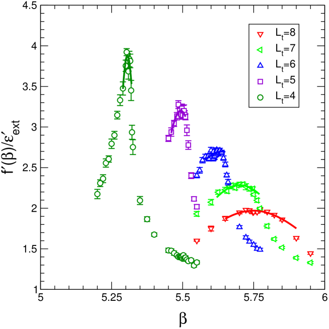
Figure 1: $f^{\prime}$ vs. $\beta$ at fixed external field strength ($n_{\text{ext}}=1$) for $L_{t}=4,5,6,7,8$ and $L_{s}=64$. Solid lines are the fits Eq. (12).

As is well known pure SU(3) gauge system undergoes a deconfinement phase transition by increasing temperature. As a matter of fact, it turns out that the knowledge of $f^{\prime}[\vec{A}^{\mathrm{ext}}]$ at finite temperature can be used to estimate the critical temperature $T_{c}$. To this end it suffices to evaluate $f^{\prime}[\vec{A}^{\mathrm{ext}}]$ as a function of $\beta$ for different lattice temporal sizes $L_{t}$. Indeed we found that $f^{\prime}[\vec{A}^{\mathrm{ext}}]$ displays a peak in the critical region. In Figure 1 we display the peak regions for different values of $L_{t}$. We see clearly that the pseudocritical coupling, which is the value of $\beta$ at the peak, depends on $L_{t}$. In order to determine the pseudocritical couplings $\beta^{*}(L_{t})$ we parameterize $f^{\prime}(\beta,L_{t})$ near the peak as:

$$\frac{f^{\prime}(\beta,L_{t})}{\varepsilon^{\prime}_{\mathrm{ext}}}=\frac{a_{1}(L_{t})}{a_{2}(L_{t})[\beta-\beta^{*}(L_{t})]^{2}+1}\,.$$ (12)

In Eq. (12) we normalize $f^{\prime}$ to $\varepsilon^{\prime}_{\mathrm{ext}}$, the derivative of the classical energy due to the external applied field

$$\varepsilon^{\prime}_{\mathrm{ext}}=\frac{2}{3}\,[1-\cos(\frac{gH}{2})]=\frac{2}{3}\,[1-\cos(\frac{2\pi}{L_{1}}n_{\mathrm{ext}})].$$ (13)

We restrict the region near $\beta^{*}(L_{t})$ until the fits Eq. (12) give a reduced $\chi^{2}/{\text{ d.o.f.}}\sim 1$. Once determined $\beta^{*}(L_{t})$ we estimate the deconfinement temperature as

$$\frac{T_{c}}{\Lambda_{\mathrm{latt}}}=\frac{1}{L_{t}}\frac{1}{f_{SU(3)}(\beta^{*}(L_{t}))}\,,$$ (14)

where

$$f_{SU(N)}(\beta)=\left(\frac{\beta}{2Nb_{0}}\right)^{b_{1}/2b_{0}^{2}}\,\exp\left(-\beta\frac{1}{4Nb_{0}}\right)\,$$ (15)

$N$ being the color number, $b_{0}=(11N)/(48\pi^{2})$, and $b_{1}=(34N^{2})/(3(16\pi^{2})^{2})$.

In order to obtain the continuum limit critical temperature we have to extrapolate $T_{c}/\Lambda_{\mathrm{latt}}$, given by Eq. (14), to the continuum.

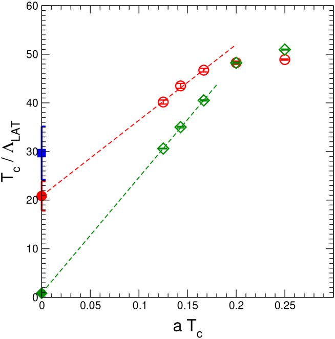
Figure 2: $T_{c}/\Lambda_{\mathrm{latt}}$ versus $aT_{c}$ for two different values of the external field strength ($n_{\text{ext}}=1$ open circles, $n_{\text{ext}}=10$ open diamonds). Full points refer to the continuum extrapolations. Full square is the critical temperature Eq. (16).

In Figure 2 we display $T_{c}/\Lambda_{\mathrm{latt}}$ as a function of $aT_{c}$ for two different values of the chromomagnetic background field. To extract the continuum limit of the critical temperature we follow Ref. [40] and perform a linear extrapolation to the continuum of our data for $T_{c}/\Lambda_{\mathrm{latt}}$. For comparison we also display in Fig. 2 the continuum limit of the critical temperature without background field [40]

$$\frac{T_{c}}{\Lambda_{\mathrm{latt}}}\,=\,29.67\,\pm\,5.47\,.$$ (16)

We see clearly that the continuum limit deconfinement critical temperature does depend on the applied Abelian chromomagnetic field. Therefore we decided to vary the strength of the applied external Abelian chromomagnetic background field to study quantitatively the dependence of $T_{c}$ on $gH$ [41].

To this aim we performed numerical simulations on $64^{3}\times L_{t}$ lattices with $n_{\text{ext}}=1,2,3,5,10$. Since we are measuring a local quantity, such as average plaquette, a low statistics (from 1000 up to 5000 configurations) is required in order to get a good estimate of $f^{\prime}[\vec{A}^{\mathrm{ext}}]$. Statistical errors have been estimated using the jackknife resampling method modified to take into account the statistical correlations between lattice configurations. As a check of possible finite volume effects we also simulated our gauge system on $128\times 64^{2}\times L_{t}$ lattice with $n_{\text{ext}}=3$. Indeed, we found that our numerical data do not display appreciable finite volume effects.

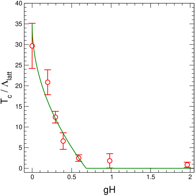
Figure 3: The continuum critical temperature $T_{c}/\Lambda_{\mathrm{latt}}$ versus the external field strength $gH$. Solid line is the fit of Eq. (18) to our data.

Following previous steps we are able to determine the critical temperature as a function of the external chromomagnetic field. In Figure 3 we display our determination of $T_{c}$ for different values of the applied field strength. We see that the critical temperature decreases by increasing the external Abelian chromomagnetic field. If the magnetic length $a_{H}\sim 1/\sqrt{gH}$ is the only relevant scale of the problem, then for dimensional reasons one expects that

$$T_{c}^{2}\,\,\sim\,\,gH\,.$$ (17)

Indeed we try to fit our data with

$$\frac{T_{c}(gH)}{\Lambda_{\text{latt}}}=\frac{T_{c}(0)}{\Lambda_{\text{latt}}}+\alpha\sqrt{gH}\,.$$ (18)

We find a satisfying fit (see Fig. 3) with $\alpha=-42.4\pm 7.4$ and $T_{c}(0)/\Lambda_{\text{latt}}$ that agrees within errors with Eq. (16). Remarkably, we see that there exists a critical field

$$gH_{c}\simeq 0.68$$ (19)

such that $T_{c}=0$ for $gH>gH_{c}$.

Let us conclude by stressing the main results of this paper. We found that there is a critical field $gH_{c}$ such that, for $gH>gH_{c}$, the gauge system is in the deconfined phase. As a consequence, we see that there is an intimate connection between Abelian chromomagnetic fields and color confinement. The existence of a critical chromomagnetic field is not easily understandable within the coherent magnetic monopole condensate picture of the confining vacuum. On the other hand, it could be explained if the vacuum behaves as an ordinary relativistic color superconductor. Thus we have to reconcile two apparently different aspects. From one hand, the confining vacuum does display condensation of both Abelian magnetic monopoles and vortices, on the other hand the relation between the deconfinement temperature and the applied Abelian chromomagnetic field consistent with Eq. (17) suggests that the vacuum behaves as a condensate of a color charged scalar field whose mass is proportional to the inverse of the magnetic length. A natural candidate for such tachyonic color charged scalar field is the famous Nielsen-Olesen unstable mode [42]. The eventual condensation of the Nielsen-Olesen modes makes the vacuum a dynamical color superconductor. However, it should be stressed that, unlike the case of an elementary color charged scalar field, the chromomagnetic condensate cannot be uniform due to gauge invariance of the vacuum. Indeed, as showed [43] by R. P. Feynman (in 2+1 dimensions) gauge invariance of the ground state disorders the system in such a way that there are not long range color correlations. In this way the disordered chromomagnetic condensate should lead to the screening of any external Abelian chromomagnetic charge, thus explaining the condensation of both Abelian chromomagnetic monopoles and vortices.

Another important aspect of this work might be related to astrophysics applications. Indeed, aside from the above considerations, our result implies that it is possible to deconfine quarks and gluons even at low temperature and low density. As a consequence follows the exciting possibility of low density compact quark stars. Obviously, further progress on this matter needs the equation of state appropriate for the description of deconfined quarks and gluons in an Abelian chromomagnetic field.

References

- [1] G. ’t Hooft, High Energy Physics, EPS International Conference, Palermo, 1975.
- [2] S. Mandelstam, Phys. Rept. 23 (1976) 245.
- [3] J. Wosiek and R.W. Haymaker, Phys. Rev. D36 (1987) 3297.
- [4] A. Di Giacomo, M. Maggiore and S. Olejnik, Nucl. Phys. B347 (1990) 441.
- [5] P. Cea and L. Cosmai, Nucl. Phys. Proc. Suppl. 30 (1993) 572.
- [6] V. Singh, D.A. Browne and R.W. Haymaker, Nucl. Phys. Proc. Suppl. 30 (1993) 568, hep-lat/9302010.
- [7] Y. Matsubara, S. Ejiri and T. Suzuki, Nucl. Phys. Proc. Suppl. 34 (1994) 176, hep-lat/9311061.
- [8] G.S. Bali, K. Schilling and C. Schlichter, Phys. Rev. D51 (1995) 5165, hep-lat/9409005.
- [9] P. Cea and L. Cosmai, Phys. Lett. B349 (1995) 343, hep-lat/9404017.
- [10] P. Cea and L. Cosmai, Phys. Rev. D52 (1995) 5152, hep-lat/9504008.
- [11] A. Di Giacomo, Nucl. Phys. Proc. Suppl. 47 (1996) 136, hep-lat/9509036.
- [12] J.D. Stack and R.J. Wensley, Nucl. Phys. B371 (1992) 597.
- [13] H. Shiba and T. Suzuki, Phys. Lett. B351 (1995) 519, hep-lat/9408004.
- [14] N. Arasaki et al., Phys. Lett. B395 (1997) 275, hep-lat/9608129.
- [15] N. Nakamura et al., Nucl. Phys. Proc. Suppl. 53 (1997) 512, hep-lat/9608004.
- [16] M.N. Chernodub, M.I. Polikarpov and A.I. Veselov, Phys. Lett. B399 (1997) 267, hep-lat/9610007.
- [17] J. Jersak, T. Neuhaus and H. Pfeiffer, Phys. Rev. D60 (1999) 054502, hep-lat/9903034.
- [18] A. Di Giacomo et al., Phys. Rev. D61 (2000) 034503, hep-lat/9906024.
- [19] A. Di Giacomo et al., Phys. Rev. D61 (2000) 034504, hep-lat/9906025.
- [20] P. Cea and L. Cosmai, Nucl. Phys. Proc. Suppl. 83 (2000) 428, hep-lat/9909056.
- [21] C. Hoelbling, C. Rebbi and V.A. Rubakov, Phys. Rev. D63 (2001) 034506, hep-lat/0003010.
- [22] P. Cea and L. Cosmai, Phys. Rev. D62 (2000) 094510, hep-lat/0006007.
- [23] J.M. Carmona et al., (2001), hep-lat/0103005.
- [24] P. Cea, L. Cosmai and A.D. Polosa, Phys. Lett. B392 (1997) 177, hep-lat/9601010.
- [25] P. Cea and L. Cosmai, Phys. Rev. D60 (1999) 094506, hep-lat/9903005.
- [26] M. Lüscher et al., Nucl. Phys. B384 (1992) 168, hep-lat/9207009.
- [27] M. Lüscher and P. Weisz, Nucl. Phys. B452 (1995) 213, hep-lat/9504006.
- [28] P.H. Damgaard and U.M. Heller, Phys. Rev. Lett. 60 (1988) 1246.
- [29] P. Cea and L. Cosmai, Phys. Rev. D43 (1991) 620.
- [30] P. Cea and L. Cosmai, Phys. Lett. B264 (1991) 415.
- [31] A.R. Levi and J. Polonyi, Phys. Lett. B357 (1995) 186, hep-lat/9505007.
- [32] M. Ogilvie, Nucl. Phys. Proc. Suppl. 63 (1998) 430, hep-lat/9709127.
- [33] M.N. Chernodub, E.M. Ilgenfritz and A. Schiller, Phys. Rev. D64 (2001) 114502, hep-lat/0106021.
- [34] J. Ambjorn et al., Phys. Lett. B225 (1989) 153.
- [35] J. Ambjorn, V.K. Mikryushkin and A.M. Zadorozhnyi, Phys. Lett. B245 (1990) 575.
- [36] K. Kajantie et al., Nucl. Phys. B544 (1999) 357, hep-lat/9809004.
- [37] D.J. Gross, R.D. Pisarski and L.G. Yaffe, Rev. Mod. Phys. 53 (1981) 43.
- [38] P. Cea and L. Cosmai, (2001), hep-lat/0101017.
- [39] P. Cea and L. Cosmai, JHEP 11 (2001) 064.
- [40] J. Fingberg, U. Heller and F. Karsch, Nucl. Phys. B392 (1993) 493, hep-lat/9208012.
- [41] P. Cea and L. Cosmai, Nucl. Phys. Proc. Suppl. 106 (2002) 613, hep-lat/0109030.
- [42] N.K. Nielsen and P. Olesen, Nucl. Phys. B144 (1978) 376.
- [43] R.P. Feynman, Nucl. Phys. B188 (1981) 479.