Scaling Laws and Effective Dimension in Lattice
$SU(2)$ Yang-Mills Theory
with a Compactified Extra Dimension

Abstract

Monte Carlo simulations are performed in a five-dimensional lattice $SU(2)$ Yang-Mills theory with a compactified extra dimension, and scaling laws are studied. Our simulations indicate that as the compactification radius $R$ decreases, the confining phase spreads more and more to the weak coupling regime, and the effective dimension of the theory changes gradually from five to four. Our simulations also indicate that the limit $a_{4}\to 0$ with $R/a_{4}$ kept fixed exists both in the confining and deconfining phases if $R/a_{4}$ is small enough, where $a_{4}$ is the lattice spacing in the four-dimensional direction. We argue that the color degrees of freedom in QCD are confined only for $R<R_{\rm max}$, where a rough estimate shows that $1/R_{\rm max}$ lies in the TeV range. Comments on deconstructing extra dimensions are given.

I Introduction

Since Kaluza and Klein [1] found that the electromagnetic and gravitational forces can be unified by introducing the fifth dimension, their idea has attracted attention for many decades. Recently, there have been a lot of renewed interests in field theories with extra dimensions, in which the length scale of the extra dimensions can be so large that they could be experimentally observed [2, 3, 4]. It is assumed there that for distances larger than the compactification size, the massive Kaluza-Klein excitations decouple so that these theories behave as a four-dimensional continuum theory at low energies. Since, however, Yang-Mills theories in more than four dimensions are nonrenormalizable, it is not at all clear that the infinite tower of the Kaluza-Klein excitations decouple even if each massive excitation is suppressed: A naive expectation of their contribution would be $\infty\cdot 0$.

At four dimensions, the color degrees of freedom are confined even for a weak gauge coupling. How can a confining four-dimensional Yang-Mills theory emerge from a higher-dimensional Yang-Mills theory which is deconfining in the weak coupling regime [5, 6, 7] ? Although the assumption on the decoupling of the Kaluza-Klein excitations sounds physically correct, it is by no means trivial that they nonperturbatively decouple in such a way that the color confinement takes place even at a weak gauge coupling. Recently, we [8] have started to address related problems in a concrete example, namely the pure lattice $SU(2)$ Yang-Mills theory in five dimensions with one dimension compactified on a circle. We have observed [8] that the compactification changes the nature of the phase transition, and that a second order phase transition, which does not exist in the uncompactified case, occurs, thus confirming the long-standing expectation of Lang, Pilch and Skagerstam[6]. For the first time, we [8] have computed the lattice $\beta$-function in a Yang-Mills theory in more than four dimensions, and have verified nonperturbatively the power-law running of the gauge coupling constant [4, 9, 10, 11].

In this paper we would like to extend the analyses of [8]. We first observe that if the compactification radius becomes smaller and smaller, the confining phase spreads more and more to the weak coupling regime. At the same time we compute the effective dimension [12, 13], and see that the theory behaves more and more as a four-dimensional Yang-Mills theory. Based on this result, we argue that the color degrees of freedom in QCD are confined only for $R<R_{\rm max}$. Our rough estimate yields that $1/R_{\rm max}$ lies in the TeV range.

Our calculations of the potential between two static quarks separated in the four-dimensional subspace show that the deconfining phase is a Coulomb phase. We then discuss the nature of the transition from the deconfining phase to the confining phase for fixed values of $R/a_{4}$, where $a_{4}$ is the lattice spacing in the four-dimensional direction. We confirm that if $R/a_{4}$ is small enough, it is consistent with a second order transition . Combined with the result of [8], we therefore come to the conclusion that as we decrease the value of $R\Lambda$, the first order transition for large values of $R\Lambda$ changes to a cross over transition, and finally becomes of second order.

We give some nonperturbative comments on deconstructing extra dimensions [14] in Conclusion.

II Effective dimension

In order to take into account the compactification effects in this theory, it is crucial to use anisotropic lattices [15] which has different lattice spacings, $a_{4}$ and $a_{5}$, in the four-dimensional directions and in the fifth direction. For definiteness we employ the Wilson action for pure $SU(2)$ lattice gauge theory

$$S = \frac{\beta}{\gamma}~{}\sum_{P_{4}}~{}[~{}1-\frac{1}{2}~{}\mbox{Re Tr}~{}U_{P_{4}}~{}]+\beta\gamma~{}\sum_{P_{5}}~{}[~{}1-\frac{1}{2}~{}\mbox{Re Tr}~{}U_{P_{5}}~{}]~{},$$ (1)

where $U_{P_{4}}$ denote plaquette variables in the four-dimensional sublattice, and $U_{P_{5}}$ are those which are extended in the fifth dimension. The gauge coupling constant $g_{5}$ has the dimension of $\sqrt{a_{4}}$, which is related to $\beta$ by

$$a_{4}g_{5}^{-2}=\beta/4$$ (2)

at the tree level. Periodic boundary conditions are imposed in all directions, and we use the lattice size of the form $N_{4}^{4}\times N_{5}$ (we mostly use $N_{4}=12$ and $N_{5}=4$). The compactification radius is defined as $R=a_{5}N_{5}/2\pi$ if $N_{4}a_{4}>N_{5}a_{5}$ is satisfied, and the correlation-anisotropy parameter is defined as $\xi=a_{4}/a_{5}$. The tree level relation $\gamma=\xi$ will be modified at the quantum level [15], and throughout this paper we assume that the $\xi-\gamma$ relation obtained in [8] is satisfied both in the confining and deconfining phases. Simulations are performed for

$$\gamma=3.6,4.0,4.6,5.0~{},$$ (3)

which is equivalent to [8]

$$\frac{2\pi R}{a_{4}} = \frac{N_{5}a_{5}}{a_{4}}=\frac{4}{\xi}\approx 0.72,0.64,0.55,0.50~{},$$ (4)

where we have used $N_{5}=4$ above. We have chosen this range of $2\pi R/a_{4}$, because we expect from the previous calculations [8] that the limit $2\pi R/a_{4}\to 0$ may exist and we observe some scaling behavior.

To define the physical scale in the confining phase, we use the string tension $\sigma$ between two static quarks that are separated in the four-dimensional subspace. Since the string tension is a physical quantity, the lattice string tension $\sigma_{L}$ should behave like $a_{4}^{2}$ as $a_{4}\to 0$, where $a_{4}$ can be related by the $\beta$ function to the dimensionless bare gauge coupling

$$g^{2} = \frac{8\pi}{\beta}=\Lambda g_{5}^{2}~{},$$ (5)

where we have identified $\Lambda$ with $2\pi/a_{4}$ because $4\times(\pi/a_{4})^{2}=(2\pi/a_{4})^{2}$. Since we expect that the massive Kaluza-Klein excitations decouple increasingly as $2\pi R/a_{4}$ decreases, the lattice $\beta$ function $\beta_{L}$ cannot assume a purely five- or four-dimensional form. Instead, we expect a continuous change of its form. This is quantitatively expressed by the so-called effective dimension $D_{\rm eff}$ which is a function of $2\pi R/a_{4}$ [13]. So, we assume that $\beta_{L}$ can be written as

$$\beta_{L} = -a_{4}\frac{dg^{2}}{da_{4}}=[~{}D_{\rm eff}(2\pi R/a_{4})-4~{}]~{}g^{2}-\frac{2b}{16\pi^{2}}g^{4}~{},$$ (6)

where $b=22/3-2/3=20/3$. Therefore, the evolution equation of $g^{2}$ can be easily integrated in the case that $2\pi R/a_{4}$ is kept fixed while $a_{4}$ changes. We obtain for this case

$$\sqrt{\sigma_{L}} \sim a_{4}\sim\left(\frac{2b}{16\pi^{2}}\frac{1}{D_{\rm eff}-4}-\frac{\beta}{8\pi}\right)^{1/(D_{\rm eff}-4)}~{}.$$ (7)

It is important to notice that as $D_{\rm eff}\to 4$, we obtain the logarithmic form

$$g^{-2} = \beta/8\pi=(2b/16\pi^{2})\ln a_{4}+const.$$ (8)

That is, if we can show that the effective dimension $D_{\rm eff}$ in the confining phase varies from $5$ to $4$ as $2\pi R/a_{4}$ decreases from a larger value to a smaller value, we show the continuous decoupling of the Kaluza-Klein excitations, and the confining phase spreads more and more to the weak coupling regime as $R$ decreases.

III Confining phase

Now we come to the results of our Monte Carlo simulations on a $12^{4}\times 4$ lattice. We use the Creutz ratio $\chi(I,J)$ obtained from the rectangular Wilson loops $W(I,J)$ with lengths of $I$ and $J$ in the four-dimensional subspace. We assume that the Creutz ratio takes the form

$$\chi(I,J)=\chi_{0}-\chi_{1}\left(\frac{1}{I(I-1)}+\frac{1}{J(J-1)}\right)+\chi_{2}\left(\frac{1}{I(I-1)J(J-1)}\right)~{},$$ (9)

and we identity $\chi_{0}$ with the lattice string tension $\sigma_{L}$. We have generated 2500 configurations for each simulation point after thermalization, and the Wilson loops are measured every 5 configurations for the calculation of a Creutz ratio. Errors are estimated by the jackknife method. The filled symbols in Fig. 1 are the result obtained from the Monte Carlo simulations with $\gamma=5.0$, where the vertical axis stands for $\sqrt{\chi_{0}}=\sqrt{\sigma_{L}}$ and the horizontal axis stands for $\beta$. We have also calculated $\sigma_{L}$ from the static potential to make it sure that $\sigma_{L}$ obtained from the Creutz ratios is reliable . The static potential we have assumed has the form

$$V(X)=C_{0}-C_{1}\frac{1}{X}+C_{2}\left(\frac{1}{X}-\left[\frac{1}{X}\right]\right)+C_{3}X~{},$$ (10)

where $[1/X]$ is the three-dimensional Coulomb potential on a lattice, and is given by

$$\left[\frac{1}{X}\right]=4\pi\int_{-\pi}^{\pi}\frac{d^{3}p}{(2\pi)^{3}}\frac{\exp\{i\sum_{i}X_{i}\sin(p_{i}/2)\}}{\sum_{i=1}^{4}\sin^{2}(p_{i}/2)}~{}.$$ (11)

The open symbols in Fig. 1 correspond to the result obtained from the static potential. Comparing two results in Fig. 1 we see that the lattice string tensions obtained from the Creutz ratios agree with those obtained from the static potential. We have made the same comparison for different values of $\gamma$, and found the same result. So, in the following analyses we use only the lattice string tensions from the Creutz ratio, because we have more data for this case and we do not want to mix data obtained by two different methods.

We see from Fig. 1 that above $\beta\mathrel{\mathchoice{\vbox{\offinterlineskip\halign{$\m@th\displaystyle\hfil#\hfil$\cr>\crcr\sim\crcr} }}{\vbox{\offinterlineskip\halign{$\m@th\textstyle\hfil#\hfil$\cr>\crcr\sim\crcr} }}{\vbox{\offinterlineskip\halign{$\m@th\scriptstyle\hfil#\hfil$\cr>\crcr\sim\crcr} }}{\vbox{\offinterlineskip\halign{$\m@th\scriptscriptstyle\hfil#\hfil$\cr>\crcr\sim\crcr} }}}3.0$ the square root of the lattice string tension $\sqrt{\sigma_{L}}$ decreases first linearly until $\beta\sim 3.3$, and then its slope becomes milder. The tail for large $\beta$ is certainly due to the finite lattice size effects, but the change from the linear decrease of $\sqrt{\sigma_{L}}$ to a milder one around $\beta\sim 3.3$ may indicate that the theoretical expectation (7) is correct. Although it is in principle possible to check by increasing the lattice size how much finite lattice size effects may be contained in the tail of $\sqrt{\sigma_{L}}$, it is impossible to do this at the moment because of the limitation of the computing facility given to us. Below we sketch how we confirm Eq. (7) and compute $D_{\rm eff}$.

The effective dimension can be obtained by fitting the function (7) to the data. To this end, we first choose four neighboring data points that lie around the middle of the data set for a given $\gamma$, and using these points, we fit the function (7) to obtain the effective dimension. (In the case for $\gamma=5.0$ for instance, we use the data points at $\beta=3.20,3.22,3.24$ and $3.26$.) Then we increase the number of the data points, to be used, by two by including the next neighboring data point in both sides. In doing so, we obtain the effective dimension and also $\chi^{2}/\mbox{DOF}$ as a function of the number $n$ of the data points that are used for a fit. We repeat the same analysis for the different values of $2\pi R/a_{4}$ given in (4). The results are shown in Fig. 2, 3 and in Table I. In Fig. 3, the vertical axis stand for $(D_{\rm eff}-4)^{-1}$ and the error bar is computed from $\chi^{2}/\mbox{DOF}$. We see that as $n$ increases, the error bar decreases and the central values converge. The results are summarized in Table I, and we see that the effective dimension $D_{\rm eff}$ decreases gradually from $4.7057(55)$ to $4.5230(82)$ as $\gamma$ increases from $3.6$ to $5.0$, which means, as $2\pi R/a_{4}$ decreases from $0.72$ to $0.5$ (see (4)).

The $\beta^{*}$ in Table I is the value at which $\sigma_{L}$ and hence $a_{4}$ should vanish if the theoretical assumption (7) is correct and extrapolated for larger values of $\beta$ (see also Fig. 2). We emphasize that our results indicate that the limit $a_{4}\to 0$ with $R/a_{4}$ kept fixed exists in the confining phase at finite $\beta$.

IV The maximal radius

The same analysis in the real QCD in section III would constrain the size of the compactification radius in QCD, which we would like to estimate without detailed calculations. To see that there exists the maximal radius for color confinement in the four-dimensional subspace, we recall the results obtained in the previous section and those from the next section:

$$g^{2}\mathrel{\mathchoice{\vbox{\offinterlineskip\halign{$\m@th\displaystyle\hfil#\hfil$\cr>\crcr\sim\crcr} }}{\vbox{\offinterlineskip\halign{$\m@th\textstyle\hfil#\hfil$\cr>\crcr\sim\crcr} }}{\vbox{\offinterlineskip\halign{$\m@th\scriptstyle\hfil#\hfil$\cr>\crcr\sim\crcr} }}{\vbox{\offinterlineskip\halign{$\m@th\scriptscriptstyle\hfil#\hfil$\cr>\crcr\sim\crcr} }}}(\mathrel{\mathchoice{\vbox{\offinterlineskip\halign{$\m@th\displaystyle\hfil#\hfil$\cr<\crcr\sim\crcr} }}{\vbox{\offinterlineskip\halign{$\m@th\textstyle\hfil#\hfil$\cr<\crcr\sim\crcr} }}{\vbox{\offinterlineskip\halign{$\m@th\scriptstyle\hfil#\hfil$\cr<\crcr\sim\crcr} }}{\vbox{\offinterlineskip\halign{$\m@th\scriptscriptstyle\hfil#\hfil$\cr<\crcr\sim\crcr} }}})(D_{\rm eff}-4)(16\pi^{2}/2b)~{}~{}\mbox{for the (de)confining phase}~{}.$$ (28)

Therefore, for a given value of $D_{\rm eff}$, there should exist the smallest value of $g^{2}$ for color confinement to occur, which is $\sim(D_{\rm eff}-4)(16\pi^{2}/2b)$. The question is how $g^{2}$ can be related to the gauge coupling $g_{\rm kk}^{2}$ of the Kaluza-Klein theory, the four-dimensional theory with the Kaluza-Klein tower. At the tree level, it is $g^{2}_{\rm kk}=g^{2}(2\pi R\Lambda)^{-1}$, but in higher orders this relation will receive quantum corrections, where we have used $\Lambda^{2}=(\pi/a_{4})^{2}\times 4$. To answer the question, we first assume that $D_{\rm eff}(R\Lambda)\to 4(5)$ as $R\Lambda\to 0(\infty)$, and we consider a redefinition of $g^{2}$ according to [12, 13]

$$g^{2}_{\rm kk} = \eta^{-1}(R\Lambda)g^{2}~{},~{}\eta(t)=\exp\int_{0}^{t}\frac{dt^{\prime}}{t^{\prime}}(D_{\rm eff}(t^{\prime})-4)~{}.$$ (29)

Note that the $\beta$ function of $g^{2}_{\rm kk}$ becomes

$$\beta_{\rm kk} = -(2b/16\pi^{2})\eta(R\Lambda)g^{4}_{\rm kk}~{}.$$ (30)

Since the function $\eta(R\Lambda)$ becomes proportional to $R\Lambda$ as $R\Lambda\to\infty$ , the new gauge coupling describes the power-law behavior [4, 9, 10, 11]. Furthermore, we see from (29) that $g^{2}_{\rm kk}$ approaches $g^{2}$ as $R\Lambda$ approaches $0$. Recalling now the assumption that $D_{\rm eff}$ approaches $4$ as $R\Lambda$ approaches $0$ and Eq. (8), we see that the renormalization group flow of the new gauge coupling $g^{2}_{\rm kk}$ for small $R\Lambda$ takes exactly the same form as the one for the effective, four-dimensional theory without the Kaluza-Klein tower. Therefore, we assume that $g_{\rm kk}^{2}$ is the gauge coupling of the four-dimensional theory with the Kaluza-Klein tower.

Now, suppose that QCD results from a five-dimensional QCD. As we have argued above, $g^{2}$ becomes $g_{\rm kk}^{2}$ at low energies, and we then identify $2\pi/a_{4}$ with the physical scale $\Lambda$ of the effective theory, rather than with the ultraviolet cutoff. Since $g^{2}(M_{Z})/4\pi\simeq 0.12$ in QCD and $b=7$, the constraint (28) can be converted to that of the effective dimension, i.e., $D_{\rm eff}(RM_{Z})\mathrel{\mathchoice{\vbox{\offinterlineskip\halign{$\m@th\displaystyle\hfil#\hfil$\cr<\crcr\sim\crcr} }}{\vbox{\offinterlineskip\halign{$\m@th\textstyle\hfil#\hfil$\cr<\crcr\sim\crcr} }}{\vbox{\offinterlineskip\halign{$\m@th\scriptstyle\hfil#\hfil$\cr<\crcr\sim\crcr} }}{\vbox{\offinterlineskip\halign{$\m@th\scriptscriptstyle\hfil#\hfil$\cr<\crcr\sim\crcr} }}}4.13$. Therefore, if we know the function $D_{\rm eff}(t)$ exactly, we can calculate the range of $t$ for which the inequality (28) is satisfied. From the result given in Table I we find that the effective dimension as a function of $t$ can be written as $D_{\rm eff}(t)\simeq 4+t$. Assuming that this function can be used even for small $t$, we then obtain $R\Lambda\mathrel{\mathchoice{\vbox{\offinterlineskip\halign{$\m@th\displaystyle\hfil#\hfil$\cr<\crcr\sim\crcr} }}{\vbox{\offinterlineskip\halign{$\m@th\textstyle\hfil#\hfil$\cr<\crcr\sim\crcr} }}{\vbox{\offinterlineskip\halign{$\m@th\scriptstyle\hfil#\hfil$\cr<\crcr\sim\crcr} }}{\vbox{\offinterlineskip\halign{$\m@th\scriptscriptstyle\hfil#\hfil$\cr<\crcr\sim\crcr} }}}0.13$, which implies that

$$1/R\mathrel{\mathchoice{\vbox{\offinterlineskip\halign{$\m@th\displaystyle\hfil#\hfil$\cr>\crcr\sim\crcr} }}{\vbox{\offinterlineskip\halign{$\m@th\textstyle\hfil#\hfil$\cr>\crcr\sim\crcr} }}{\vbox{\offinterlineskip\halign{$\m@th\scriptstyle\hfil#\hfil$\cr>\crcr\sim\crcr} }}{\vbox{\offinterlineskip\halign{$\m@th\scriptscriptstyle\hfil#\hfil$\cr>\crcr\sim\crcr} }}}O(1)\mbox{ TeV}$$ (39)

should be satisfied for the color degrees of freedom in QCD to be confined. The number above should not be taken very seriously, because our estimate is based on many theoretical assumptions, which can be justified if we perform simulations on five-dimensional, compactified $SU(3)$ lattice gauge theory. The crucial point is that there exists the maximal radius.

V Coulomb phase

The confining phase shrinks as $R$ decreases, which we have already seen above. Next we would like to show that the deconfining phase is a Coulomb phase. To begin with, we consider the Wilson loop $W(\vec{x},t)$ at the tree level in continuum perturbation theory. The static potential can be obtained by

$$V(x) = \lim_{t\to\infty}(\ln W(\vec{x},t))/t=-\frac{3}{4}g_{5}^{2}~{}\frac{1}{2\pi R}\frac{1}{4\pi x}\coth\left(\frac{x}{2R}\right)$$ (40)

$$= -\frac{3}{4}g_{5}^{2}~{}\left\{\begin{array}[]{@{\,}ll}\frac{\displaystyle 1}{\displaystyle 4\pi^{2}x^{2}}&\left(\frac{\displaystyle x}{\displaystyle 2R}\ll 1\right)\\ &\\ \frac{\displaystyle 1}{\displaystyle 2\pi R}\frac{\displaystyle 1}{\displaystyle 4\pi x}&\left(\frac{\displaystyle x}{\displaystyle 2R}\gg 1\right)\\ \end{array}~{}.\right.$$ (44)

We have the usual Coulomb potential for $x/2R\gg 1$, and we see that the dimensionless gauge coupling $\hat{g}$, normalized for the four-dimensional Yang-Mills theory at the tree level, is given by $\hat{g}=g_{5}/\sqrt{2\pi R}$ as well known [3, 4]. The corresponding expression on a lattice is

$$V_{L}(X) = \lim_{T\to\infty}\ln W(X,T)/W(X,T+1)~{},$$ (45)

where $W(X,T)$ is a lattice Wilson loop. The lattice distances $X$ and $T$ are made dimensionless by dividing by $a_{4}$. We are interested in the potential between two static quarks that are separated in four dimensions, and therefore, $X$ and $T$ are supposed to be in the four-dimensional sublattice. Since in the actual calculations we cannot take the limit $T\to\infty$, we consider also off-axis loops and use the standard smearing techniques [16] to improve the convergence of approximants with increasing $T$. Our smearing procedure consists of iteratively replacing each spatial (three-dimensional) link by the sum of itself and the neighboring four spatial staples with a weight parameter $\epsilon$,

$$U_{i}(x,y) \to U^{\prime}_{i}(x,y)={\cal P}_{SU(2)}\left(U_{i}(x,y)+\epsilon\sum_{j(\neq i)=1}^{3}F_{ij}(x,y)\right)$$ (46)

$$F_{ij}(x,y) = U_{j}(x,y)U_{i}(x+\hat{j},y)U^{\dagger}_{j}(x+\hat{i},y)+U^{\dagger}_{j}(x-\hat{i},y)U_{i}(x-\hat{i},y)U_{j}(x-\hat{i}+\hat{j},y)~{},$$ (47)

where ${\cal P}_{SU(2)}$ denotes a projection operator, back onto the $SU(2)$ manifold.

We have generated 10000 configurations for each simulation point after thermalization, and the smeared Wilson loops are measured every 100 configurations for the calculation of the static potential. We iterate Eq.(46) 60 times with $\epsilon=0.1$ in the case of the confining phase, 100 times with $\epsilon=0.2$ in the case of the Coulomb phase. In Fig. 4 we show the result (filled symbols) for the lattice potential $V_{L}(X)$ as a function of $X$ at $\beta=5.0$ and $\gamma=5.0$ (which is equivalent to $2\pi R/a_{4}=0.5)$. The condition $x/2R\gg 1$ to obtain a $1/X$ potential becomes $X\gg 1/2\pi$ in this case, and we assume that the lattice potential $V_{L}(X)$ takes the form

$$V_{L}(X)=C_{0}-C_{1}\frac{1}{X}+C_{2}\left(\frac{1}{X}-\left[\frac{1}{X}\right]\right)~{},$$ (48)

where is $[1/X]$ (the three-dimensional Coulomb potential on a lattice is given in (11). The first term of (48) is the unphysical self energy, the second term is a rotationally invariant part of the Coulomb potential, and third term is the most dominant part of its breaking. From a $\chi^{2}$ fit we find that $C_{0}=0.3230(14),C_{1}=0.1086(30),C_{2}=0.0776(27)$. The fitted lattice potential with the $C_{2}$ term in (48) suppressed, i.e.

$$V(X)=C_{0}-C_{1}\frac{1}{X}~{},$$ (49)

is the dotted curve in Fig. 4, while the open symbols stand for the rotationally invariant data points. We see that the data justify the assumption that the deconfining phase is a Coulomb phase.

VI Nature of the phase transition

As the next task we consider the nature of the transition from the confining phase to the Coulomb phase. In the confining phase our data indicate that the limit $a_{4}\to 0$ with $R/a_{4}$ kept fixed exists at finite $\beta$. If we can show that $a_{4}$ also vanishes at the same value of $\beta$ in the Coulomb phase, the transition from the confining phase to the Coulomb phase is of second order.

To this end, we have to define the scale in the Coulomb phase. In the naive continuum theory there are two dimensional quantities, the gauge coupling $g_{5}$ and the compactification radius $R$. Therefore, we assume that $R$ and the low-energy value of $g_{5}$ are independent physical quantities at the quantum level, too. We then consider the limit $a_{4}\to 0$ with $2\pi R/a_{4}$ kept fixed, which is the same limiting process we have considered in the confining phase. In this limit, the quantity $g_{5}^{2}/2\pi R$ (the coefficient $C_{1}$ of the tree-level Coulomb potential (48)) has to diverge because $R\to 0$ while $g_{5}$ should remain finite by assumption. So naively one expects the scaling law $C_{1}^{-1}\sim R\sim a_{4}\sim(\beta-\beta^{*})$, where $\beta^{*}$ is the critical value of $\beta$ at which $\sigma_{L}^{1/2}\sim a_{4}$ vanishes. In Fig. 5 we plot $C_{1}^{-1}$ versus $\beta$ for different values of $\gamma$ (or $2\pi R/a_{4}$ of (4)). We see that $C_{1}^{-1}$ linearly decreases, and make therefore a theoretical ansatz for the scaling law:

$$C_{1}^{-1} = D_{0}-D_{1}\beta~{}.$$ (50)

For $\gamma=4.6$, for instance, a $\chi^{2}$ fit yields that $D_{0}=9.16(36)$ and $D_{1}=3.894(77)$. If the tree-level equation (44) would be correct at the quantum level, too, then it would mean that $a_{4}$ vanishes at $\beta=D_{0}/D_{1}=2.35(14)$ in the deconfining phase. This would contradict the assumption that in the confining phase the lattice spacing $a_{4}$ approaches zero as $\beta$ approaches $\sim 3.7$ for $\gamma=4.6$ (see Table I). This does not necessarily mean that the transition from the deconfining phase to the confining one is a first order transition or a cross over transition. It may be well possible that the tree-level form (44) receives quantum corrections in such a way that the transition is indeed of second order. Therefore, we consider possible quantum corrections to $C_{1}^{-1}$ which are consistent with the scaling law in Fig. 5 and the value of $\beta^{*}$ in the confining phase (given Table I). Since $C_{1}^{-1}$ being dimensionless can depend only on the combination $R/g^{2}_{5}$, the correction can only be a constant, i.e.,

$$C_{1}^{-1} \sim 2\pi R/g^{2}_{5}+\alpha~{}\mbox{or}~{}~{}C_{1}\sim\frac{g^{2}_{5}}{2\pi R+\alpha g_{5}^{2}}~{}.$$ (51)

In Table III we give the results of the fits, from which we find that the ansatz for the nonperturbative quantum correction to the coefficient of the Coulomb potential (48) is consistent with our data, and we conclude that

$$\alpha = 5.1\pm 0.7~{},$$ (52)

where we have not included the data for $\gamma=5.0$ in (52), because the error for this case is very large compared with others. This indicates that the assumption that the transition from the confining to the deconfining phase is a second order transition is consistent with the data. Note that the transition for small values of $\gamma$, or large values of $R\Lambda$, is of first order [6, 8]. We expect that the first order transition for large values of $R\Lambda$ changes to a cross over transition, and finally to the second order transition as we decrease the value of $R\Lambda$

The nonperturbative correction (51) means that the tree level relation $\hat{g}^{2}=g_{5}^{2}/2\pi R$ should be modified to

$$\hat{g}^{2} = \frac{g_{5}^{2}}{2\pi R}(1+\alpha\frac{g_{5}^{2}}{2\pi R})^{-1}~{}.$$ (53)

Since $\alpha$ is large, the correction is not small. The Coulomb phase may be of phenomenological importance, because the color degrees of freedom do not need to be always confined. The $SU(2)$ part of the standard model, for instance, could result from a higher-dimensional Yang-Mills theory in the Coulomb phase. Then the equation like Eq. (53) defines the matching condition.

VII Conclusion

In this paper we have performed Monte Carlo simulations in a five-dimensional lattice $SU(2)$ Yang-Mills theory, where we have compactified one extra dimension. We have found that as the compactification radius $R$ decreases, the confining phase spreads more and more to the weak coupling regime, and the effective dimension of the theory gradually changes from five to four. Our data indicate that for fixed $R/a_{4}$ the transition from the deconfining phase to the Coulomb phase is of second order if $R/a_{4}$ is small enough.

Assuming that the real four-dimensional QCD results from the five-dimensional QCD at low-energies, we have estimated the largest compactification radius $R_{\rm max}$ so that the color degrees of freedom in four dimensions are confined. Our estimate (39) should be understood as the first try, because our calculations are based on many theoretical assumptions, which can be justified if we perform simulations on five-dimensional, compactified $SU(3)$ lattice gauge theory. The striking fact is that there exists the maximal radius, and this may give an important phenomenological constraint for model building based on the Kaluza-Klein theories.

The parameter regime we have considered in the present work corresponds to the regime in which the Kaluza-Klein idea is expected to be realized: At short distances we have the five-dimensional rotational invariance, and at long distances, the Kaluza-Klein excitations decouple so that the low-energy effective theory is a four-dimensional Yang-Mills theory. We found no indication that would contradict this picture. Moreover, the compactified five-dimensional theory, which is perturbatively nonrenormalizable, has the predictive power (unless examined at very short distances), which we conclude from the scaling laws we observe. (The readers are also invited to [17].)

The parameter regime that corresponds to deconstructing extra dimensions [14] is not the same as above [18]; two phases are nonperturbatively separated [8, 18]. In the phase for the conventional Kaluza-Klein theory, the vacuum expectation value of the Ployakov loop (that extends into the fifth dimension) is nonzero [8], while it vanishes [18] in the phase for deconstructing extra dimensions. (The phase for deconstructing extra dimensions is the one in which the layer structure in five-dimensional gauge theories can be realized [19]). Although it is not at al clear that the five-dimensional rotational invariance at short distances is recovered, it looks at the moment as if two different confining four-dimensional Yang-Mills theories could result from two different phases (one from each) of a five-dimensional theory. The difference is purely nonperturbative. It will be very exiting to investigate this difference more in detail, especially, in supersymmetric cases, where one has already analytic results, and it is shown that the five-dimensional Lorentz invariance is recovered [20].

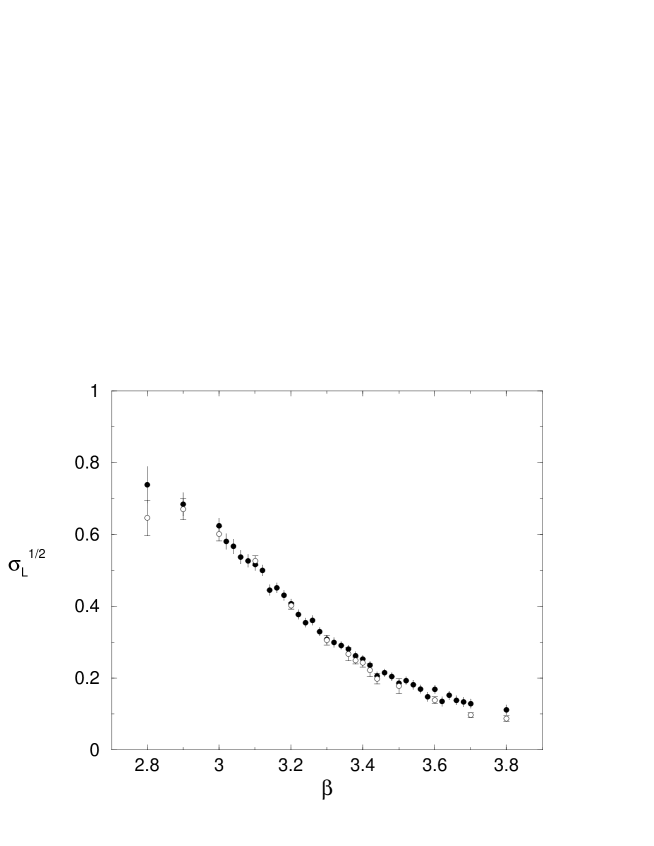
FIG. 1.: $\sqrt{\chi_{0}}=\sqrt{\sigma_{L}}$ versus $\beta$ at $\gamma=5.0$. The filled symbols are obtained from the Creutz ratio (9) and the open ones are obtained from the static potential (10).

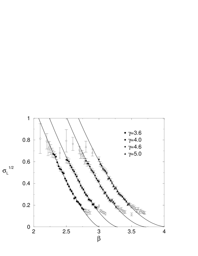
FIG. 2.: The scaling behavior of $\sigma_{L}^{1/2}$ for different values of $\gamma$. The solid lines are drawn by using (7), where $D_{\rm eff}$ is taken from Table I. The data with a filled symbol are used for the fit.

FIG. 3.: The effective dimension as a function of the number $n$ of the data points that are used for a fit. We increase $n$ starting from four till the value of $(D_{\rm eff}-4)^{-1}$ becomes stabilized.

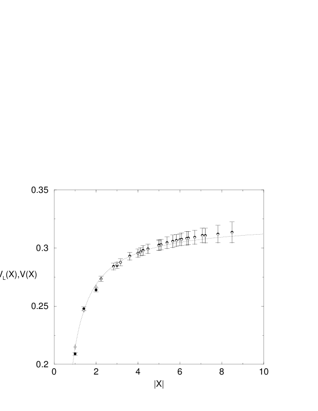
FIG. 4.: The Coulomb potential (45). The filled symbols are the raw data points, and the dotted line is $V(X)$ of Eq. (49) with $C_{0}=0.3230(14)$ and $C_{1}=0.1086(30)$. The open symbols stand for the rotationally invariant data points.

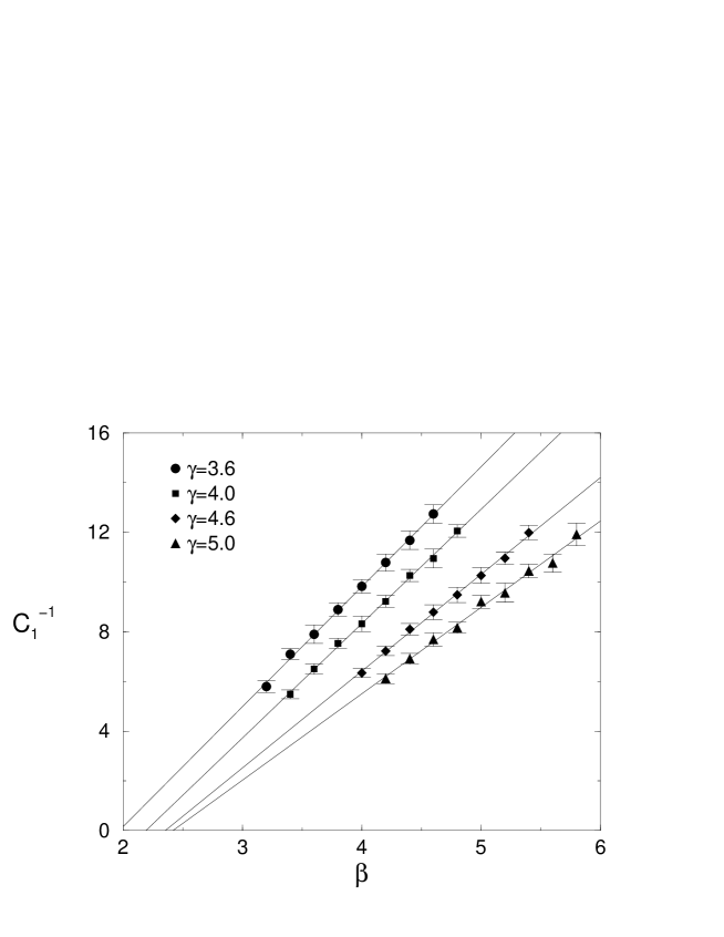
FIG. 5.: $C_{1}^{-1}$ versus $\beta$ for different $\gamma$’s, where $C_{1}^{-1}$ is defined in Eq. (48). The graph shows the scaling behavior in the Coulomb phase. The lines correspond to the linear function (50), where $D_{0}$ and $D_{1}$ are given in Table II.

TABLE I.: Effective dimension for different values of $\gamma$. ($\Lambda=2\pi/a_{4}$)

$\gamma$	$R\Lambda$	$D_{eff}$	$(\beta_{\mbox{min}}:\beta_{\mbox{max}})$	$\chi^{2}/\mbox{DOF}$	$\beta^{*}$
3.6	0.72	4.7057(55)	(2.30 : 2.76)	0.525	3.007(23)
4.0	0.64	4.6456(54)	(2.50 : 2.96)	0.438	3.286(22)
4.6	0.55	4.5695(55)	(2.80 : 3.26)	0.778	3.726(36)
5.0	0.50	4.5230(82)	(3.00 : 3.46)	0.598	4.057(43)

TABLE II.: Fit for $C_{1}$ defined in (50). The fitted lines in Fig. 5 intersect with the $\beta$ axis at $\beta=D_{0}/D_{1}$.

$\gamma$	$D_{0}$	$D_{1}$	$(\beta_{\mbox{min}}:\beta_{\mbox{max}})$	$\chi^{2}/\mbox{DOF}$	$D_{0}/D_{1}$
3.6	9.48(31)	4.827(80)	(3.20 : 4.60)	0.103	1.965(97)
4.0	10.08(30)	4.603(74)	(3.40 : 4.80)	0.0957	2.19(10)
4.6	9.16(36)	3.894(77)	(4.00 : 5.40)	0.0998	2.35(14)
5.0	8.39(57)	3.47(11)	(4.20 : 5.80)	0.175	2.41(24)

TABLE III.: $\gamma$ independence of $\alpha$.

$\gamma$	$\alpha$
3.6	5.03(66)
4.0	5.05(64)
4.6	5.35(78)
5.0	5.7(11)