Light Hadron Spectroscopy in
Quenched Lattice QCD with
Chiral Fixed-Point Fermions

Inauguraldissertation
der Philosophisch-naturwissenschaftlichen Fakultät
der Universität Bern

vorgelegt von

Simon Hauswirth

von Gsteig (BE)

Leiter der Arbeit: Prof. Dr. P. Hasenfratz Institut für theoretische Physik Universität Bern

Abstract and Summary

Quantum Chromodynamics (QCD), the theory of the strong interaction, is one of the most prominent examples for a beautiful and successful physical theory. At large distance, or equivalently at low energy, perturbative expansions in the coupling constant—the standard tool to treat quantum field theories analytically—break down, and a non-perturbative formulation is required to calculate physical quantities. In this thesis, we construct the Fixed-Point fermion action for lattice QCD, which is a highly improved discretization of the continuum theory that preserves the chiral symmetry inherent in the original formulation. We perform studies in quenched light hadron spectroscopy to examine the properties of this action and investigate in detail the chiral limit of pseudoscalar mesons, which is inaccessible to non-chiral lattice formulations.

To start with, Chapter 1 provides a brief introduction to the field of elementary particle physics, to Quantum Chromodynamics and the lattice as a tool to probe the non-perturbative regime of the strong interaction, and motivates the construction of improved transcriptions of the theory to discrete space-time. A long standing problem, namely the formulation of chiral symmetric lattice fermions, is addressed in Chapter 2. An elegant solution has been found using Renormalization Group methods, leading to the classically perfect Fixed-Point actions. Chapter 3 describes the parametrization and construction of the Fixed-Point fermion action for lattice QCD and presents some elementary properties of the resulting Dirac operator. A different possibility to obtain chiral lattice fermions is the overlap construction. We combine the Fixed-Point and the overlap approach in Chapter 4 to remove the residual chiral symmetry breaking of our parametrized Dirac operator, getting a fermion action which inherits the advantages of both formulations at a higher computational cost. The chirality and locality properties of this overlap-improved Dirac operator are then tested in the artificial framework of smooth instanton gauge configurations.

Next, we turn to one of the most fundamental applications of lattice QCD, namely the calculation of hadron masses. Chapter 5 gives an introduction to the technical details of how the light hadron mass spectrum is extracted from lattice simulations. With chiral symmetric fermion actions, it is possible to perform lattice simulations at quark masses very close to or even at the physical mass of up and down quarks, thus allowing to study the chiral limit, which is complicated by non-analytic terms in the quenched approximation to QCD. At such small quark masses, additional quenching effects appear in a finite lattice volume which contaminate in particular the pseudoscalar meson channel and are related to the zero modes of the Dirac operator. We devote Chapter 6 to the study of these topological finite-volume effects and examine possible solutions for the problem of extracting reliable pseudoscalar meson masses at small volumes and quark masses.

In Chapter 7, we present the results of a spectroscopy simulation with the Fixed-Point fermion and gluon lattice actions. This study is the one of the first hadron spectroscopy calculations with a chiral symmetric action including checks for cut-off and finite-volume effects. After estimating the magnitude of the topological quenching effects, we closely examine the chiral limit of the pseudoscalar meson and extract the coefficient of the quenched chiral logarithm in two different ways. We also consider the chiral extrapolations for vector mesons and baryons and present part of the light hadron spectrum at finite lattice spacing. Then we study the dependence of the hadron masses on the physical volume and the lattice spacing for the parametrized Fixed-Point Dirac operator. The scaling properties of the vector meson mass is compared to other formulations of lattice fermions. Finally, we investigate how well the continuum energy-momentum hadron dispersion relation is preserved by our lattice action, and examine the effect of overlap-improvement on the spectrum and dispersion relation. The final chapter contains our conclusions and prospects for the future.

The work covered in this thesis is part of an ongoing project of parametrizing, testing and applying Fixed-Point fermions in lattice QCD, carried out in collaboration with Thomas Jörg, Peter Hasenfratz, Ferenc Niedermayer and Kieran Holland. The simulations in the last chapter were performed in the framework of the BGR collaboration. Part of the results presented here have already been published in papers [1, 2] and conference proceedings [3, 4, 5]. While the focus of this thesis is on simulations of the light hadron spectrum, we will recapitulate some of the basic issues discussed in the PhD thesis of Thomas Jörg [6] which are relevant for understanding the applications and results in the later chapters in order to keep this work as self-contained as possible.

Chapter 1 Introduction

This introductory chapter provides some background information for the work covered in the body of the thesis. We start at the very beginning and give a short overview of the history and evolution of the field of elementary particle physics. Then we briefly present in Section 1.2 the foundations of Quantum Chromodynamics, the theory of the strong nuclear force, and introduce the important concepts of symmetries and asymptotic freedom. In order to calculate physical quantities in a quantum field theory, it is necessary to introduce a regularization. The lattice, described in Section 1.3, provides a regularization that allows to probe the non-perturbative regime of strong coupling, where phenomena related to the hadronic world can be examined. We define the most simple lattice actions and the basic tools needed to carry out lattice computations. Finally, in Section 1.4 we present arguments why it is worthwhile to search for improved formulations of lattice QCD. This motivates the construction and application of the Fixed-Point Dirac operator that we perform in this thesis.

1.1 The Search for the Fundamental Properties of Nature

Understanding nature is the ultimate goal of every physicist. The basic questions lying at the foundations of a work like this are: How does nature work? Can we explain the phenomena we see? Can we make predictions about what can be seen? From the beginnings of history people have witnessed the phenomena of nature and tried to explain them. Starting at observations accessible to everyday life experience, the interest has moved to objects beyond human perception. At the end of this journey towards finding the fundamental laws of nature, there are two areas: the very small and the very large. The world of the very large is studied in cosmology, where one tries to understand the origin, evolution and fate of the universe as a whole. At the other end of the spectrum one asks what the basic building blocks of the universe are and how they interact. These questions are addressed by the field that is today called elementary particle physics, and it is there where this work tries to add an almost infinitely small fraction to scientific knowledge.

The World beneath the Atom

For most people, including those working in sciences like biology and classical chemistry, the smallest structures of interest are atoms or even molecules, and the subatomic world is not considered relevant. This is justified if one is dealing with objects large compared to the atom, but if our interest lies in how nature works at the fundamental level, the fact that the atom is not undividable, as its Greek name implies, can no longer be ignored and the subatomic structure of matter needs to be examined. Thanks to Rutherford’s experiments it has been known for more than 100 years that atoms are built from a tiny nucleus and a surrounding cloud of electrons. Rutherford concluded that the nucleus is made of positively charged particles which he called protons, and for a certain time in the early 20th century, it seemed like with protons and electrons and Einstein’s photon the basic constituents of matter were found. Paul Dirac’s formulation of Quantum Electrodynamics (QED) in 1926 explained beautifully how electrons interact by exchange of photons. However, Dirac’s equation implied the existence of an electron with exactly the same properties, but opposite charge. This looked first as if the theory would be wrong, since such a particle had never been seen before. As a theoretical physicist however, Dirac trusted the beauty of his theory more than the experimental possibilities at that time and drew the conclusion that this antiparticle—the so-called positron—had to exist. Dirac’s prediction turned true when in 1932 the existence of the positron was confirmed in experiments. The observation that our universe is mainly made of matter, and not of antimatter like positrons and antiprotons, is related to a small asymmetry known as CP-violation and is a subject of present research.

There were also a number of other problems which implied that protons, electrons, photons and the electromagnetic force alone were not sufficient to explain the structure of matter. Among them was the unsolved question why the atomic nucleus is stable: Protons are positively charged, so there should be a strong electromagnetic repulsion between the protons in the nucleus, which drives them apart. The newly discovered neutron could not help in solving this problem, as it is not electrically charged and therefore not able to hold the nucleus together. Obviously there had to be some other force which would explain why atomic nuclei didn’t fall into pieces. Another problem was the anomalous magnetic moment of the proton. While for the electron the measurements for this quantity were in perfect agreement with the theoretical prediction of QED, there was almost a factor of 3 difference for the proton, which was a sign that the proton has some non-trivial internal structure and is not an elementary particle. Again, Quantum Electrodynamics alone was not able to explain this phenomenon. Yet another problem was found in the nuclear beta decay, where in an unstable atomic nucleus a proton decays into a neutron and a positron. Here the energy of the positron leaving the nucleus was found to be considerably smaller than the energy difference between the proton and the neutron, and it was not clear where the missing energy was lost. To solve this problem, Wolfgang Pauli postulated in 1931 the existence of the neutrino, an uncharged particle which carries the remaining energy in the beta decay. This particle would be very difficult to observe, as its interactions with other matter are very limited, and in fact the neutrino was experimentally found only in 1956. Altogether, it became clear that while for some time it seemed as if the world of elementary particles was almost fully explained, the theory was obviously not complete and there had to be other, yet unknown mechanisms responsible for these phenomena. The situation changed dramatically with the discovery of a wealth of new particles in cosmic ray observations and in experiments with the newly invented particle accelerators.

Handling Elementary Particles

The way to get experimental information on subatomic particles is to collide two particles with as much energy as possible and then to observe what happens. In general new particles are created, and one just needs to detect them and check their properties. In the early 20th century, the only way to observe such high-energy collisions was to wait for cosmic particles to crash into the atmosphere. These particles are emitted in cosmic events like supernovae and therefore carry a lot more energy than what was possible to reach on earth at that time. When such a fast-moving particle hits a nitrogen or oxygen atom of the earth’s atmosphere, the collision products can be examined in suitable detectors. It was in cosmic ray experiments where in 1937 the muon and ten years later the pion and kaon particles were found. Unfortunately almost all cosmic radiation is absorbed in the outmost layers of the atmosphere. Hence for many interesting experiments with cosmic radiation it is necessary to equip a balloon or an airplane with the appropriate instruments and send them into the stratosphere. Furthermore, it is not possible to design a cosmic ray experiment at own will, as the properties of the incoming and the target particles can not be set up freely.

These drawbacks were overcome by the development of particle accelerators. With such a device one takes a particle, accelerates it to very high energies and lets it collide with a target. It is then possible to measure all interesting quantities of the collision products. The accelerated particles, which can be charged particles like electrons or protons, move in a ring-like structure, where they are kept by strong magnetic fields. The larger the diameter of the ring and the stronger the magnetic field, the faster the particles can move and the more energy is set free in the collision. As an example, the LEP collider at CERN which was running until 2001 has a diameter of 27 km and reaches a total energy of 100 GeV in electron-proton collisions. The Large Hadron Collider (LHC) which is under construction at CERN will collide protons and antiprotons at energies of 14 TeV.

Reaching high energies in a collider experiment is crucial because the total energy provides a threshold for the mass of the created particle. If the rest energy of a particle is larger than the total energy of the collided particles, it can not be created in the collision process. Thus for example to create a $\rho$ meson, a total energy of 770 MeV, which corresponds to its mass, is required. The problem is that often the particles predicted by theorists have masses too large to be created in current colliders, and therefore larger and larger colliders have to be constructed in order to confirm or falsify the theoretical predictions.

Bringing Order into the Chaos

The availability of particle accelerators lead to an enormous growth in the number of newly found particles in the 1950s and 1960s, and there was a definite need for a theory which explained why all these particles were there. All one could do at that time was to bring some order into the wealth of particles and to classify them according to their properties. While most of the particles were very short-lived and had life-times on the order of $10^{-24}$ seconds, a few of them decayed only after a much longer time of about $10^{-10}$ s. These particles were called “strange” due to this unexplained property by Murray Gell-Mann in 1953. Gell-Mann found that this whole wealth of particles could be explained in a systematic way when assuming an underlying structure, namely a small number of constituents which, when grouped in different combinations, form the experimentally found particles. These constituents, introduced by Gell-Mann and Zweig, were called quarks, a name taken from James Joyce’s novel “Finnegans Wake”. The quark model could not only explain the known particles, but also predict new ones, which were needed in order to fill the gaps in the tables of possible combinations of quarks. The problem with the quark model was just that no one had ever seen a quark as a separate object in an experiment. All the detected collision products were made out of two or three quarks. In 1973, work of t’Hooft, Politzer, Gross and Wilczek explained this puzzle with the concept of asymptotic freedom, implying that the strong force between two quarks increases when the quarks are pulled apart. In particular, a state with a single quark is not allowed, as it would need infinite energy to separate it from the others. Moreover, when the force between quarks pulled apart reaches a certain threshold, new quarks can be created out of the vacuum, and what remains are again bound states of two or three quarks. Taking the quarks as fundamental building blocks and the color force introduced by Gell-Mann, Fritzsch and Leutwyler as an interaction between the quarks, the quantum theory of the strong nuclear force, Quantum Chromodynamics (QCD), was born. Finally there was a tool to describe the strong interaction, and all the different particles that were found could be explained from common grounds with only a few basic elements and from underlying symmetry principles.

At about the same time, Glashow, Weinberg and Salam developed a quantum theory for the weak interaction, which is responsible for the nuclear beta decay mentioned before. They postulated the existence of the $W$ and $Z$ bosons as mediators of the weak interaction, and these particles were indeed found at CERN in 1983. Furthermore, the theory of Glashow, Weinberg and Salam allowed unifying the electromagnetic and weak interactions into the so-called electroweak theory. Today, QCD as a theory of the strong interactions and Glashow, Weinberg and Salam’s electroweak theory form the Standard Model (SM) of elementary particle physics, which has been very successful up to date in explaining what nature does at a very small scale. The Standard Model does not include gravitation, which is the last of the four fundamental forces listed in Table 1.1. At the subatomic level however, the gravitational force is negligibly small, and thus it is ignored in SM particle physics. The constituents of matter appearing in the Standard Model are on one hand the six quarks listed in Table 1.2 and the six leptons $e$, $\nu_{e}$, $\mu$, $\nu_{\mu}$, $\tau$, $\nu_{\tau}$, which all are fermions and thus follow the Pauli exclusion principle, and on the other hand the photon, gluon and the $W^{\pm}$ and $Z$ particles which are bosons and carry the electromagnetic, strong and weak interactions between the fermions. Finally, the SM predicts the existence of a Higgs particle, which gives a non-vanishing mass to the weak bosons. The existence of the Higgs boson is not yet confirmed by experiment, but it is expected that the particle will be found as soon as the next generation of colliders start operation.

It is obvious that the Standard Model is not yet the ultimate theory of nature, not only because it does not contain gravity, but also because quite a large number of unknown input parameters are needed. Therefore many theoretical physicists work on finding candidates for an even more fundamental theory that unifies all the four interactions. These attempts lead to exciting discoveries like superstring theories living in 10-dimensional space-time, and more recently 11-dimensional $M$-Theory. While from the theoretical point of view these theories are very attractive, from what we know today it is extremely difficult to connect them to phenomenological information and thus to test their predictions, as the typical energy scales involved are far beyond reach of any foreseeable experiment.

In the following, we will stay within the bounds of the Standard Model. We concentrate on the strong interaction and the particles participating therein, the quarks and gluons. Many fundamental questions in particle physics are related to the strong force, hence the study of Quantum Chromodynamics is a highly rewarding task, both from the phenomenological and the theoretical point of view.

interaction	mediator	gauge group	acts on	rel. strength
electromagnetic	photon	U(1)	e.m. charged	1
weak	$W^{\pm},Z$	SU(2)	quarks, leptons	$10^{-4}$
strong	gluon	SU(3)	quarks, gluons	60
gravitational			all	$10^{-41}$

Table 1.1: The four fundamental forces of nature, with the particle mediating the interaction and the corresponding gauge group characterizing the underlying symmetry. The relative strength is given by the force between two up-quarks at distance $3\cdot 10^{-17}$ m. The Standard Model describes the first three of these forces, while gravitation is treated in General Relativity.

1.2 Quantum Chromodynamics

The strong interactions between elementary particles are described by Quantum Chromodynamics (QCD), the quantum theory of the color force. The basic degrees of freedom of the theory are the quark and gluon fields. Like all quantum field theories in the Standard Model, QCD is a local gauge theory. The gluons, which are the gauge fields of the theory, are introduced to ensure local gauge invariance and thus generate the interaction among the particles. The gauge group has to be chosen as an external input when constructing the theory. From particle phenomenology follows that the quarks appear in three different colors, and that in nature the gauge group of the color force is the special unitary group $SU(3)$. The beauty and strong predictive power of QCD lies in the fact that only a small number of parameters need to be fixed to define the theory and to get physical predictions.

1.2.1 The QCD Lagrangian

The fermions from which QCD is constructed are the $n_{f}$ flavors of quark fields $q^{k}(x)\in\{u,d,s,c,t,b\}$, $k=1,\dots,n_{f}$, which are Grassmann-valued Dirac spinors and $SU(3)$ triplets in color space. Thus, under a local gauge transformation $U(x)\in SU(3)$ the quark and antiquark fields $\bar{q}^{k}=(q^{k})^{\dagger}\gamma_{0}$ transform like

$$q^{k}(x) \longrightarrow U(x)q^{k}(x),$$ (1.1)

$$\bar{q}^{k}(x) \longrightarrow \bar{q}^{k}(x)U^{\dagger}(x),$$ (1.2)

The gauge bosons are the $N_{c}^{2}-1$ gluon fields $A_{\mu}^{a}(x)\in SU(N_{c})$.

quark	$m$ [GeV]	quark	$m$ [GeV]	quark	$m$ [GeV]
$u$ (up)	0.003(2)	$s$ (strange)	0.120(50)	$t$ (top)	175(5)
$d$ (down)	0.006(3)	$c$ (charm)	1.25(10)	$b$ (bottom)	4.2(2)

Table 1.2: The three generations of quarks flavors with their respective masses in natural units taken from the 2000 Review of Particle Properties [7]. The values in brackets estimate the uncertainty in the mass value. The $u$-type quarks in the first row have an electromagnetic charge of $2/3$, while for the $d$-type quarks in the second row the charge is $-1/3$. The $u$, $d$, and $s$ masses are current-quark masses at the scale $\mu=2$ GeV.

A field theory is defined by its Lagrangian density ${\mathcal{L}}$, from which the equations of motion and thus the dynamics of the theory can be derived. The QCD Lagrangian

$${\mathcal{L}}_{QCD}(x)={\mathcal{L}}_{F}(x)+{\mathcal{L}}_{G}(x),$$ (1.3)

can be split into the fermionic (quark) part

$${\mathcal{L}}_{F}(x)=\sum_{k=1}^{n_{f}}\bar{q}^{k}(x)(i\gamma^{\mu}D_{\mu}-m)q^{k}(x),$$ (1.4)

and the purely gluonic part

$${\mathcal{L}}_{G}(x)=-\frac{1}{4}F_{\mu\nu}^{a}(x)F^{\mu\nu a}(x),$$ (1.5)

which in itself defines a non-trivial Yang-Mills theory and describes the kinematics of the gluons. The sum over the repeated color index runs from $a=1,\dots,N_{c}^{2}-1$. The gluon field strength tensor appearing in the Lagrangian ${\mathcal{L}}_{G}$ is defined by

$$F_{\mu\nu}^{a}(x)=\partial_{\mu}A_{\nu}^{a}(x)-\partial_{\nu}A_{\mu}^{a}(x)-g_{s}f_{abc}A_{\mu}^{b}(x)A_{\nu}^{c}(x),$$ (1.6)

where $g_{s}$ is the strong coupling constant and $f_{abc}$ are the structure constants of the gauge group $SU(N_{c})$. To ensure local gauge invariance, in the fermionic Langrangian ${\mathcal{L}}_{q}(x)$ the covariant derivative

$$D_{\mu}(x)=\partial_{\mu}-ig_{s}A_{\mu}(x),$$ (1.7)

has to be taken, with the gauge field $A_{\mu}(x)$ being an element of the gauge group,

$$A_{\mu}(x)=A_{\mu}^{a}(x)\frac{\lambda^{a}}{2},$$ (1.8)

where the group generators $\lambda^{a}/2$ follow the commutation relation

$$\left[\frac{\lambda^{a}}{2},\frac{\lambda^{b}}{2}\right]=if_{abc}\frac{\lambda^{c}}{2}.$$ (1.9)

Requiring the Lagrangian (1.3) to be gauge invariant, the transformation rules for the gauge field and the field strength tensor are found to be

$$A_{\mu}(x) \longrightarrow U(x)A_{\mu}(x)U^{\dagger}(x)-\frac{1}{g_{s}}\partial_{\mu}U(x)U^{\dagger}(x),$$ (1.10)

$$F_{\mu\nu}(x) \longrightarrow U(x)F_{\mu\nu}(x)U^{\dagger}(x).$$ (1.11)

Having specified the QCD Lagrangian, the theory is defined, and it remains to prescribe how to extract physical quantities. This is done most elegantly in the Feynman path integral formalism, thus promoting the classical field theory to a quantum theory. Let us now switch to Euclidean space (see Appendix E.2), which will be natural for setting up a lattice formulation. Expectation values for physical observables ${\mathcal{O}}$, that can be arbitrary operators built from quark and gluon fields, are defined by the path integral

$$\langle{\mathcal{O}}\rangle=\frac{1}{Z}\int D\bar{q}DqDA\ {\mathcal{O}}\ e^{-S^{E}[\bar{q},q,A]},$$ (1.12)

where the normalization in the denominator is given by the partition function

$$Z=\int D\bar{q}DqDA\ e^{-S^{E}[\bar{q},q,A]}.$$ (1.13)

Eq. (1.13) shows that a quantum field theory in imaginary time formally resembles a system in classical statistical mechanics, where the probability of a state is proportional to the Boltzmann factor $\exp(-E/kT)$. In QCD, the Euclidean action

$$S^{E}[\bar{q},q,A]=\int d^{4}x\ {\mathcal{L}}^{E}_{QCD}(x),$$ (1.14)

where ${\mathcal{L}}^{E}_{QCD}$ is the QCD Lagrangian transformed to Euclidean space, appears in the exponent of the Boltzmann factor.

1.2.2 Global Vector and Axial Symmetries

In the limit of $n_{f}$ massless quarks, the QCD Lagrangian (1.3)–(1.5) exhibits a global symmetry

$$U_{V}(1)\times SU_{V}(n_{f})\times U_{A}(1)\times SU_{A}(n_{f}),$$ (1.15)

acting on the flavor and spin degrees of freedom. Writing the $n_{f}$ quark fields as a vector, the corresponding symmetry transformations are

$$q(x)\longrightarrow e^{-i\phi(T_{D}\otimes T_{F})}q(x),$$ (1.16)

where $T_{D}\in\{{\bf 1},\gamma_{5}\}$ acts on the Dirac structure and generates the vector ($V$) or axial vector ($A$) transformations, and $T_{F}$ works in flavor space to create the $U(1)$ (for $T_{F}={\bf 1}$) or $SU(n_{f})$ transformations. The conserved currents related to these global symmetries through the Noether theorem are

$$j^{\mu}(x)=\bar{q}(x)\gamma^{\mu}(T_{D}\otimes T_{F})q(x).$$ (1.17)

The vector $U_{V}(1)$ symmetry is unbroken even for finite quark mass and gives rise to baryon number conservation. The $SU_{V}(n_{f})$ leads to the multiplet structure of the hadrons. The axial $U_{A}(1)$ is explicitly broken on the quantum level by instanton contributions, leading to the Adler-Bell-Jackiw (ABJ) anomaly [8, 9] of the flavor-singlet axial current and the massiveness of the $\eta^{\prime}$ meson. The $SU_{A}(n_{f})$ is believed to be spontaneously broken by a non-zero vacuum expectation value of the quark condensate $\langle\bar{q}q\rangle$, and the associated $(n_{f}^{2}-1)$ massless Goldstone bosons for $n_{f}=2$ are the pions. In the real world, the global symmetry (1.15) arises from the smallness of the light quark masses (see Table 1.2), where setting $m_{u}=m_{d}=0$ and in some cases even $m_{s}=0$ is a good approximation. For non-zero, but small quark masses, the pions are no longer real Goldstone bosons, but quasi-Goldstone particles that acquire a small mass. This would explain why the experimentally observed pion masses $m_{\pi^{0}}=135$ MeV and $m_{\pi^{\pm}}=140$ MeV are so small compared to the masses of other hadrons.

1.2.3 Asymptotic Freedom

The coupling constant $g_{s}$ of the strong interaction is actually not a constant, but depends on the momentum transfer $Q$ of a given process through quantum corrections, leading to the emergence of a generic scale $\Lambda$. Often not the coupling constant $g_{s}$ itself is used, but the fine-structure constant $\alpha_{s}=g_{s}^{2}/4\pi$, which is to leading order given by

$$\alpha_{s}(Q^{2})=\frac{\alpha_{s}(\Lambda)}{1+\alpha_{s}(\Lambda)\frac{33-2n_{f}}{12\pi}\ln(\frac{Q^{2}}{\Lambda^{2}})}\,.$$ (1.18)

In the running coupling (1.18), asymptotic freedom of QCD shows up in the fact that $\alpha_{s}$ gets small at large momenta $Q$. On the other hand, the coupling increases with larger momenta or equivalently smaller distance, leading to confinement of quarks. At the mass of the $Z$-boson $m_{Z}=91$ GeV, measurements of the coupling constant give a value of $\alpha_{s}(m_{Z})=0.118$, which is a reasonably small value that a perturbative expansion in $\alpha_{s}$ around the free theory makes sense. For deep inelastic scattering processes studied in collider experiments, the momentum transfer is of this order, so in this region QCD can be treated perturbatively. At scales around 1 GeV however that are typical for the hadronic world, $\alpha_{s}$ is on the order of 1 and thus no longer a small parameter in which an expansion is possible. Perturbation theory therefore breaks down when small momenta or large distances are involved. In this non-perturbative region of Quantum Chromodynamics, where one would like to investigate issues like the hadron spectrum, hadronic matrix elements of operators, spontaneous chiral symmetry breaking, confinement or the topological structure of the vacuum, it is necessary to use another approach to perform calculations. This is where lattice QCD comes into play.

1.3 QCD on the Lattice

The lattice formulation of Quantum Chromodynamics in Euclidean space, originally proposed in 1974 by Wilson [10], was designed as a tool to calculate observables in the non-perturbative region of QCD from first principles. Lattice QCD is at present the only method which allows to compute low-energy hadronic quantities in terms of the fundamental quark and gluon degrees of freedom without having to tune additional parameters. The only input parameters are the bare quark masses and the bare coupling constant, and from these all other quantities like the masses of the hundreds of experimentally observed hadrons can be calculated. Hence the lattice is a very powerful tool in checking that QCD is the correct theory for the strong interactions and in making predictions for the dependence of hadronic quantities on the input parameters. Formulating QCD on a discrete space-time lattice opens the possibility to treat these problems on computers, using methods analogous to those in Statistical Mechanics. However, due to the large number of degrees of freedom involved, lattice QCD simulations are computationally very demanding, and it is still necessary to use a number of tricks and approximations in order to cope with these demands. It is then also important to examine whether the effects introduced by these approximations are under control. Since the first numerical measurements in a lattice gauge theory by Creutz, Jacobs and Rebbi in 1979 [11], the progress in computer technology and the theoretical developments in the field have allowed to get closer to examining in a systematical manner the deep questions which Lattice QCD is able to answer. We present in the following a brief introduction to the basics of lattice QCD that is necessary to follow the rest of the work. For a more detailed discussion, we refer to the standard textbooks [12, 13, 14] or recent introductory articles [15, 16, 17, 18, 19]. An extensive overview of the status of current research in lattice QCD can be found in the proceedings of the annual lattice conference [20].

1.3.1 The Lattice Regularization

Quantum field theories have to be regularized in order to give the path integrals in Eq. (1.12) that define physical observables a meaning. In perturbation theory, a convenient way to do this is by dimensional regularization, where the space-time dimension $d$ is modified by a small parameter $\epsilon$ to $d=4-\epsilon$, or by introducing a momentum cut-off $\Lambda$. At the end of a calculation, the regularization has to be removed by taking the limit $\epsilon\rightarrow 0$ or $\Lambda\rightarrow\infty$. The lattice is nothing else than such a regulator for the theory. In the lattice regularization, the continuum Euclidean space-time variable $x_{\mu}$ is replaced by a discrete hypercubic space-time lattice,

$$x_{\mu}\longrightarrow n_{\mu}a,\quad n_{\mu}\in{\bf Z},$$ (1.19)

with lattice spacing $a$. This introduces an ultraviolet cut-off by restricting the momenta to lie within the Brioullin zone $|p_{\mu}|<\pi/a$, removing the ultraviolet divergent behaviour of integrals. Restricting the space-time extent to a finite lattice $n_{\mu}<N_{\mu}$, $n_{\mu}\in{\bf N_{0}}$, the momenta take discrete values $p_{\mu}=k_{\mu}\pi/N_{\mu}a$, with $|k_{\mu}|<N_{\mu}$ and $k_{\mu}\in{\bf Z}$. Every quantity that is calculated in the lattice regularized theory is finite, since the integrals are transformed into finite sums.

The continuum quark and gluon fields are replaced by lattice fields living on the sites and links of the lattice, respectively, and also the derivatives in the QCD Lagrangian (1.3)–(1.5) have to be discretized in some way. It is obvious that in the process of discretization some of the original symmetries of the Lagrangian are partially or fully lost. As an example, the Poincaré symmetry in continuum space-time is replaced by a cubic symmetry on the lattice. As mentioned before, it is necessary to remove the regularization at the end of the calculation to get physical results, and for the lattice regularization this means that the continuum limit $a\rightarrow 0$ has to be taken. In this process one expects the lost symmetries to be restored. However, one requires that the most important symmetries like gauge invariance, which lies at the foundations of QCD, are also present at finite lattice spacing. The lattice formulation of the QCD Lagrangian should therefore respect these symmetries.

The lattice quark and antiquark field are Grassmann variables $\Psi(n)$, $\bar{\Psi}(n)$ defined at every lattice site $n$. In natural units physical quantities can be expressed in units of powers of length or inverse mass. For numerical applications, it is convenient to work with dimensionless quantities. This can be done by absorbing the dimension through appropriate powers of the lattice spacing $a$. For the quark fields, the transcription on the lattice is then given by

$$q(x)\longrightarrow a^{-3/2}\Psi(n).$$ (1.20)

The lattice gauge fields $U_{\mu}(n)$ are defined by the path-ordered Schwinger line integral

$$U_{\mu}(n)={\mathcal{P}}\exp\left(ig\int_{na}^{(n+\hat{\mu})a}\ dxA_{\mu}(x)\right),$$ (1.21)

acting as parallel transporters of color between neighbouring lattice points. They are thus elements of the gauge group $SU(3)$ defined on the links between lattice sites. To lowest order in the lattice spacing, (1.21) reduces to

$$U_{\mu}(n)\simeq e^{iagA_{\mu}(x)}.$$ (1.22)

Under a gauge transformation $G(n)$, the lattice quark and gluon fields transform like

$$\Psi(n) \longrightarrow G(n)\Psi(n),$$ (1.23)

$$\bar{\Psi}(n) \longrightarrow \bar{\Psi}(n)G^{\dagger}(n),$$ (1.24)

$$U_{\mu}(n) \longrightarrow G(n)U_{\mu}(n)G^{\dagger}(n+\hat{\mu}).$$ (1.25)

The construction of the lattice gauge fields is done such in order to ensure gauge invariance of non-local quark operators. With these definitions, there are two different types of gauge invariant objects: color traces of closed loops of gauge links like the Wilson plaquette

$$U_{\mu\nu}(n)=U_{\mu}(n)U_{\nu}(n+\hat{\mu})U_{\mu}^{\dagger}(n+\hat{\nu})U_{\nu}^{\dagger}(n),$$ (1.26)

and quark bilinears like $\bar{\Psi}(n)U_{\mu}(n)\Psi(n+\mu)$, where gauge links connect the quark and the antiquark field along an arbitrary path in space-time.

Integrals over continuum space-time variables, as they appear in the action (1.14), are replaced by sums over the lattice sites,

$$\int d^{4}x\ f[\bar{q}(x),q(x),A_{\mu}(x)]\longrightarrow a^{4}\sum_{n}\hat{f}[\bar{\Psi}(n),\Psi(n),U_{\mu}(n)],$$ (1.27)

where $\hat{f}$ is a discretized version of the function $f$. The path integral over the quark and gluon fields in the expression for the expectation value of observables (1.12) and in the partition function (1.13) is transformed into a product of ordinary integrals over the fields at all lattice sites,

$$\int D\bar{q}DqDA\longrightarrow\prod_{\alpha,l}\int d\bar{\Psi}_{\alpha}(l)\prod_{\beta,m}\int d\Psi_{\beta}(m)\prod_{\rho,n}\int dU_{\rho}(n),$$ (1.28)

which yields finite expressions on a finite lattice and can be evaluated numerically.

1.3.2 Simple Lattice Actions

Although the discretization of the continuum QCD Lagrangian (1.3)–(1.5) might appear trivial at first sight, there are some complications. The lattice action given by Wilson [10] is the most simple working version and is still widely used in simulations, although it is not free of problems, as we will see later. The action

$$S[\bar{\Psi},\Psi,U]=S_{G}[U]+S_{F}[\bar{\Psi},\Psi,U],$$ (1.29)

can again be split in separate gauge and fermion parts. The Wilson gauge action $S_{G}^{(\rm W)}$ is constructed from the plaquette $U_{\mu\nu}$ in (1.26) by

$$S_{G}^{(\rm W)}[U]=\beta\sum_{n}\sum_{\mu<\nu}\big{(}1-\frac{1}{N_{c}}{\rm Re}\operatorname{Tr}\ U_{\mu\nu}(n)\big{)},$$ (1.30)

which in the limit $a\rightarrow 0$ goes over to the continuum form up to ${\mathcal{O}}(a^{2})$ errors. The parameter $\beta=2N_{c}/g_{s}^{2}$ takes over the role of the bare coupling constant. The fermionic lattice action

$$S_{F}[\bar{\Psi},\Psi,U]=\sum_{n,n^{\prime}}\bar{\Psi}(n)D(n,n^{\prime})\Psi(n^{\prime}),$$ (1.31)

is bilinear in the quark fields. The Wilson fermion action $S_{F}^{(\rm W)}$ is defined by setting $D=D^{\rm W}$, with the Wilson Dirac operator

$$D^{\rm W}(n,n^{\prime})=\frac{1}{2a}\sum_{\mu}\left[(\gamma_{\mu}-r)\delta_{n^{\prime},n+\hat{\mu}}U_{\mu}(n)-(\gamma_{\mu}+r)\delta_{n,n^{\prime}+\hat{\mu}}U_{\mu}^{\dagger}(n-\hat{\mu})\right]\\ +\left(m+\frac{4r}{a}\right)\delta_{nn^{\prime}},$$ (1.32)

where the bare quark mass $m$ is another parameter of the theory. The Wilson Dirac operator differs from the naive discretization of the Euclidean continuum Dirac operator $\gamma_{\mu}D_{\mu}+m$ by a dimension $d=5$ term proportional to the unphysical parameter $r$,

$$S_{F}^{(\rm W)}=S_{F}^{(\rm naive)}-a\frac{r}{2}\sum_{n}\bar{\Psi}(n)\Box\Psi(n),$$ (1.33)

which is called the Wilson or doubler term and is needed to remove unphysical particles that appear through poles at the corners of the Brioullin zone from the spectrum. In the continuum limit $a\rightarrow 0$, the Wilson term vanishes as required. However, as we show later, the cost for introducing the Wilson term is the explicit breaking of chiral symmetry, leading to many theoretical and practical problems and limitations.

1.3.3 Monte Carlo Integration

The integral over the fermion fields, which are anticommuting Grassmann variables, in the lattice version of the partition function (1.13) can be performed analytically. For a bilinear fermion action (1.31), the integration over quark and antiquark fields gives the determinant of the fermion matrix, and the partition function on the lattice then reads

$$Z=\prod_{\mu,n}\int dU_{\mu}(n)\det D\ e^{-S_{G}[U]},$$ (1.34)

where $D$ is the lattice Dirac operator and $S_{G}[U]$ is a lattice version of the gluon action. Expectation values for observables ${\mathcal{O}}$ are calculated from

$$\langle{\mathcal{O}}\rangle=\frac{1}{Z}\prod_{\mu,n}\int dU_{\mu}(n)\ {\mathcal{O}}\det D\ e^{-S_{G}[U]}.$$ (1.35)

At this point, it is obvious that the theory is ready to be put on a computer, since in Eq. (1.35) only an integration over the $SU(3)$ gauge fields is left. However, for standard numerical integration, the number of degrees of freedom is still far too large, therefore one has to resort to statistical methods. The way the gauge field integral is usually handled is by Monte Carlo integration: A finite number $N$ of gauge configurations $U^{(i)}$, $(i=1,\dots,N)$, are statistically sampled with the probability distribution given by the fermion determinant $\det D$ times the Boltzmann factor $\exp(-S_{G}[U^{(i)}])$. Observables are then estimated from the sample mean

$$\langle{\mathcal{O}}\rangle\simeq\bar{\mathcal{O}}=\frac{1}{N}\sum_{i=1}^{N}{\mathcal{O}}[U^{(i)}].$$ (1.36)

In practice this amounts to generating a set of $N$ independent gauge configurations with a Markov chain algorithm that respects the required probability distribution and measuring the observable on the resulting set of gauge configurations. As we have seen, after integrating out the fermions in the partition function (1.34), their influence on the weighting is given by the determinant. It turns out that the calculation of the fermion determinant is by far the most time-consuming part in a lattice simulation. This is why most lattice QCD calculations up to date have been done in the quenched approximation, which is explained in the next section.

1.3.4 The Quenched Approximation

The determinant of the Dirac operator is a non-local quantity. Even for moderate lattice sizes, its exact calculation is not feasible on today’s computers. Various algorithms have been developed to tackle this problem, but keeping dynamical fermion loops in the simulation is still a very demanding task. The easiest way out is to consider quenched QCD, as done in this work, where the fermion determinant in Eq. (1.35) is set to

$$\det D=1.$$ (1.37)

This approximation is equivalent to making the virtual quarks infinitely heavy, leading to the complete suppression of internal quark loops. Neglecting the fermion determinant simplifies the technical treatment enormously, as then in the generation of the gauge configurations the probability distribution is given by the Boltzmann factor alone, whereas in unquenched QCD the determinant has to be calculated in every Monte Carlo update step. It is however obvious that quenched QCD is not the correct theory to describe nature, as for example two quarks can be pulled apart to an arbitrary distance in quenched QCD, while in nature at a certain point two additional quarks are created and string breaking occurs. Quenched QCD is not even mathematically clean, as it is not unitary. The only reason for using the quenched approximation is that the computation of the fermion determinant is extremely demanding, and by setting $\det D=1$ a factor of several orders of magnitude in time is gained.

The reason why the investigation of quenched lattice QCD is nevertheless interesting is that since neglecting of the determinant amounts just to a different weighting of the gauge configurations, the quenched theory still shows the crucial properties of QCD like asymptotic freedom and spontaneous symmetry breaking. Therefore it is possible to examine many non-trivial questions first in the quenched theory, giving qualitative hints what in full, unquenched QCD might occur. A phenomenological argument why ignoring virtual quark loops is not a completely useless approximation is given by the Zweig rule, which states that processes where the constituent quarks do not survive are suppressed. Many years of lattice simulations have shown that the errors due to quenching in physical observables are in most cases only on the order of 10%, allowing to make also quantitative predictions. However, it is very important that quenching effects are well investigated.

1.3.5 Continuum Limit, Renormalization and Scaling

The parameters $g_{s}$ (or $\beta$) and $m$ which are put into a lattice simulation are bare quantities, and when taking the continuum limit $a\rightarrow 0$, physical quantities and not the bare parameters have to be kept fixed. Consider the physical observable ${\mathcal{O}}_{\rm phys}$ with mass dimension $d_{\mathcal{O}}$ and its dimensionless lattice counterpart ${\mathcal{O}}_{\rm lat}$, which depends on the lattice spacing through the coupling $g_{s}(a)$ and the quark mass $m(a)$. The continuum limit

$${\mathcal{O}}_{\rm phys}=\lim_{a\rightarrow 0}a^{-d_{\mathcal{O}}}{\mathcal{O}}_{\rm lat}(g_{s}(a),m(a)),$$ (1.38)

is taken by measuring ${\mathcal{O}}_{\rm lat}$ at different values of $g_{s}$. At sufficiently small $a$, the dependence of the coupling constant on the lattice spacing $g_{s}(a)$ should be a universal function, independent of the observable under consideration. The same holds for the function $m(a)$ for the quark mass in unquenched QCD. This property is called scaling, and the range of lattice spacings or gauge couplings the hypothesis is valid is called the scaling window. Lattice simulations have to be performed within this scaling window in order to extract reasonable continuum results.

The scale dependence can be removed by forming ratios of particle masses

$$\frac{am_{1}(a)}{am_{2}(a)}=\frac{m_{1}(0)}{m_{2}(0)}+{\mathcal{O}}(m_{1}a)+{\mathcal{O}}((m_{1}a)^{2})+\dots\,.$$ (1.39)

The $a$-dependent terms on the right hand side are artifacts from discretization errors and depend on the choice of lattice action. If these terms are small, a controlled continuum extrapolation is possible, and we speak of scaling of the quantity under consideration. It is certainly desirable that a lattice action shows good scaling, that is small scaling violations.

When results in physical units are wanted, the lattice results, which are always dimensionless, have to be converted to physical units by matching the result of one observable with the experimental data. This observable might be the mass of a hadron like $m_{\rho}\simeq 770$ MeV or $m_{N}\simeq 940$ MeV or a decay constant like $f_{\pi}\simeq 93$ MeV. In the quenched approximation, the lattice spacing does not depend on the quark mass, as there are only external quarks. It is then also possible to fix the scale from a purely gluonic quantity like the string tension $\sqrt{\sigma}\approx 420$ MeV. More reliable than the string tension are Sommer-type scales [21], which are also related to the quark-antiquark potential.

1.4 Why Improved Formulations of Lattice QCD?

In principle the choice of how to discretize the continuum QCD Lagrangian (1.3)–(1.5) is free, as long as the correct continuum limit is reached. However, there are a number of reasons why it is worthwhile to search for improved lattice formulations of the Lagrangian. One reason is the reduction of discretization errors: Working at finite lattice spacing $a$ introduces discretization errors which affect simulation results and have to be identified and removed. Simulations are normally carried out at lattice spacings between 0.05 fm and 0.2 fm, and the typical size of hadrons is on the order of 1 fm. As explained above, the continuum limit (1.38) is taken by measuring observables at several lattice spacings and extrapolating the results to $a\rightarrow 0$. While the discretization errors should disappear in the continuum limit, it is advantageous to have a lattice formulation of the theory with small discretization errors. First of all it is often not clear how controlled and safe the continuum extrapolation is, therefore having results which show smaller $a$-dependence leads to a more reliable extrapolation. On the other hand, working at small lattice spacings is numerically very demanding, as the computational effort grows roughly like $a^{-6}$ for quenched simulations and like $a^{-10}$ for the unquenched case [15], thus it would obviously be helpful to have a formulation of the theory which gives results of the same quality at larger lattice spacing. Hence, a lattice QCD action with small lattice artifacts allows either for a more reliable extrapolation or to work at larger lattice spacings and to save computation time. The usual way to reduce discretization errors is to improve the lattice action and operators systematically in orders of the lattice spacing by adding irrelevant terms which remove the artifacts order by order. This improvement program, proposed by Symanzik [22], has been applied to various cases, the best known of which is the ${\mathcal{O}}(a)$-improved Wilson clover fermion action [23].

Improved actions are also expected to show better behaviour in restoring rotational and internal symmetries. Most prominent is the $U_{A}(1)\otimes SU_{A}(n_{f})$ chiral symmetry in (1.15), which is explicitly broken for Wilson-type fermions by the Wilson term in Eq. (1.33). Even in the continuum limit, this explicit breaking of chiral symmetry leads to unwanted effects like an additive renormalization of the quark mass, which means that in lattice simulations the bare quark mass is a parameter which needs to be tuned. Another consequence of explicit chiral symmetry breaking in the quenched theory is the appearance of exceptional configurations, for which the quark propagator diverges although the bare quark mass is still far from the critical value. This makes it impossible to simulate quarks much lighter than the strange quark, and therefore a long and unreliable chiral extrapolation from the simulated quark masses to the physical masses of the up and down quarks is needed. The partially conserved axial vector current also needs to be renormalized. Furthermore, mixing between operators of different chiral representations occurs, leading to technical difficulties in calculations of weak matrix elements. There also exists a close connection between chiral zero modes of the Dirac operator and the topological structure of the gauge fields, and with standard formulations of lattice QCD neither topology nor chiral fermion zero modes are well-defined notions. For a long time, it has been believed that chiral symmetry can not be preserved on the lattice. Only after the resurrection of the Ginsparg-Wilson relation [24, 25], it has been realized that it is possible to retain an exact, slightly modified chiral symmetry [26] on the lattice.

A radical approach to improvement is the classically perfect Fixed-Point action [27], which is defined at the fixed point of Renormalization Group transformations. The Fixed-Point action gives exact continuum results for classical predictions even at non-zero lattice spacing. Thus it allows for scale invariant instanton solutions, satisfies the fermionic index theorem and preserves chiral symmetry [28]. Even for quantum results, discretization errors are expected to be considerably reduced. In this work we will construct and apply a parametrization of the Fixed-Point fermion action. Since we will also make use of a recently constructed Fixed-Point action [29] for the gluons, the results in this thesis serve as a first extensive test for Fixed-Point actions in QCD.

Chapter 2 Chiral Fermions and Perfect Actions

Only very recently, it has become possible to simulate chiral fermions on the lattice. This exciting discovery lead to growing activity in applying and testing chiral lattice actions. In this chapter we recapitulate the problems with formulating chiral lattice fermions and different solutions, which all obey the ubiquitous Ginsparg-Wilson relation. Fixed-Point (FP) fermions are not only chiral, but also classically perfect. We present the conceptual basics of perfect actions and the application to free fermions.

2.1 Chiral Symmetry on the Lattice

In Section 1.2.2 we have presented the global flavour symmetries inherent in the continuum QCD Lagrangian. In this section we describe the problems arising when the theory is transcribed onto the lattice, and how it is possible to retain chiral symmetry in lattice QCD. Consider the global flavour-singlet $U_{V}(1)$ vector transformation

$$\Psi(n) \longrightarrow e^{i\phi}\Psi(n),$$ (2.1a)

$$\bar{\Psi}(n) \longrightarrow \bar{\Psi}(n)e^{-i\phi},$$ (2.1b)

and the $U_{A}(1)$ axial vector transformation

$$\Psi(n) \longrightarrow e^{i\phi\gamma_{5}}\Psi(n),$$ (2.2a)

$$\bar{\Psi}(n) \longrightarrow \bar{\Psi}(n)e^{i\phi\gamma_{5}},$$ (2.2b)

acting on the lattice fermion fields. It is obvious that the fermion lattice action $\sum_{n,n^{\prime}}\bar{\Psi}(n)(D(n,n^{\prime})+m)\Psi(n^{\prime})$ satisfies the $U_{V}(1)$ symmetry for all quark masses $m$. Setting $m=0$, the chiral $U_{A}(1)$ symmetry is present only if the Dirac operator anticommutes with $\gamma_{5}$:

$$\{D,\gamma_{5}\}=0.$$ (2.3)

The major obstacle for formulating lattice fermions respecting chiral symmetry is the Nielsen-Ninomiya no-go theorem [30, 31], which states that it is not possible to have a lattice Dirac operator which is local, has the correct continuum limit, is free of doublers and satisfies Eq. (2.3). If the continuum fermion action is discretized naively, chiral symmetry is preserved, but instead of one fermion there appear 16 massless particles. To remove these doublers, in the Wilson action (1.33) a term is added to the action which gives the doublers a mass, but breaks chiral symmetry explicitly by violating the anticommutation relation (2.3). It is clear that all the other properties in the Nielsen-Ninomiya theorem have to be conserved in order to obtain a reasonable lattice Dirac operator, and therefore breaking chiral symmetry seems to be the only way to get around the theorem. However, instead of the hard breaking by the Wilson term, a better approach is to slightly modify Eq. (2.3) to the so-called Ginsparg-Wilson relation [24]

$$\{D,\gamma_{5}\}=aD\gamma_{5}2RD,$$ (2.4)

where the newly introduced term on the right hand side vanishes in the continuum limit. It is useful to express Eq. (2.4) in terms of the quark propagator:

$$\{D^{-1},\gamma_{5}\}=a\gamma_{5}2R.$$ (2.5)

The term $2R$, which is denoted like this for historical reasons, is a local operator. From this requirement follows that Eq. (2.5) is a highly non-trivial condition, since the quark propagator $D^{-1}$ on the left-hand side is a non-local object.

It has been shown by Lüscher [26] that for a Dirac operator fulfilling the Ginsparg-Wilson relation (2.4), it is possible to define an exact lattice chiral symmetry, which is a modified version of the continuum $U_{A}(1)$ symmetry. When the transformation (2.2) is replaced by

$$\Psi(n) \longrightarrow e^{i\phi\gamma_{5}(1-aD/2)}\Psi(n),$$ (2.6a)

$$\bar{\Psi}(n) \longrightarrow \bar{\Psi}(n)e^{i\phi(1-aD/2)\gamma_{5}},$$ (2.6b)

the fermion action is invariant. An analogous statement holds for the flavour non-singlet axial transformation. At this point, it might seem that there is more symmetry than expected, because due to the ABJ anomaly the $U_{A}(1)$ symmetry should be broken at the quantum level. The solution comes from the observation that the fermionic integration measure is not invariant under the modified transformation (2.6), but transforms like

$$D\bar{\Psi}D\Psi\longrightarrow\exp{(2N_{f}\times{\rm index}(D))}D\bar{\Psi}D\Psi,$$ (2.7)

thus creating the expected anomaly for topologically non-trivial gauge configurations. The fermionic index in (2.7),

$${\rm index}(D)\equiv n_{-}-n_{+},$$ (2.8)

is the difference between the number of zero eigenmodes of the Dirac operator with positive and negative chirality, and is related to the topological charge $Q_{\rm top}$ through the Atiyah-Singer index theorem [32]

$${\rm index}(D)=Q_{\rm top}=\frac{1}{32\pi^{2}}\int\!d^{4}x\ \epsilon_{\mu\nu\rho\sigma}\operatorname{tr}(F_{\mu\nu}F_{\rho\sigma}).$$ (2.9)

2.2 Fermions with Exact or Approximate Chiral Symmetry

While the Ginsparg-Wilson relation (2.4) has been known for a long time, no solution was found until recently, when three different formulations were independently discovered which all fulfill the Ginsparg-Wilson relation and thus retain exact chiral symmetry on the lattice. These solutions are the domain wall [33, 34, 35] and overlap fermions [36, 37, 38], which were originally proposed to formulate chiral gauge theories, and the Fixed-Point fermions [27].

Domain wall fermions are defined by extending Wilson fermions into a non-physical fifth dimension with lattice spacing $a_{s}$, lattice size $N_{s}$ and a negative mass. The different chiralities are then located on the two opposite domain walls, with the mixing exponentially suppressed by the size of the fifth dimension $N_{s}$. In the limit $N_{s}\rightarrow\infty$, exact chiral symmetry is obtained.

For overlap fermions, there exists an explicit construction with exact chiral symmetry: Defining the kernel

$$A=1-aD^{\rm W},$$ (2.10)

with the Wilson operator $D^{\rm W}$, the overlap Dirac operator $D^{(\rm ov)}$ is given by [39]

$$D^{(\rm ov)}=\frac{1}{a}\left(1-\frac{A}{\sqrt{A^{\dagger}A}}\right).$$ (2.11)

Domain wall fermions with infinite fifth dimension $N_{s}$ are in fact equivalent to overlap fermions, when a different kernel $A$ [40, 41] is put into (2.11). It is not obvious that the overlap construction generates a local operator, which requires that the couplings decrease exponentially with distance. Losing locality would render the whole formulation useless. However, it has been shown that both the overlap operator with Wilson kernel (2.11) and the 4-d effective formulation for the domain wall operator are local [42, 43].

Fixed-Point fermions are defined through Renormalization Group transformations, as discussed in detail in Section 2.3. It has been first shown for FP fermions that the index theorem on the lattice remains valid [44]. For FP fermions, there is no explicit expression, except for the non-interacting case. They have to be constructed in an iterative procedure, which we present in Section 3.3. An important difference to domain wall and overlap fermions is that FP fermions do not only respect chiral symmetry, but are classically perfect and therefore are expected to have small cut-off effects.

Having presented lattice fermion formulations with exact chiral symmetry, it is important to show where approximations have to be taken which introduce again some residual chiral symmetry breaking. For domain wall fermions, it is obvious that the extension of the fifth dimension $N_{s}$ has to be finite in actual simulations. Mixing of the two chiralities is then still possible, and in recent simulations by the RBC [45, 46] and CP-PACS [47, 48] collaborations and in [49] the effects of this residual chiral symmetry breaking have been investigated closely. The exponential decay was found to be surprisingly slow, and although rather large extensions $N_{s}$ of ${\mathcal{O}}$(32–64) have been used in the simulations, getting close to the limit of exact chiral symmetry does not seem to be easily possible. This might be an effect arising from the small eigenvalues of the hermitean Wilson operator [50]. Although there are several proposals how to cope with this problem [51, 52], it is not obvious why one should work with domain wall fermions, given the equivalence to overlap fermions, where the chiral symmetry breaking effects are much better under control and can even be eliminated completely.

Also for FP fermions, approximations have to be taken. First of all, the Dirac operator has to be restricted to finite extension, in our case to the hypercube. All couplings outside the hypercube are truncated. Second, only a limited set of gauge paths are considered for the couplings in the hypercube. It is therefore clear that only approximate chiral symmetry is present for the parametrized FP operator. The question then is whether the residual chiral symmetry breaking is negligibly small for the task under consideration. We took advantage of the freedom in the choice of Dirac operator for the overlap kernel (2.10) and used the overlap construction (2.11) with the parametrized FP operator as an input kernel to remove the residual chiral symmetry breaking of our parametrization for some applications.

The difficulty in simulations with overlap fermions arises from the inverse square root in Eq. (2.11), which is hard to calculate numerically and requires again an iterative procedure. Using tricks like the exact treatment of small eigenvalues of $A^{\dagger}A$, it is however possible to make the calculation of the inverse square root up to machine precision feasible within a few hundred iterative steps, rendering the chiral symmetry exact.

From the above considerations, one can quantify the computational demand of the different fermion formulations compared to the standard case of Wilson fermions: The simulation of domain wall fermions requires a factor of $N_{s}$ more computer time due to the additional fifth dimension. For overlap fermions, the factor is given by the number of iterative steps that has to be taken in order to compute the inverse square root. For typical applications, this factor is of order ${\mathcal{O}}(200)$. The computational cost of FP fermions depends on the parametrization that is chosen. We will come back to this point in Section 3.3.

Another way to get an approximately chiral symmetric fermion action is to optimize a parametrization of a general Dirac operator for solving the Ginsparg-Wilson relation [53, 54]. By truncating the expansion of the general operator in terms of the number of gauge paths and couplings and putting the truncated operator into the Ginsparg-Wilson relation, the free parameters can be fixed. The resulting operator approximates the Ginsparg-Wilson relation to a precision which depends on the truncation.

2.3 Perfect Actions from Renormalization Group Transformations

The perfect action approach to improving lattice actions followed to construct the Fixed-Point Dirac operator is inspired by the Renormalization Group flow of asymptotically-free theories [27]. A Renormalization Group (RG) transformation [55, 56, 57] reduces the number of degrees of freedom by integrating some of them out in the path integral, taking into account their effect on the remaining variables exactly. This allows to get rid of short-distance fluctuations without changing the physical content of the theory. Consider a lattice action which contains all possible interactions. The RG transformation is defined by some blocking function which averages over the fields to produce a new action on a coarser lattice with fewer fields. The new action generally has different couplings from the original action, thus we can imagine the blocking step as a flow in the coupling parameter space. Repeated RG steps generate a trajectory in this space. In Figure 2.1, we show the RG trajectory for QCD with massless quarks. The fixed point has the property that the couplings are reproduced after a blocking step. For asymptotically free theories, the fixed point is on the surface of vanishing coupling $g=0$.

Figure 2.1: Renormalization Group trajectory of asymptotically free theories.

Starting on this surface, the RG trajectory flows to the fixed point. If one starts close to this surface at some small coupling $g$, or equivalently small lattice spacing $a$, the RG trajectory flows quickly towards the fixed point and then flows away from it. Let us assume we have an action with couplings lying on the RG trajectory at an arbitrarily small $a$, thus having arbitrarily small lattice artifacts. From there one can reach any point on the RG trajectory by making sufficiently many blocking steps, and all actions on the RG trajectory describe the same physics. The physical observables of the continuum quantum theory are thus identical to those of any lattice quantum theory on the RG trajectory, independently of the lattice spacing. Such lattice actions are called quantum perfect. The Fixed-Point action is an approximation to the RG trajectory for small couplings $g$ and is classically perfect, which means it completely describes the continuum classical theory without discretization errors [27].

Fixed-Point actions have many desirable features. By closely approximating the RG trajectory, they are expected to have largely reduced quantum lattice artifacts. They can be optimized for locality. The FP Dirac operator satisfies the Ginsparg-Wilson relation and so has good chiral behavior. The FP QCD action has well-defined topology and satisfies the index theorem on the lattice. The properties of FP actions have first been tested in models like the two-dimensional non-linear $\sigma$-model [27, 58] and the $CP^{3}$-model [59]. The approach has then been extended to $SU(2)$ and $SU(3)$ Yang-Mills theories and fermions in 2 and 4 dimensions [60, 61, 62, 63, 64, 65, 66, 67, 68, 69, 70, 71], and first steps towards applications in partial differential equations have been taken [72, 73]. Recently, a new parametrization for $SU(3)$ Yang-Mills was constructed, showing reduced scaling violations in glueball masses and finite temperature measurements [29]. We use this gluon action together with our parametrization of the FP Dirac operator for the simulations in Chapters 6 and 7. An extension of this FP gluon action to anisotropic lattices was constructed and tested in [74]. For a pedagogical introduction to perfect actions, consult [75].

2.4 Free Fixed-Point Fermions

For the case of free fermions without mass, the Renormalization Group construction is relatively easy. Because the fermionic action is quadratic in the fermion fields, the Renormalization Group step for the fermion fields amounts to Gaussian integration, which can be done exactly. On the lattice, a RG transformation relates an action on a fine lattice with spacing $a$ to a different action on a coarser lattice with spacing $2a$. The blocking step thus connects the Dirac operators $D_{\rm f}$ on the fine and $D_{\rm c}$ on the coarse lattice by [70, 76]

$$D^{-1}_{\rm c}=\frac{\bf 1}{\kappa}+\omega D^{-1}_{\rm f}\omega^{\dagger},$$ (2.12)

provided $D_{\rm f}$ has no zero modes, where $\kappa$ is an optimizable free parameter of the blocking and $\omega$ is the blocking function that relates the fine fields to the coarse fields. The Fixed-Point Dirac operator $D^{\rm FP}$ is reproduced under the blocking step,

$$(D^{\rm FP})^{-1}=\frac{\bf 1}{\kappa}+\omega(D^{\rm FP})^{-1}\omega^{\dagger},$$ (2.13)

and depends on the choice of the blocking function $\omega$. For free fermions, that is in the absence of gauge fields, this equation can be solved analytically. The FP Dirac operator is local, and the rate of fall off for the couplings can be maximized by varying the parameter $\kappa$. However, $D^{\rm FP}$ contains infinitely many couplings. For practicality, the FP Dirac operator is approximated with an ultralocal operator, for which each point is only coupled to its neighbors on the hypercube. The effect of this truncation can be examined for the energy-momentum dispersion relation, which is equivalent to the continuum for the exact FP Dirac operator. The truncated operator deviates from the exact result, but shows still considerably smaller discretization errors than for example the Wilson operator [3].

In fact, the Renormalization Group procedure does not only generate a FP Dirac operator, but also a FP $R$ operator appearing on the right hand side of the Ginsparg-Wilson relation (2.4). Combining (2.4) with the blocking transformation (2.12) that connects the propagators $D^{-1}$ on the coarse and fine lattices, we get the Renormalization Group relation

$$R_{\rm c}=\frac{\bf 1}{\kappa}+\omega R_{\rm f}\omega^{\dagger},$$ (2.14)

for the $R$ operator, and at the fixed point, $R_{\rm c}=R_{\rm f}=R^{\rm FP}$. For free fermions, this equation can also be solved analytically. Choosing a symmetric overlapping block transformation $\omega$ with a scale factor 2 that averages over hypercubes [77], the exact $R^{\rm FP}$ has only hypercubic couplings, and therefore a truncation like for the Dirac operator is not required. With other methods to build a Dirac operator satisfying the Ginsparg-Wilson relation, for example the overlap construction (2.11), $R$ is unconstrained and typically $R=1/2$ is taken for simplicity.

Chapter 3 The Parametrized Fixed-Point Dirac Operator

The concept of perfect actions is theoretically very attractive. The main obstacle for its application to a theory of general interest like QCD is to find a parametrization that is rich enough to capture all the beautiful properties of perfect actions, but is still feasible to use in numerical simulations. While the Fixed-Point Dirac operator is local, which means its couplings decrease exponentially, an ultralocal parametrization will introduce a truncation. This truncation does of course disturb the FP properties, and it is a non-trivial task to find a parametrized form whose properties do not deviate strongly from those of the FP operator. A parametrization of the FP Dirac operator will be more costly to simulate in terms of computer time than comparably simple Dirac operators like the Wilson or clover operators, as there are more couplings between lattice sites than just those to the nearest neighbor involved, and also the Clifford structure can be richer. However, one expects that the rewards compensate the additional cost of a more complicated action. In the case of the Dirac operator, a strong argument is certainly that chiral symmetry is preserved, in contrast to the standard actions. Additionally, the scaling violations are expected to be reduced for a parametrized FP operator. Smaller scaling violations allow to simulate at larger lattice spacings, while the results are still of unchanged quality. Since the computer time for a quenched lattice QCD simulation increases like $a^{-6}$–$a^{-7}$, being able to simulate at lattice spacing $2a$ instead of $a$ brings a factor of $\mathcal{O}(100)$ in computational savings. Even more pronounced is the situation in the unquenched case, where the cost increases like $a^{-8}$–$a^{-10}$ with the lattice spacing, so that the expected gain can even be of $\mathcal{O}(1000)$.

In this chapter we first derive the structure of general lattice Dirac operators respecting the appropriate discrete symmetries, and show how complicated operators with a large number of couplings and gauge paths can be calculated efficiently. This has been examined in detail in [1], and we present here the key concepts of the paper. Then we explain our procedure of fitting the parameters of the general Dirac operator to the FP operator, using the Renormalization Group recursion relations. Finally we show as a test for the properties of the resulting parametrization the eigenvalue spectrum, which measures how well the Ginsparg-Wilson relation is obeyed.

3.1 General Lattice Dirac Operators

The starting point for constructing any lattice Dirac operator is the question what general structure is allowed if the basic lattice symmetries have to be respected. These symmetries are discrete translation invariance, gauge invariance, $\gamma_{5}$-hermiticity, charge conjugation, permutation and reflection symmetry. Let us summarize the constraints which the discrete symmetries impose on any lattice Dirac operator $D(n,n^{\prime};U)$.

3.1.1 Discrete Symmetries and Gauge Invariance

From translation invariance follows that $D(n,n+r)$ depends on the lattice variable $n$ only through the $n$-dependence of the gauge fields. In particular, the coefficients in front of the different gauge paths which enter the Dirac operator do not depend on $n$. The hermiticity properties of the lattice operator are required to be the same as in the continuum,

$$D(n,n^{\prime})=\gamma_{5}\,D(n^{\prime},n)^{\dagger}\,\gamma_{5},$$ (3.1)

where the hermitean conjugation acts in color and Dirac space. Permutations of the coordinate axes are defined in a straightforward way, as just the Dirac indices appearing in $D$ can be permuted. In Appendix C.1 and C.2, we derive the conditions from charge conjugation,

$$D(U_{\mu})=C^{-1}D(U_{\mu}^{*})^{T}C,$$ (3.2)

where $C\gamma_{\mu}^{T}C^{-1}=-\gamma_{\mu}$, and reflections of a coordinate axis $\eta$,

$$D(n,n^{\prime};U_{\mu}(n))=P^{-1}_{\eta}D(\tilde{n},\tilde{n}^{\prime};U_{\mu}^{{\cal P}_{\eta}}(\tilde{n}))P_{\eta},$$ (3.3)

where in our convention $P_{\eta}=\gamma_{\eta}\gamma_{5}$, and $\tilde{n}$ is the reflected space-time variable defined in (C.3).

It remains to ensure gauge invariance, which is the most crucial ingredient. If the Dirac operator transforms under the gauge transformation $G(n)\in SU(N)$ in (1.23)–(1.25) like

$$D(n,n^{\prime};U)\longrightarrow G(n)^{\dagger}\,D(n,n^{\prime};U^{g})\,G(n^{\prime}),$$ (3.4)

where $U^{g}$ is the gauge transformed background field, the fermion action stays gauge invariant. This can be achieved by connecting the lattice sites $n$ and $n^{\prime}$ along an arbitrary path

$$l=[l_{1},l_{2},\dots,l_{k}],$$ (3.5)

of length $k$, where $|l_{i}|=1,\dots,4$ is the direction of the path at step $i$, with a parallel transporter

$$U^{l}(n)=U_{l_{1}}(n)U_{l_{2}}(n+\hat{l}_{1})\cdot\dots\cdot U_{l_{k}}(n+\hat{l}_{1}+\dots+\hat{l}_{k-1}),$$ (3.6)

made from products of gauge links. For every offset $r=n^{\prime}-n$ appearing in the Dirac operator, one or several paths $l$ connecting both end points have to be chosen to make $D$ gauge covariant.

3.1.2 General Construction

The symmetry conditions (3.1)–(3.3) prescribe in which combinations the different permutations and reflections of the gauge paths (3.6) have to enter the Dirac operator.

Figure 3.1: Offsets reached from a given lattice site $n$ for a nearest-neighbor (Wilson-type) and a hypercubic (FP) Dirac operator. For obvious reasons, the figure is limited to the $d=3$ case.

To be more specific, a general gauge covariant lattice operator with color, space and Dirac indices can be written as

$$D(n,n^{\prime})=\sum_{i=1}^{16}\Gamma_{i}\sum_{l}c(\Gamma_{i},l)U^{l}(n)\,,$$ (3.7)

where $\Gamma_{i}$ are elements of the Clifford algebra and $c(\Gamma_{i},l)$ is the coupling for the given path $U^{l}(n)$ and Clifford algebra element. The basic symmetries of the Dirac operator impose the following restrictions on Eq. (3.7):

Translation invariance requires that the couplings $c(\Gamma_{i},l)$ are constants in space-time or gauge invariant functions of gauge fields, respecting locality and invariance under the symmetry transformations. Charge conjugation and $\gamma_{5}$-hermiticity together imply that the couplings $c(\Gamma_{i},l)$ are real for our choice of the Clifford algebra basis. From hermiticity it follows that the path $l$ and the opposite path $\bar{l}=[-l_{k},\dots,-l_{1}]$, or equivalently $U^{l}(n)$ and $U^{l}(n)^{\dagger}$, should enter in the combination

$$\Gamma\left(U^{l}(n)+\epsilon_{\Gamma}U^{l}(n)^{\dagger}\right)\,,$$ (3.8)

where the sign $\epsilon_{\Gamma}$ is defined by $\gamma_{5}\Gamma^{\dagger}\gamma_{5}=\epsilon_{\Gamma}\Gamma$. Permutations and reflections of the coordinate axes (hypercubic rotations) imply that for a given reference path $l_{0}$ a whole class of paths belongs to the Dirac operator. These paths are related to $l_{0}$ by all the $16\times 24=384$ reflections and permutations of the coordinate axes. Under such a symmetry transformation $\alpha=1,\ldots,384$ the Clifford algebra element $\Gamma_{0}\in\{{\bf 1},\gamma_{\mu},\sigma_{\mu\nu},\gamma_{5},\gamma_{\mu}\gamma_{5}\}$ associated with $l_{0}$ generally transforms into $\Gamma^{(\alpha)}$ and the parallel transporter $U^{l}(n)$ transforms to $U^{l^{(\alpha)}}(n)$. Furthermore the sign of the couplings may change, whereas their absolute value remains unchanged.

A Dirac operator satisfying all the basic symmetries can be written as

$$D(n,n^{\prime})=\sum_{\Gamma_{0},l_{0}}c(\Gamma_{0},l_{0})\sum_{\alpha}O^{\alpha}(n),$$ (3.9)

where the sum runs over a set of reference paths defined by $\Gamma_{0}$ and $l_{0}$ as well as over all the symmetry transformations $\alpha$ defined by the group of permutations and reflections of the coordinate axes. The operators $O^{\alpha}$ are defined by

$$O^{\alpha}(n)=\Gamma^{(\alpha)}\left(U^{l^{(\alpha)}}(n)+\epsilon_{\Gamma}U^{l^{(\alpha)}}(n)^{\dagger}\right).$$ (3.10)

To make the above construction clear, consider the example of the Wilson Dirac operator (1.32), which contains only the elements ${\bf 1}$ and $\gamma_{\mu}$ of the Clifford algebra and extends to nearest neighbors as sketched in Fig. 3.1. For the scalar element $\Gamma_{0}={\bf 1}$, the reference paths are $l_{0}=[]$, which amounts to the contact term, and the nearest neighbor coupling $l_{0}=[1]$, while for the vector element $\Gamma_{0}=\gamma_{1}$ there is only the nearest neighbor $l_{0}=[1]$. The sum over these reference paths and Clifford algebra elements in Eq. (3.9) gives then the Wilson Dirac operator (1.32), when the coefficients

$$c({\bf 1},[]) = m+4r,$$

$$c({\bf 1},[1]) = -r/2,$$

$$c(\Gamma_{1},[1]) = 1/2,$$ (3.11)

are taken. It is quite natural to include the full Clifford algebra to parametrize the FP Dirac operator. The scalar and vector elements are already present in the continuum. The tensor element $\sigma_{\mu\nu}$ appears in the ${\mathcal{O}}(a)$-improved Sheikoleslami-Wohlert clover operator and thus already in lowest order of the Symanzik improvement program. Without the pseudoscalar element $\gamma_{5}$, the Ginsparg-Wilson relation (2.4) could not be fulfilled, so it is crucial for the chiral properties of the Dirac operator. Moreover, the topological charge is proportional to $\operatorname{Tr}(\gamma_{5}D)$, which would be zero if $D$ does not contain the pseudoscalar element. Finally, as the Renormalization Group procedure which leads to the Fixed-Point operator generates all the elements of the Clifford algebra, also the axial vector element $\gamma_{\mu}\gamma_{5}$ should be included.

Figure 3.2: Example gauge paths $l$ appearing in the parametrized FP Dirac operator. For each pictorial representation of products of link matrices, the corresponding $l$ is given. The paths in the first row appear in the contact term, the second row shows nearest neighbor couplings to $r=(1,0,0,0)$ and the third row paths leading to offset $r=(1,1,0,0)$.

3.2 Efficient Implementation of General Dirac Operators

At first sight one might think that it is not feasible to calculate such a general Dirac operator with many different couplings, where every coupling might contain as many as $768$ paths. But one has to keep in mind that in applications like hadron spectroscopy, the calculation of propagators for small quark masses needs several hundreds of conjugate gradient steps and therefore one can afford to spend some time to precalculate and store the whole Dirac operator before starting to calculate the propagator. The preparation of the Dirac operator then only needs a small fraction of the overall time for a calculation. On top of this there are two reasons why the calculation of the gauge paths for general operators can be done in a very efficient way: First, there are a lot of paths which are invariant under certain subgroups of the reflections and permutations. This reduces the number of terms significantly and in some case even leads to a cancellation of certain terms because they have opposite signs. A less trivial fact is that the sum of paths for many couplings can be factorized in an efficient way, which means that large sums of many paths can be written as a product of smaller sums of fewer paths.

As an example, consider the nearest neighbor coupling with $\Gamma_{0}=\gamma_{5}$ and reference path $l_{0}=[2,1,-2,3,4,-3,-4]$. All the paths of this coupling can be written in the following compact way,

$$\gamma_{5}\sum_{\mu\nu\rho\sigma}\epsilon_{\mu\nu\rho\sigma}\left(S_{\mu\nu}P_{\rho\sigma}+P_{\rho\sigma}S_{\mu\nu}+\mbox{h.c.}\right),$$ (3.12)

where the color matrices $S_{\mu\nu}$ and $P_{\rho\sigma}$ are certain combinations of staples or plaquettes, respectively. When all the plaquettes and staples and the most frequent combinations like $P_{\rho\sigma}$ are precalculated, operators like the one in Eq. (3.12) can be calculated very quickly. As an illustration of this we consider the parametrization of the Fixed-Point Dirac operator used in our spectroscopy simulations, which has $2\cdot 41$ couplings in total, at least one per offset on the hypercube and per type of Clifford algebra element. Building this operator on a workstation takes only ${\mathcal{O}}(20)$ times as long as the multiplication of the operator with a vector and therefore it is a very small fraction of the time used to perform a calculation of one propagator. On a supercomputer, this relation gets worse, because the construction of the gauge paths is not as well-suited for optimization or vectorization like the matrix-vector multiplication used in the inversion of the Dirac operator. The measurements from our spectroscopy runs in Appendix B.2 show that on the Hitachi SR8000, the time to construct $D$ is on the order of 10–20% of the calculation time for 12 quark propagators that are needed to construct hadron correlators, which is not negligible anymore. However, when using the parametrized operator in an overlap construction, the build-up time is negligible again, because in that case the matrix-vector multiplication gets more expensive by a factor which is given by the expansion order of the inverse square root in the overlap operator.

Another question is how fast manipulations with the Dirac operator can be executed after it has been constructed. The basic operation required to calculate propagators or eigenvalues is the multiplication of the Dirac operator on a vector. For a Dirac operator with 81 hypercubic fermion offsets which contains the complete Clifford algebra, the matrix-vector multiplication requires $9\times 4=36$ times more $c$-number multiplications than for the Wilson Dirac operator, which only connects 9 offsets and whose Dirac structure can be treated trivially. The actual performance on a specific computer however depends a lot on the architectural and implementational details, and as we do not have an optimized code for the Wilson operator, we can not confirm this number from performance measurements. There are however additional arguments why in actual simulations with the parametrized FP operator the factor is considerably smaller than 36: The most striking one is that for small quark masses, the Wilson operator runs into problems with exceptional configurations, where the inversion converges very slowly or not at all. We did not encounter such problems for the parametrized FP Dirac operator at the comparably small quark masses covered in our spectroscopy simulations.

3.3 Parametrization of the Fixed-Point Dirac Operator in QCD

Finding a good parametrization of a FP action is a non-trivial task. In the last years, some attempts were taken to parametrize the FP Dirac operator [78, 79], but these were limited to moderate generalizations of the Wilson operator, including only a few additional couplings and part of the Clifford structure. These parametrizations were rather thought to be taken as a starting point for the overlap construction than to be used on their own. We took a different approach: Our goal was to get a parametrization as close as possible to the massless FP Dirac operator, that can be directly used in QCD simulations near the chiral limit. We therefore use a general Dirac operator as defined in Eq. (3.9) with all the couplings of the hypercube (see Fig. 3.1) and all elements of the Clifford algebra. In order to get an operator which is close to the fixed point for a range of values of gauge couplings $\beta$, the coefficients $c(\Gamma_{0},l_{0})$ in Eq. (3.9) were chosen not to be constants, but gauge invariant polynomials in local fluctuations of the gauge fields. Furthermore we apply a RG-inspired smearing procedure [6] to the gauge configurations and project them back to SU(3), that is we are using so-called fat links. For the gluon sector, we use the recent parametrization of the FP gauge action [29], which also makes use of fat gauge links.

Like in the case of free fermions, the QCD FP action is quadratic in the fermion fields and the Renormalization Group step can again be done analytically. The QCD FP equation is the generalization of the free case given by including gauge fields. In case $D_{f}$ has zero modes, it is most conveniently written as

$$D_{c}(V)=\kappa\,{\bf 1}-\kappa^{2}b^{2}\omega(U)[D_{f}(U)+\kappa b^{2}\omega^{\dagger}(U)\omega(U)]^{-1}\omega^{\dagger}(U),$$ (3.13)

where $\kappa$ is an optimizable free parameter and $b$ is a scale factor of the blocking transformation, while $U$ and $V$ are the gauge fields on the fine and coarse lattice, respectively. They are related through the FP equation of the pure $SU(3)$ gauge theory

$$S_{G}^{\rm FP}(V)=\min_{\{U\}}\left(S_{G}^{\rm FP}(U)+T(U,V)\right),$$ (3.14)

where $S_{G}^{\rm FP}$ is the FP action of the pure $SU(3)$ gauge theory and $T(U,V)$ is the kernel of the blocking transformation. An important fact for the parametrization of the FP Dirac operator is that Eq. (3.13) can also be given in terms of the propagators,

$$D_{c}^{-1}(V)=\frac{\bf 1}{\kappa}+b^{2}\omega(U)D_{f}^{-1}(U)\omega^{\dagger}(U),$$ (3.15)

as long as $D_{f}$ has no zero modes. In contrast to Eq. (3.13) the equation for the propagator gives much more weight to the small physical modes of the Dirac operator and can therefore be used to improve the properties of the small modes of the parametrized FP Dirac operator.

Figure 3.3: Iterative procedure for parametrizing the FP Dirac operator. The starting point at the top left is the FP Dirac operator for free fermions $D_{\rm free}$. The RG blocking is then done on three different sets of coarse and fine gauge configurations $U$ and $V$ at decreasing values of the gauge coupling $\beta$. As long as the free field limit of the parametrization is fixed, the blocking can optionally be repeated at the same value of $\beta$ one or several times (dashed lines). At the end, the parametrized FP Dirac operator $D^{\rm FP}$ for $\beta\approx 3$ is obtained.

3.3.1 Fitting the Parameters

The parametrization is an iterative procedure, as sketched in Fig. 3.3. We start at a large value of $\beta=100$, generate a few thermal coarse gauge configurations $V^{(i)}$, $i=1,\dots,n_{\rm conf}$, with the FP gauge action and determine the corresponding fine configurations $U^{(i)}$ through the minimization in Eq. (3.14). As a Dirac operator on the right-hand side of the FP equations (3.13) and (3.15), we choose the free FP Dirac operator. This is justified from the fact that the minimizing configurations $U^{(i)}$ have very small fluctuations at such a large value of $\beta$ and are therefore very close to the free field case. For each configuration, we take two sets of vectors $\{x^{(i)}_{k}\}$ and $\{y^{(i)}_{k}\}$, $k=1,\dots,n_{\rm vec}$, of dimension $12N_{\rm site}$ on the coarse lattice. The $x^{(i)}_{k}$ can either be random vectors or approximate small eigenmodes of $D_{c}$, and the $y^{(i)}_{k}$ are just random vectors. From the right-hand sides of Eqs. (3.13) and (3.15), the vectors

$$\xi^{(i)}_{k} = D_{c}x^{(i)}_{k},$$ (3.16)

$$\eta^{(i)}_{k} = D_{c}^{-1}y^{(i)}_{k},$$ (3.17)

are calculated. The couplings of the parametrized Dirac operator $D_{\rm par}$ are then determined by minimizing

$$\chi^{2}=\sum_{i,k}\big{\|}D_{\rm par}(V^{(i)})x^{(i)}_{k}-\xi^{(i)}_{k}\big{\|}^{2}+\lambda\sum_{i,k}\big{\|}D^{-1}_{\rm par}(V^{(i)})y^{(i)}_{k}-\eta^{(i)}_{k}\big{\|}^{2},$$ (3.18)

where the sum runs over the different configurations and the set of vectors per configuration and $\lambda$ is a weighting factor that has to be appropriately chosen. During this procedure we keep leading terms in the naive continuum limit fixed such that the tree level mass is zero, the $O(a)$ Symanzik condition is fulfilled, the dispersion relation starts with slope $1$ and the normalization of the topological charge is correct [1, 6] . Furthermore we fix the free field limit such that the truncated free FP operator is recovered on the trivial gauge configuration $U=1$. The minimization of the $\chi^{2}$-function (3.18) yields a parametrized FP Dirac operator $D_{\rm par}$ which has good chiral properties over a larger range of gauge couplings than the initial truncated free FP Dirac operator. The fitted parametrized operator $D_{\rm par}$ is now used on fine configurations $U^{\prime}$, determined via minimization from coarse configurations $V^{\prime}$ generated thermally at a smaller value of $\beta$. Minimizing the $\chi^{2}$-function (3.18) again gives $D_{\rm par}(V^{\prime})$, which performs well on an even larger range of gauge couplings. The whole procedure is repeated until we reach $\beta\approx 3.0$, corresponding to $a\approx 0.16$ fm. In the final phase of this iterative procedure, some of the naive continuum limit constraints on the parameters of the Dirac operator are released. Furthermore, in the last blocking step a low-order overlap expansion is applied to the parametrization which is put into the right hand side in order to reduce the remaining fluctuations of the small eigenvalues even further [6].

Let us make a few comments on this procedure of iteratively finding the parameters for the FP Dirac operator at lattice spacings typically used in simulations. First, the use of vectors for the calculation of a $\chi^{2}$-function for $D_{\rm par}$ is mandatory because the definition of $D_{c}$ requires a matrix inversion which we can only afford for a limited number of vectors. Even then, on our workstations we were restricted to lattices of maximum size $5^{4}$ for the coarse and $10^{4}$ for the fine configurations. We usually worked with sets of $5\leq n_{\rm conf}\leq 15$ different configurations and $n_{\rm vec}=5$ vectors per configuration. The use of large enough lattices is important because when the lattice is too small, there are essentially no small eigenvalues of $D$, which are however crucial for fitting the chiral properties of the operator and become particularly important when going to smaller values of $\beta$. If these small eigenvalues are missing, the fit only captures the FP properties in the region of large eigenvalues of $D$ well, and the resulting parametrization then suffers for example from large additive mass renormalization. For the same reason it is important to include the RG relation (3.15) for the propagator in the fit. At the largest value of $\beta$ however, the procedure was not so sensitive for the presence of small eigenvalues, and we worked on smaller lattices of size $3^{4}$ and $6^{4}$, respectively.

Second, we checked that the whole procedure does not strongly depend on the choice of input Dirac operator for the right-hand side of the RG relation at the largest value of $\beta$. When instead of the free-field FP operator the Wilson operator is used in the first step, the set of parameters after a few iterative steps agrees well with the one resulting from the free FP operator as an input. This observation confirms that at $\beta=100$, the minimized gauge configurations $U$ have such small fluctuations that essentially any Dirac operator can be taken as an input for the blocking without changing the result. The fluctuations can be quantified by measuring the average value of the plaquette

$$\langle u\rangle=\frac{1}{6N_{\rm site}}\sum_{n}\sum_{\mu<\nu}{\rm Re}\operatorname{Tr}\ U_{\mu\nu}(n),$$ (3.19)

normalized to $\langle u\rangle=3$ in the free field limit, which is listed for the fine and coarse gauge configurations at different values of the coupling in Table 3.1. The measurements show that the minimizing fine configurations $U$ have very small fluctuations already at $\beta=3$, and are very close to the free field limit at the largest $\beta$. We have to remark that the average value of the plaquette hides the somewhat different distribution for thermal and minimizing configurations, which one also has to take into account.

$\beta$	$\langle v\rangle$	$\langle w\rangle$	$\langle u\rangle$
100	2.92	2.989	2.998
10	2.33	2.90	2.987
5	1.68	2.76	2.97
3.4	1.24	2.62	2.95
3.0	1.16	2.56	2.94
2.7	1.05	2.49	2.94

Table 3.1: Average plaquette values $\langle v\rangle$ for the unsmeared coarse configurations $V$, $\langle w\rangle$ for the smeared coarse configurations and $\langle u\rangle$ for the minimizing fine configurations $U$ at different values of the gauge coupling which were used in the parametrization procedure. The configurations at $\beta=5$ were only used for checking whether an additional intermediate step improves the final result.

The last set of coarse and fine gauge configurations was chosen to cover a range of values of the gauge coupling in the interval $\beta\in[2.7,3.4]$, corresponding to lattice spacings in the range $0.1$ fm $<a<0.22$ fm. These values were chosen such that the final parametrization can be used at somewhat larger lattice spacings than typically used for simulations of unimproved actions. That the fit captures the FP properties equally well on both ends of this range can be seen in the plot on the left of Fig. 3.4, where we show the correlation between the values in the propagator part of the $\chi^{2}$-function (3.18) from two gauge configurations at $\beta=2.9$ and $\beta=3.4$, respectively. Configurations with $\beta<2.9$ were only used in the fitting of the FP relation (3.13) for $D$, that is for the first summand in the $\chi^{2}$-function.

We also tested whether adding another intermediate step with fine and coarse configurations at $\beta=5$ changes the outcome of the parametrization significantly, but this was not the case. Furthermore we performed a simple check whether it makes sense to explicitly minimize the breaking of the Ginsparg-Wilson relation (2.5) by including it in the fit. This is a redundant constraint, as the FP relation itself makes sure that the operator fulfills the Ginsparg-Wilson relation. The right-hand side of (2.5) should be zero outside the hypercube, therefore we measured the Ginsparg-Wilson breaking by calculating

$$\chi^{2}_{\rm GW}=\sum_{x}\big{\|}x\big{[}\{D_{\rm par}^{-1},\gamma_{5}\}-2\gamma_{5}\big{]}y\big{\|},$$ (3.20)

where the vector $y$ only has non-zero entries at the lattice origin (0,0,0,0) and the sum runs over vectors $x$ with non-zero entries at one single lattice site outside the hypercube around the origin. This is computationally quite expensive due to the inversion of the Dirac operator which is needed and therefore increases the time for an iteration step in the minimization of $\chi^{2}$ considerably. The plot on the right-hand side of Fig. 3.4 shows that $\chi^{2}_{\rm GW}$ from the Ginsparg-Wilson breaking seems to correlate highly with the $\chi^{2}$ from the propagator FP relation, so we did not pursue this path further.

In order to parametrize the operator $R$ in Eq. (2.14) we proceed in a similar way as for the Dirac operator. We also use a general operator with fat links and fluctuation polynomials. The parametrization of $R$ is however simpler as it is trivial in Dirac space and therefore contains a smaller number of operators. In contrast to the equation for the blocking transformation of $D^{\rm FP}$ the corresponding equation for $R$ (2.14) contains no inversion and therefore the $\chi^{2}$-function which we minimize in order to find the optimal parametrization of $R_{\rm par}$ can be defined as

$$\chi^{2}=\|R_{\rm par}-R_{\rm C}\|^{2}\,,$$ (3.21)

where the norm here is the matrix norm $\|A\|^{2}=\sum_{i,j}\|a_{ij}\|^{2}$.

A final remark on the hypercubic truncation: The Fixed-Point $R$ operator is hypercubic, hence no truncation is needed. For the free FP Dirac operator, which is known analytically, the couplings outside the hypercube are very small, and thus the truncation does not distort the FP properties too much. As our results will show, also in the interacting case the FP operator can be well described by a hypercubic parametrization, although some couplings which lie outside the hypercube and are therefore left out tend to grow larger than for the free case. We did however not consider extending the parametrization beyond the hypercube, as then the computational demand both for the construction of $D$ and for the matrix-vector multiplication would grow very rapidly.

We have to mention another approximation that was taken in this work when parametrizing the FP Dirac operator: We only constructed the FP operator for zero quark mass, whereas in principle for every mass value a different parametrization would be necessary. At larger masses, our parametrization is therefore expected to deviate from the fixed point.

Figure 3.4: Correlation plots from a parameter fit for the Dirac operator. The figure on the left shows the correlation between the $\chi^{2}$ values of the propagator FP relation (the second term on the right hand side of Eq. (3.18)) between two vectors on gauge configurations with $\beta=2.9$ and $\beta=3.4$ respectively, which were the smallest and largest values of $\beta$ used in the fit. The right figure shows the correlation between the total $\chi^{2}$ of the propagator FP relation and the breaking of the Ginsparg-Wilson relation outside the hypercube as defined in Eq. (3.20). The different points are taken from the Dirac operator parameter sets created in the process of minimizing the $\chi^{2}$-function (3.18) at a given set of coarse and fine configurations.

3.4 Eigenvalue Spectrum

An easily accessible observable that quantifies the quality of a given Dirac operator in terms of fulfilling the Ginsparg-Wilson relation is the eigenvalue spectrum. Consider the case of a non-trivial $R$, and define a rescaled Dirac operator $\tilde{D}=\sqrt{2R}D\sqrt{2R}$. Setting the lattice spacing $a=1$, the Ginsparg-Wilson relation (2.4) can be written as

$$\tilde{D}+\tilde{D}^{\dagger}=\tilde{D}^{\dagger}\tilde{D},$$ (3.22)

implying that the eigenvalues of $\tilde{D}$ lie on a circle of radius 1 and center $(1,0)$. Using $R^{\rm FP}$ and the hypercubic approximation of $D^{\rm FP}$, we compare the eigenvalue spectrum of $\tilde{D}$ on a gauge configuration at $\beta=3.0$ with the spectrum of the Wilson operator in Figs. 3.5 and 3.6. While the eigenvalues of the Wilson operator spread over a large region in the complex plane, they lie almost exactly on the circle for the parametrized FP Dirac operator, indicating that the hypercubic truncation and the restriction to a finite set of gauge paths has only slightly affected the Ginsparg-Wilson property. Another very striking observation is that the additive mass renormalization, which is given by the point where the smallest eigenvalues intersect with the real axis, is of ${\mathcal{O}}(1)$ and thus very large for the Wilson operator, while for the parametrized FP Dirac operator no additive mass renormalization is seen in the eigenvalue spectrum at this value of the gauge coupling. It has to be stressed that this property is by no means enforced in the parametrization procedure by shifting or constraining the parameters. It originates only from the fact that the parametrization describes the FP properties well.

Checking the eigenvalue spectrum on a set of different gauge configurations at given $\beta$, the fluctuation of the smallest or near-zero eigenvalues can be measured, which is an important quantity for simulating light quarks. Large fluctuations lead to the appearance of exceptional configurations, making it impossible to invert the Dirac operator at small quark mass. While the fluctuations are very large for the Wilson operator, they are on the order of $10^{-2}$ for the parametrized FP operator at $\beta=3.0$. Due to this crucial property it is possible to perform lattice calculations at pseudoscalar to vector meson mass ratios as small as $m_{\rm PS}/m_{\rm V}\approx 0.27$ for lattice spacings of $a=0.16$, as we show in the results of our spectroscopy simulations in Chapter 7.

Figure 3.5: Complex eigenvalue spectrum of the Wilson Dirac operator $D^{\rm W}$ on a lattice of size $4^{4}$ at gauge coupling $\beta=3.0$. For exactly chiral Dirac operators, the eigenvalues lie on the circle with center (1,0) and radius 1 represented by the solid line.

Figure 3.6: Complex eigenvalue spectrum of the rescaled parametrized FP Dirac operator $\tilde{D}^{\rm FP}$ on a lattice of size $4^{4}$ at gauge coupling $\beta=3.0$. For exactly chiral Dirac operators, the eigenvalues lie on the circle with center (1,0) and radius 1 represented by the solid line. The rescaling of $D^{\rm FP}$ is performed to account for the fact that due to the non-trivial $R$ in the Ginsparg-Wilson relation, the eigenvalues would not be restricted to the circle without rescaling, and then the chirality properties could not be depicted in such a clear manner.

Chapter 4 The Overlap-Improved Fixed-Point Dirac Operator

The overlap construction proposed by Neuberger [39] allows to formulate a lattice Dirac operator with exact chiral symmetry. In the last few years, a lot of activity has been going on testing and applying overlap fermions, but while extensive calculations of quenched QCD spectroscopy in the chiral limit have been done with the approximately chiral domain-wall fermions [45, 47], studies of lattice spectroscopy at small quark mass with overlap fermions are only very recently emerging [80, 81, 82].

Most groups working with overlap fermions use the Wilson Dirac operator as a starting point for the overlap, which might not be an optimal choice. Wilson fermions show large scaling violations, and in the overlap construction only the ${\mathcal{O}}(a)$ artifacts are removed. The ${\mathcal{O}}(a^{2})$ effects however will remain present in the resulting Dirac operator and might even get enhanced. Furthermore, the ultralocality of the Wilson operator is lost in the overlap, and while the Wilson overlap operator is still local, the couplings decrease only with a rather small exponent [42]. Due to the strong chiral symmetry breaking of the Wilson operator, also the numerical calculation of $1/\sqrt{A^{\dagger}A}$ is not easy because the condition number of the matrix $A^{\dagger}A$ is large. Better kernels for the overlap have been considered only by a few groups [83, 84] up to now. The clover action as a kernel seems to perform even worse than the Wilson operator [85].

The FP Dirac operator, being already an exact Ginsparg-Wilson operator, remains unchanged under the overlap construction. Because our parametrization of the FP Dirac operator is approximating the Ginsparg-Wilson relation very well, it will be changed only to a small extent by the overlap. The good scaling properties of the FP operator are then expected to be preserved in the end result. Also only relatively few iterative steps in the overlap expansion are necessary to ensure exact chirality. This property has been used to calculate the finite-volume scaling of the chiral condensate [5], which is a task where chiral symmetry is required to be present to a very high level. For the spectroscopy calculations in this work, we follow a slightly different strategy. We use an expansion to very low order in the inverse square root of the overlap, thus removing the already small chiral symmetry breaking effects introduced by the parametrization to a large extent, but not to machine precision. This strategy is from a computational point of view more than competitive to standard Wilson overlap simulations, and we expect to have the additional advantages of better localization of the resulting operator and improved scaling.

4.1 Implementation of the Overlap

Since we have parametrized the FP Dirac operator with a non-trivial $R$ operator in the Ginsparg-Wilson relation (2.4), the massive overlap-improved FP Dirac operator $D(m)$ which we use in our simulations has to be specified with the corresponding covariant scalar density [2] by

$$D(m)\equiv\left(1-\frac{m}{2}\right)D+\frac{m}{2R},$$ (4.1)

where the massless overlap Dirac operator $D$ for non-trivial Ginsparg-Wilson $R$ is

$$D\equiv\frac{1}{\sqrt{2R}}\left(1-\frac{A}{\sqrt{A^{\dagger}A}}\right)\frac{1}{\sqrt{2R}}.$$ (4.2)

In the kernel $A$ of the overlap expansion we use the parametrized FP Dirac operator $D^{\rm FP}$ from Chapter 3:

$$A\equiv 1-\sqrt{2R}D^{\rm FP}\sqrt{2R}.$$ (4.3)

The inverse square root in Eq. (4.2) is approximated using a Legendre expansion. The convergence of this expansion can be tremendously improved when treating the smallest eigenmodes of $A^{\dagger}A$ exactly, as then the condition number of the matrix becomes much smaller. We show in Fig. 4.1 the smallest 100 eigenvalues on 80 gauge configurations from our spectroscopy simulation. There are some isolated eigenvalues very close to zero and a rapidly increasing density of eigenvalues closer to 1. The threshold where the eigenvalues get dense decreases with increasing lattice spacing and volume. We showed in [5] that this threshold lies much higher for the FP kernel (4.3) than for the standard kernel with the Wilson operator, implying that the overlap expansion for the FP kernel needs orders of magnitudes fewer iterations. In the simulations in Chapter 7, we treat on all gauge configurations the smallest 100 eigenmodes exactly. The eigenvalue of the largest exactly treated mode ($i=100$ in Fig. 4.1) lies in this case between $0.33<\lambda<0.42$ for all considered gauge configurations. The largest eigenvalue of $A^{\dagger}A$ is typically close to $\lambda=1.7$, and therefore the subspace where the iterative solver works is very well-behaved.

Due to the good chiral properties of the starting FP operator, we can restrict the Legendre expansion to rather low order $n\leq 10$. In Fig. 4.2 we plot the residual breaking of the Ginsparg-Wilson relation determined by $B=|(\tilde{D}+\tilde{D}^{\dagger}-\tilde{D}^{\dagger}\tilde{D})v|^{2}$ where $v$ is a random vector normalized to 1 and $\tilde{D}=\sqrt{2R}D\sqrt{2R}$ is the rescaled Dirac operator, as a function of the overlap order. We see that the chiral symmetry breaking decreases very quickly. While $n\approx 10$ has been used for measurements of the chiral condensate [5], for the spectroscopy calculations in this work we take $n=3$, which gives a Dirac operator with improved, but not exactly chiral properties relative to the parametrized FP Dirac operator. We will therefore call this the overlap-improved FP Dirac operator. As an order $n$ Legendre expansion of the inverse square root of $A^{\dagger}A$ requires $2n$ multiplications of the Dirac operator on a vector, the computational requirements of the overlap-improved Dirac operator from calculating $A/\sqrt{A^{\dagger}A}$ are by a factor of 7 larger than for the parametrized FP Dirac operator.

In a multi-mass inverter, the massive overlap Dirac operator can not be used in the form (4.1) due to the presence of the $R$ operator. Instead we actually invert the operator $D2R$ by writing

$$D(m)^{-1}=\frac{1}{1-m/2}2R\left(D2R+\frac{m}{1-m/2}\right)^{-1},$$ (4.4)

where the term in brackets defines a shifted linear system that can be solved by the inverter. As one can see, every matrix-vector multiplication in the algorithm requires a multiplication of both the $D$ and the $R$ operator on the vector. Because the $R$ operator is trivial in Dirac space, this leads however only to a comparably small computational overhead.

Figure 4.1: The 100 smallest eigenvalues of $A^{\dagger}A$ with the FP kernel for 80 different $12^{3}\times 24$ gauge configurations at $\beta=3.0$. The $x$-axis labels the $i^{\rm th}$ smallest eigenvalue on a given gauge configuration, and the $y$-axis shows its value $\lambda_{i}$.

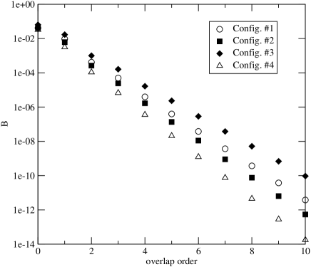
Figure 4.2: Breaking of the Ginsparg-Wilson relation for the overlap Dirac operator with FP kernel on different $10^{4}$ configurations at $\beta=3.2$. Only the smallest 10 eigenvalues are treated exactly.

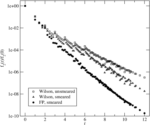
Figure 4.3: Locality of overlap Dirac operators with Wilson and FP kernels given by the exponential decrease of couplings with distance in Eq. (4.5). The Wilson operator is examined both on smeared and unsmeared gauge configurations with $\beta=3.0$. The plot is taken from [6].

4.2 Locality of Couplings

Every reasonable lattice Dirac operator has to be local, with exponentially decreasing couplings. If the Dirac operator is restricted to a finite number of lattice sites, like the Wilson or the parametrized FP Dirac operator, it is called ultralocal. The overlap construction takes an ultralocal operator as an input, but the result is no longer ultralocal. For the Wilson kernel, locality of the resulting overlap operator has been shown, but the exponential decay rate of the couplings is quite small. In Fig. 4.3 we compare the locality, measured by

$$f(r)=\underset{y}{\rm max}\{|D\cdot v|;||y-x||=r\},$$ (4.5)

where $v$ is vector with a point source at $x$, for the overlap Dirac operator with the Wilson and the FP kernel. Together with other tests for the locality of the Wilson overlap operator [42, 86], it follows that the locality is significantly improved when the FP kernel is used.

4.3 Locality of Instanton Zero Modes

The properties of approximately or exactly chiral Dirac operators can be tested on smooth instanton gauge configurations. Phenomenological models suggest that instantons might be responsible for dynamical chiral symmetry breaking [87]. Single instantons, which are gauge configurations with topological charge $Q=1$, produce a zero mode of the Dirac operator through the index theorem (2.9). A pair of an instanton and an anti-instanton produces two complex-conjugate near-zero eigenmodes. The chiral condensate, which is the order parameter for chiral symmetry breaking, is related to the density of eigenvalues of the Dirac operator near the origin through the Banks-Casher relation. In the infinite volume limit, the density of exact zero modes becomes negligible compared to the density of near-zero modes. Only with the contribution of near-zero modes, the eigenvalue density at zero therefore does not vanish at infinite volume. Initiated by [88], many groups have recently studied whether the local chirality properties of these near-zero modes are consistent with the instanton model of chiral symmetry breaking [89, 90, 91, 5].

In this section, we analyze eigenvalues and eigenvectors of the overlap-improved FP Dirac operator on gauge configurations describing a discretized exact instanton, as done in [92] for the chirally improved Dirac operator. For the above mentioned studies on local chirality, it is helpful to know how well a given Dirac operator reproduces the continuum zero mode of an instanton. We show that the Wilson overlap Dirac operator is in this respect not optimal, which might be due to its comparably bad locality properties. The gauge configurations are constructed from discretized $SU(2)$-instantons trivially embedded as $2\times 2$-submatrices in $SU(3)$ [92]. We work on lattices of size $12^{4}$ and apply antiperiodic boundary conditions in time for the fermions. Eigenvalues and eigenvectors are calculated with the implicitly restarted Arnoldi algorithm [93].

First, we compare the flow of the zero eigenvalue with instanton size for various Dirac operators in Fig. 4.4. For an exactly chiral operator (and also for the overlap-improved FP operator on the scale of this plot), the eigenvalue is exactly zero. Due to the residual chiral symmetry breaking, it can move away from zero for approximately chiral Dirac operators. The eigenvalue is however restricted to the real axis, as long as the Dirac operator respects $\gamma_{5}$-hermiticity. For varying instanton radius $\rho$, the position $x$ of the zero eigenvalue on the real axis can be monitored, providing a measure for the chiral properties of the Dirac operator.

For the Wilson operator, the eigenvalue quickly flows away from zero towards the center of the circle with decreasing instanton radius $\rho$. Calculating only the few smallest eigenmodes, we lost track of it already at $a\rho<2$. The parametrized FP Dirac operator shows a much better behavior, with the eigenvalue staying close to zero. For $a\rho<1.25$, it even moves back and takes a negative value at $a\rho=0.5$. This can be interpreted as an ’overimprovement’ caused by the fairly large coefficients for the fluctuation polynomials [6] in our parametrization: If at some locations the gauge fields fluctuate very strongly, as it is the case for such an artificial small instanton, the fluctuation polynomials shift the couplings in the Dirac operator away from reasonable values. The histogram of plaquette values in Fig. 4.5 illuminates the qualitative difference of the fluctuations in these instanton and in thermal Monte Carlo gauge configurations. While on a Monte Carlo configuration the plaquette distribution is smooth, most of the plaquettes of an instanton configuration are very close to $u=3$, but there is also a peak at $u\approx 1.6$ from the plaquettes at the center of the instanton. As a consequence, the Dirac operator is strongly affected there through the fluctuation polynomials which are proportional to terms like $3-u$, causing this unusual behavior of the real eigenvalue. We never observed such real eigenvalues shifted towards negative values in Monte Carlo gauge configurations used in actual lattice simulations, which were also used to parametrize the FP operator. Only in such an artificial environment as given by the discretized instantons the parametrized FP Dirac operator shows this effect.

We also investigate the effect of smearing for the FP operator. Obviously the RG inspired smearing, which we use together with the FP Dirac operator, does not change the flow of the real eigenvalue much. Only for the smallest instanton $a\rho=0.5$ the eigenvalue is pushed back slightly towards zero when the gauge configurations are smeared. Another approximately chiral operator that behaves very well on these instanton configurations is the chirally improved Dirac operator by Gattringer et al. [92], which is optimized for fulfilling the Ginsparg-Wilson relation.

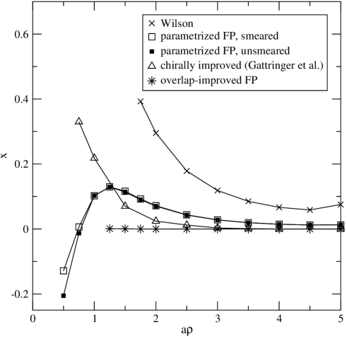
Figure 4.4: Position $x(a\rho)$ of the zero eigenvalue on the real axis in dependence of the instanton radius for different Dirac operators.

Figure 4.5: Histogram of plaquette values $u={\rm Re\ Tr\ }U_{\mu\nu}$ on a RG smeared Monte Carlo configuration at $\beta=3.0$ (smooth curve) and on a small, RG smeared instanton with $a\rho=0.5$ (peaks).

As a second check we investigate the locality properties of the corresponding zero eigenmode $\phi_{0}$, which is centered at the place where the instanton sits. With the gauge invariant density

$$p(x)\equiv\sum_{\alpha,a}\phi_{0}^{\alpha a}(x)^{*}\phi_{0}^{\alpha a}(x)\stackrel{{\scriptstyle\rm cont.}}{{=}}\frac{2\rho^{2}}{\pi^{2}(\rho^{2}+x^{2})^{3}},$$ (4.6)

where $\int d^{4}x\ p(x)=1$ for normalized eigenvectors, we can define as a measure for the localization of the zero mode $\phi_{0}$ the inverse participation ratio

$$I\equiv\int\!d^{4}x\ p(x)^{2}\stackrel{{\scriptstyle\rm cont.}}{{=}}\frac{1}{5\pi^{2}\rho^{4}},$$ (4.7)

which is plotted in Fig. 4.6 and compared to the continuum value. All Dirac operators agree for the largest instanton radii $\rho\geq 4$, where the lattice results deviate from the continuum due to finite-volume effects. The Wilson overlap operator however deviates strongly from the continuum values also for smaller instantons, seemingly having problems to reproduce the continuum zero mode. This can be interpreted as a consequence of the relatively bad localization properties of the overlap with Wilson kernel. Varying the optimizing parameter $s$ in the Wilson overlap does not lead to a significant change in these result [92]. The situation is different for the ultralocal Dirac operators like the parametrized FP and the Wilson operator. The parametrized FP operator reproduces the continuum value well even for very small instantons, while the Wilson operator performs somewhat worse, but still much better than the Wilson overlap.

The main result from this study is that the third order overlap-improved FP Dirac operator almost shows no change compared to the parametrized FP operator and captures the localization of the zero mode very well. The same observation has been made for an overlap operator with a chirally improved kernel, giving evidence that the Wilson kernel for the overlap construction, which misses the localization properties of the instanton zero mode, is not the best choice. Another observation we make when comparing the parametrized FP operator on both smeared and unsmeared gauge configurations is that the RG-inspired smearing of the gauge fields does not change the results for the inverse participation ratio. The smearing therefore does not seem to lead to a significant modification of the locality properties of the Dirac operator.

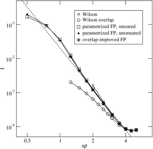
Figure 4.6: Inverse participation ratio $I(a\rho)$ of the zero eigenmode in dependence of the instanton radius for different Dirac operators. The values for the Wilson overlap are taken from [92]. The dashed line denotes the continuum value as given in Eq. (4.7).

Chapter 5 Hadron Spectroscopy in Lattice QCD

Among the most basic quantities that are calculable in lattice QCD are the masses and decay constants of the various bound states of quarks and gluons. Reproducing the experimentally observed spectrum of hadronic particles is one of the strongest tests that QCD is the correct theory to describe nature at the corresponding energy scale. In this chapter we present how masses of light hadrons, which are made from up, down and strange quarks, are extracted from quantities accessible on the lattice, and we discuss some refinements to improve the quality of these measurements.

First we derive in Section 5.1 the basic observation that the exponential decay of hadronic correlation functions is related to the hadron mass. The correlators can be calculated by inverting the lattice Dirac operator and contracting the resulting quark propagators together with the Dirac matrices corresponding to a particular hadronic state. Then we show in Section 5.2 how the overlap of the creation and annihilation operators with the ground state of the hadron can be increased by using extended wave functions at the source and sink locations. In the last section, we concentrate on the technical issues related to the fitting of lattice data to the predicted functional forms and show how the statistical error of the resulting hadron masses is estimated.

5.1 Fermionic Observables from Correlation Functions

The typical quantity to measure in lattice hadron spectroscopy is the two-point function

$$C(x)\equiv\langle 0|T\{{\mathcal{O}}_{f}(x){\mathcal{O}}^{\dagger}_{i}(0)\}|0\rangle,$$ (5.1)

describing the space-time propagation of a particle created at the origin by the operator ${\mathcal{O}}^{\dagger}_{i}$ and annihilated at space-time coordinate $x=(\vec{x},t)$ by the operator ${\mathcal{O}}_{f}$. To create a meson, a quark bilinear operator of the form

$${\mathcal{O}}^{\rm M}(x)\equiv\bar{\psi}^{a,f_{1}}_{\mu}(x)\Gamma_{\mu\nu}\psi^{a,f_{2}}_{\nu}(x),$$ (5.2)

is used. The Clifford algebra element $\Gamma$ determines the quantum numbers of the desired quark-antiquark state, and $f_{1}$, $f_{2}$ denote the flavors $u$,$d$,$s$ of the quark constituents. A baryon is created by the three-quark operator

$${\mathcal{O}}^{\rm B}(x)\equiv\epsilon_{abc}\chi_{\mu\nu\rho}\psi_{\mu}^{a,f_{1}}(x)\psi_{\nu}^{b,f_{2}}(x)\psi_{\rho}^{c,f_{3}}(x),$$ (5.3)

with some appropriate spin function $\chi_{\mu\nu\rho}$. In the simulations in Chapter 7, we will work with the baryon operators used by the MILC collaboration [97], which create an equal mixture of a forward propagating baryon and a backward propagating antibaryon on a periodic lattice. In Tables 5.1 and 5.2 we list the spin content of our meson and baryon operators.

Label	State	$I^{G}(J^{PC})$	Operator
S	scalar	$1^{-}(0^{++})$	$\bar{u}(x)d(x)$
P	pseudoscalar	$1^{-}(0^{-+})$	$\bar{u}(x)\gamma_{5}d(x)$
A		$1^{-}(0^{-+})$	$\bar{u}(x)\gamma_{4}\gamma_{5}d(x)$
V	vector	$1^{+}(1^{--})$	$\bar{u}(x)\gamma_{i}d(x)$

Table 5.1: Local interpolating field operators for mesons. In the vector meson, the sum over all polarizations $i=1,\dots,3$ is taken.

Label	State	Operator
N	octet, $|{\rm n},s_{3}=\frac{1}{2}\rangle$	$(d^{a}{\mathcal{C}}\gamma_{5}u^{b})u^{c}_{1}\epsilon_{abc}$
N0		$(d^{a}{\mathcal{C}}\gamma_{4}\gamma_{5}u^{b})u^{c}_{1}\epsilon_{abc}$
D	decuplet, $|\Delta^{+},s_{3}=\frac{3}{2}\rangle$	$2(d^{a}{\mathcal{C}}\gamma^{-}u^{b})u^{c}_{1}\epsilon_{abc}+(u^{a}{\mathcal{C}}\gamma^{-}u^{b})d^{c}_{1}\epsilon_{abc}$
D0		$2(d^{a}{\mathcal{C}}\gamma_{4}\gamma^{-}u^{b})u^{c}_{1}\epsilon_{abc}+(u^{a}{\mathcal{C}}\gamma_{4}\gamma^{-}u^{b})d^{c}_{1}\epsilon_{abc}$

Table 5.2: Local interpolating field operators for baryons. The charge conjugation matrix is ${\mathcal{C}}=\gamma_{2}\gamma_{4}$.

Let us demonstrate how to extract physical quantities from the correlation function (5.1) on a lattice of infinite volume. In order to single out particles with defined momenta, consider the spatial Fourier transform

$$C(\vec{p},t)=\sum_{\vec{x}}e^{i\vec{p}\vec{x}}\langle 0|T\{{\mathcal{O}}_{f}(\vec{x},t){\mathcal{O}}^{\dagger}_{i}(0,0)\}|0\rangle.$$ (5.4)

Inserting a complete set of eigenstates $|n,\vec{q}\rangle$ with spatial momentum $\vec{q}$, we get

$$C(\vec{p},t)=\sum_{\vec{x}}e^{i\vec{p}\vec{x}}\sum_{n}\int\frac{d^{3}\vec{q}}{(2\pi)^{3}2E_{n}(\vec{q})}\langle 0|{\mathcal{O}}_{f}(\vec{x},t)|n,\vec{q}\rangle\langle n,\vec{q}|{\mathcal{O}}^{\dagger}_{i}(0,0)|0\rangle,$$ (5.5)

where $E_{n}(\vec{q})$ is the energy of the intermediate state $|n,\vec{q}\rangle$. Applying the space-time translation ${\mathcal{O}}_{f}(x)=e^{i{\mathcal{P}x}}{\mathcal{O}}_{f}(0)e^{-i{\mathcal{P}x}}$ with four-momentum ${\mathcal{P}}=({\mathcal{H}},\vec{\mathcal{P}})$ to the annihilation operator, the correlation function (5.5) can be written as an exponentially weighted sum over all intermediate states,

$$C(\vec{p},t) =\sum_{n}\int\frac{d^{3}\vec{q}}{(2\pi)^{3}2E_{n}(\vec{q})}e^{-iE_{n}(\vec{q})t}\langle 0|{\mathcal{O}}_{f}|n,\vec{q}\rangle\langle n,\vec{q}|{\mathcal{O}}^{\dagger}_{i}|0\rangle\sum_{\vec{x}}e^{i(\vec{p}-\vec{q})\vec{x}}$$

$$=\sum_{n}\frac{\langle 0|{\mathcal{O}}_{f}|n,\vec{p}\rangle\langle n,\vec{p}|{\mathcal{O}}^{\dagger}_{i}|0\rangle}{2E_{n}(\vec{p})}\ e^{-iE_{n}(\vec{p})t},$$ (5.6)

where $\sum_{\vec{x}}e^{-i\vec{p}\vec{x}}=(2\pi)^{3}\delta(\vec{p})$ has been used to get rid of one momentum variable, and ${\mathcal{O}}_{i,f}\equiv{\mathcal{O}}_{i,f}(0,0)$. For large Euclidean time $\tau=it$, only the state with lowest energy contributes, therefore the asymptotic form of the correlation function becomes

$$C(\vec{p},\tau)\xrightarrow{\tau\rightarrow\infty}\frac{\langle 0|{\mathcal{O}}_{f}|1,\vec{p}\rangle\langle 1,\vec{p}|{\mathcal{O}}^{\dagger}_{i}|0\rangle}{2E_{1}(\vec{p})}\ e^{-E_{1}(\vec{p})\tau}.$$ (5.7)

Considering only intermediate states with zero momentum by setting $\vec{p}=0$, the mass of the lightest state can be extracted from the exponential decay of the Euclidean time correlation function

$$C(\tau)\xrightarrow{\tau\rightarrow\infty}\frac{A_{f}A_{i}^{*}}{2m_{1}}\ e^{-m_{1}\tau},$$ (5.8)

where the amplitudes $A_{i,f}=\langle 0|{\mathcal{O}}_{i,f}|1\rangle$ represent the overlap of the operators ${\mathcal{O}}_{i,f}$ with the lightest particle state having the quantum numbers of ${\mathcal{O}}_{i,f}$.

In Fig. 5.1, we plot typical examples of meson correlation functions on the lattice at varying quark masses, showing clearly the exponential decay with Euclidean time.

Figure 5.1: Pseudoscalar meson propagators $C(\tau)$ on a $16^{3}\times 32$ lattice for various quark masses. The data comes from our simulation at $\beta=3.0$ presented in Chapter 7. Due to the periodic boundary conditions, the correlators are symmetric around $\tau=16$.

5.1.1 Lattice Quark Propagators

In order to measure the correlation function (5.1) in lattice QCD, it is expressed in terms of the Euclidean quark propagator

$$G_{\mu\nu}^{ab}(x,y)\equiv\langle 0|T\{\psi_{\mu}^{a}(x)\bar{\psi}_{\nu}^{b}(y)\}|0\rangle,$$ (5.9)

using Wick contractions of the quark fields. Consider for example a flavor non-singlet meson operator (5.2), where $f_{1}\neq f_{2}$. The two-point function is then

$$\langle{\mathcal{O}}^{\rm M}(\vec{x},t){\mathcal{O}}^{\rm M{\dagger}}(0,0)\rangle \equiv\langle 0|T\{{\mathcal{O}}^{\rm M}(\vec{x},t){\mathcal{O}}^{\rm M{\dagger}}(0,0)\}|0\rangle$$

$$=\langle 0|T\{\bar{\psi}_{\sigma}^{a,f_{1}}(x)\Gamma_{\sigma\mu}\psi_{\mu}^{a,f_{2}}(x)\bar{\psi}_{\nu}^{b,f_{2}}(0)\Gamma_{\nu\rho}\psi_{\rho}^{b,f_{1}}(0)\}|0\rangle$$

$$=\langle G^{ab,f_{2}}_{\mu\nu}(x,0)\Gamma_{\nu\rho}G^{ba,f_{1}}_{\rho\sigma}(0,x)\Gamma_{\sigma\mu}\rangle$$

$$=\langle\operatorname{Tr}G^{f_{2}}(x,0)\Gamma G^{f_{1}}(0,x)\Gamma\rangle,$$ (5.10)

where the trace is taken over spin and color indices. Making use of the $\gamma^{5}$-hermiticity of the quark propagator $G(x,y)=\gamma^{5}G(y,x)^{\dagger}\gamma^{5}$, where the hermitean conjugation also acts in spin and color space, Eq. (5.1.1) becomes

$$\langle{\mathcal{O}}^{\rm M}(\vec{x},t){\mathcal{O}}^{\rm M{\dagger}}(0,0)\rangle=\langle\operatorname{Tr}G^{f_{2}}(x,0)\Gamma\gamma_{5}G^{f_{1}}(x,0)^{\dagger}\gamma_{5}\Gamma\rangle.$$ (5.11)

The importance of this last step comes from the fact that in lattice QCD calculations, the quark propagator $G(x,y)=D^{-1}(x,y)$ is determined by a matrix inversion of the lattice Dirac operator, which is by far the most expensive part of quenched simulations. A complete inversion amounts to solving the linear system of $12V$ equations

$$D_{\mu\nu}^{ab}(x,y)G_{\nu\rho}^{bc}(y,z)=\delta_{ac}\delta_{\mu\rho}\delta(x-z),$$ (5.12)

for $G$, which is in most cases not feasible. For the calculation of the right hand side of (5.11), it is however only necessary to know the quark propagator $G(x,0)$ from a fixed source point at the origin, where the particle is created, to all points on the lattice. Hence it is sufficient to evaluate 12 columns of the inverted matrix (one per spin and color) by solving

$$D_{\mu\nu}^{ab}(x,y)G_{\nu\rho}^{bc}(y,0)=\delta_{ac}\delta_{\mu\rho}\delta(x),$$ (5.13)

reducing the numerical size of the problem by a factor of $V$. This trick does not work in the case of flavor singlet mesons, where the disconnected contribution in the quark line graph requires the knowledge of the full quark propagator, which is the reason why their treatment on the lattice is much more demanding.

Finally, to get the zero momentum correlator (5.8), it is sufficient to sum Eq. (5.11) over all sink locations on a given timeslice,

$$C(\tau)=\Big{\langle}\sum_{\vec{x}}\operatorname{Tr}G^{f_{2}}(x,0)\Gamma\gamma_{5}G^{f_{1}}(x,0)^{\dagger}\gamma_{5}\Gamma\Big{\rangle},$$ (5.14)

which projects out the $\vec{p}=0$ contribution in (5.4).

5.2 Extended Source and Sink Operators

In order to get a good signal-to-noise ratio for the measured hadron correlators, the operators ${\mathcal{O}}_{i}$ and ${\mathcal{O}}_{f}$ in Eq. (5.1) should have a large overlap with the desired state. Local operators like (5.2) and (5.3) are not expected to fulfill this criterion well, as they do not take into account the spatial extension of the hadron. Especially for small quark masses or small lattice spacings, neglecting the hadron extension becomes a problem, as light hadrons typically have a size of $\mathcal{O}$(1 fm), and lattice spacings in current simulations are mostly between 0.05 fm and 0.2 fm. Maximum overlap for a meson would be reached for a non-local operator

$${\mathcal{O}}^{\rm M}_{\rm ext}(t)=\sum_{\vec{x},\vec{y}}\varphi(\vec{x},\vec{y})\bar{\psi}^{a,f_{1}}_{\mu}(\vec{x},t)\Gamma_{\mu\nu}\psi^{a,f_{2}}_{\nu}(\vec{y},t),$$ (5.15)

where $\varphi(\vec{x},\vec{y})$ is the wave function of the meson. For a delta function $\varphi(\vec{x},\vec{y})=\delta(\vec{x}-\vec{y})$, the local operator (5.2) is reproduced.

Spatially extended operators like (5.15) are often referred to as smeared operators. They are in this form not gauge invariant quantities, and therefore their average over gauge configurations would vanish due to Elitzur’s theorem [98]. To prevent that, one either has to include the parallel transporters in the operator or to work in a fixed gauge background. While gauge fixing is technically easy and imposes no restrictions on the wave function $\varphi(\vec{x},\vec{y})$, it introduces a possible source of errors due to the Gribov copy problem (see Appendix A). To avoid this problem, various kinds of gauge invariant operators like Jacobi-smeared [99] or Wuppertal sources [100, 101, 102], have been constructed. In the following however, we will concentrate on gauge non-invariant operators and measure them on gauge-fixed configurations, which is a common procedure adopted in many large-scale simulations [103, 104, 105, 106, 107, 108, 109].

The wave function $\varphi(\vec{x},\vec{y})$ of the simulated particle is a priori not known, so one has to make a more or less reasonable guess. A convenient, but not very physical choice is the totally factorized shell-model wave function [110, 111, 112]

$$\varphi(\vec{x},\vec{y})=\phi(\vec{x})\phi(\vec{y}),$$ (5.16)

where the quark and antiquark move independently inside a region given by the function $\phi(\vec{x})$, which might for example chosen to be a wall [113], a hard sphere or cube [110], a Gaussian [114, 115], or a radial exponential [106, 109]. General experience from lattice simulations has shown that using these kinds of extended operators, it is significantly easier to extract a reliable estimate for hadron masses from a fit to the correlation function (5.1), because due to the larger overlap with the ground state the contributions from higher states in (5.1) vanish at much smaller time separation $\tau$ than for local hadron operators [116, 106, 109, 117, 118, 103].

The advantage of the shell-model wave function (5.16) over more physical functions which depend on the relative coordinates between the quark and antiquark is that due to the factorization into separate quark and antiquark parts, the quark propagator can be calculated like for a local operator with only one inversion per spin and color. In the following, we suppose that $\phi(\vec{x})$ is a real, radial symmetric function,

$$\phi_{\vec{r}}(\vec{x})=\phi(||\vec{r}-\vec{x}||)$$ (5.17)

around a center $\vec{r}$ of the source or sink. Consider first a meson correlation function with a shell-model source operator (5.15)–(5.17)

$${\mathcal{O}}^{\rm M}_{\rm sm}(\vec{r},t)=\sum_{\vec{x},\vec{y}}\phi_{\vec{r}}(\vec{x})\bar{\psi}^{a,f_{1}}_{\mu}(\vec{x},t)\Gamma_{\mu\nu}\phi_{\vec{r}}(\vec{y})\psi^{a,f_{2}}_{\nu}(\vec{y},t),$$ (5.18)

at timeslice $t=0$ and centered at $\vec{r}=0$, and a local sink operator at time $t$:

$$\big{\langle}{\mathcal{O}}^{\rm M}(\vec{x},t){\mathcal{O}}^{\rm M{\dagger}}_{\rm sm} (0,0)\big{\rangle}=\Big{\langle}0\,\Big{|}\,\bar{\psi}^{f_{1}}(\vec{x},t)\Gamma\psi^{f_{2}}(\vec{x},t)$$

$$\hskip 51.21495pt\times\Bigl{(}\sum_{\vec{x}_{0},\vec{y}_{0}}\phi_{0}(\vec{x}_{0})\bar{\psi}^{f_{2}}(\vec{x}_{0},0)\Gamma\phi_{0}(\vec{y}_{0})\psi^{f_{1}}(\vec{y}_{0},0)\Bigr{)}^{\dagger}\,\Big{|}\,0\Big{\rangle}$$

$$=\Big{\langle}\operatorname{Tr}\sum_{\vec{x}_{0}}G^{f_{2}}(\vec{x},t;\vec{x}_{0},0)\phi_{0}(\vec{x}_{0})\Gamma\sum_{\vec{y}_{0}}G^{f_{1}}(\vec{y}_{0},0;\vec{x},t)\phi_{0}(\vec{y}_{0})\Gamma\Big{\rangle}$$

$$=\Big{\langle}\operatorname{Tr}G^{f_{2}}_{\rm sm}(\vec{x},t;0,0)\Gamma\gamma_{5}G^{f_{1}}_{\rm sm}(\vec{x},t;0,0)^{\dagger}\gamma_{5}\Gamma\Big{\rangle}.$$ (5.19)

The spatial distribution of the source is taken into account when inverting the Dirac operator on the vector $\phi_{0}(\vec{x})\delta(t)$ instead of $\delta(x)$, defining the smeared source quark propagator $G_{\rm sm}$ in Eq. (5.2) as the solution of

$$D(x,y)G_{\rm sm}(y,0)=\phi_{0}(\vec{x})\delta(t).$$ (5.20)

While introducing an extended source amounts to inverting the Dirac operator on a different source vector, using an extended sink leads to a weighting of the quark propagator at different lattice sites on a given timeslice, as can be seen from the smeared-source, smeared-sink meson correlator

$$\left\langle{\mathcal{O}}^{\rm M}_{\rm sm}(\vec{r},t){\mathcal{O}}^{\rm M{\dagger}}_{\rm sm}(0,0)\right\rangle=\Big{\langle}\operatorname{Tr}\sum_{\vec{x}_{t}}\phi_{\vec{r}}(\vec{x}_{t})G^{f_{2}}_{\rm sm}(\vec{x}_{t},t;0,0)\Gamma\gamma_{5}\\ \times\sum_{\vec{y}_{t}}\phi_{\vec{r}}(\vec{y}_{t})G^{f_{1}}_{\rm sm}(\vec{y}_{t},t;0,0)^{\dagger}\gamma_{5}\Gamma\Big{\rangle},$$ (5.21)

where the smearing of the source again is absorbed in the quark propagator.

As shown above, the hadron mass is extracted from the Fourier transform of the correlation function at zero momentum, which implies summing Eq. (5.21) over all sink locations $\vec{r}$. For a smeared sink, the numerical effort can get quite large, as there are then three sums over all lattice points on a given time slice. A technical trick to accelerate the calculation of smeared-sink meson correlators is to rewrite Eq. (5.21) in Fourier space, which allows to make use of efficient Fast Fourier Transform (FFT) algorithms to speed up the calculation. With the discrete Fourier representations of both the sink wave function

$$\phi_{\vec{r}}(\vec{x})=\frac{1}{N_{s}^{3/2}}\sum_{\vec{k}}e^{-i\frac{2\pi}{N}\vec{k}(\vec{r}-\vec{x})}\phi(\vec{k}),$$ (5.22)

where $k_{i}=0,\dots,N_{s}-1$ for $i=1,\dots,3$, and the quark propagator

$$G(\vec{x},t;0,0)=\frac{1}{N_{s}^{3/2}}\sum_{\vec{k}}e^{-i\frac{2\pi}{N}\vec{k}\vec{x}}G(\vec{k},t;0,0),$$ (5.23)

the convolutions in the meson correlator (5.21) can be expressed as

$$\sum_{\vec{x}}\phi_{\vec{r}}(\vec{x}_{t})G(\vec{x}_{t},t;0,0)=\sum_{\vec{k}}e^{-i\frac{2\pi}{N}\vec{k}\vec{r}}\phi(\vec{k})G(\vec{k},t;0,0),$$ (5.24)

leading to the zero-momentum smeared-source, smeared-sink meson correlator

$$\sum_{\vec{r}}\left\langle{\mathcal{O}}^{\rm M}_{\rm sm}(\vec{r},t){\mathcal{O}}^{\rm M{\dagger}}_{\rm sm}(0,0)\right\rangle=N_{s}^{3}\,\Big{\langle}\sum_{\vec{k}}\operatorname{Tr}\phi(\vec{k})G^{f_{2}}_{\rm sm}(\vec{k},t;0,0)\Gamma\gamma_{5}\\ \times\phi(\vec{k})G^{f_{1}}_{\rm sm}(\vec{k},t;0,0)^{\dagger}\gamma_{5}\Gamma\Big{\rangle}.$$ (5.25)

With this trick, the smeared-sink meson correlator at zero momentum is calculated in the same manner as the point-sink case (5.14) after replacing the 3-space fields by their Fourier transforms.

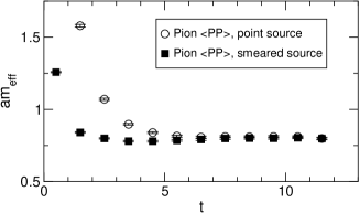
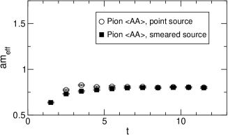
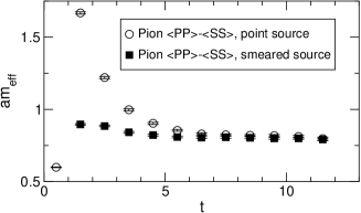
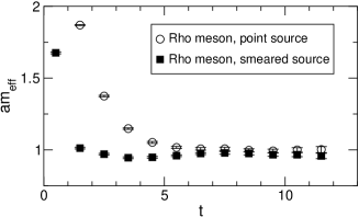
Figure 5.2: Effective mass plots for meson correlators with point and Gaussian smeared sources at bare quark mass $am=0.23$. The lattice size is $9^{3}\times 24$, the lattice spacing $a=0.16$ fm, and the data comes from 70 configurations evaluated with the FP Dirac operator. Although the lattice spacing is rather large, a clear enlargement of the plateau can be seen for all but the zero component axial vector $\langle AA\rangle$ correlator for the pion.

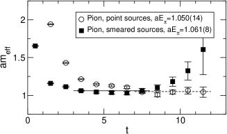
Figure 5.3: Effective energy plots at momentum $|ap|=2\pi/9$ for meson correlators with point and smeared sources. The simulation parameters are the same as in Fig. 5.2. The straight and dashed lines denote the time interval where the fit is done for the smeared and point sources. The statistical error for the fit results $aE_{\pi}$ and $aE_{\rho}$ is considerably smaller using smeared sources.

The effect of improving the overlap of the interpolating operators with the desired hadron state can be seen in the effective mass plots in Fig. 5.2. Compared are effective masses of pseudoscalar and vector mesons at large quark mass $am=0.23$ and lattice spacing $a=0.16$ fm for meson correlators made with point and Gaussian smeared sources, respectively. In both cases point sinks were chosen, and 70 gauge configurations of lattice size $9^{3}\times 24$ were used. The Gaussian smearing is defined by the shell-model wave function

$$\phi_{\vec{r}}(\vec{x})=e^{-\gamma(\vec{x}-\vec{r})^{2}},$$ (5.26)

and the source center $r_{i}=N_{i}/2$ with $i=1,\dots,3$ is located at the center of the time slice. The extension of the source used in the plots is given by $\gamma=0.15$. The plateau in the effective mass starts much earlier in most cases for smeared sources, providing a larger time interval over which the correlators can be fitted. The lattice spacing in the plots is rather large, and the effect will be enhanced at smaller $a$, where the point source correlators might not even reach a plateau within the given number of temporal lattice points. Fig. 5.3 shows plots for the effective energy of the pseudoscalar and vector meson at the lowest non-zero momentum $|ap|=2\pi/9$. There the signal is worse, and the length of the plateau for smeared correlators is only slightly increased, as the signal starts to deviate at large $t$. However, again the plateau region starts much earlier when using smeared sources, thus raising the confidence in that really the asymptotic behavior of the correlator is reached. Also, the statistical error of the energy resulting from the fit is significantly smaller for the smeared source correlators.

5.3 Fitting Hadron Propagators

As we have shown, hadron masses are extracted from the exponential fall-off of Euclidean time correlation functions at zero momentum (5.8), which are expressed in terms of the quark propagator and can thus be evaluated on the lattice. Consider the case of flavor non-singlet mesons Eq. (5.14), of which the correlation function $C(t)$ is measured on a lattice of temporal size $T$ for all $0\leq t<T$. Using periodic boundary conditions, the data points can be fitted against the asymptotic form

$$\begin{split}C_{\infty}(t)&=Z\big{(}e^{-mt}+e^{-m(T-t)}\big{)},\\ &=2Ze^{-mT/2}\cosh\big{(}m(T/2-t)\big{)},\end{split}$$ (5.27)

of the meson correlator in Euclidean time $t$ in order to determine the mass $m$ and the coefficient

$$Z=\frac{A_{f}A_{i}^{*}}{2m},$$ (5.28)

containing the information on the matrix elements of the chosen operators between the vacuum and the hadron state.

In order to find out at what time $t_{0}$ the asymptotic range of the hadron propagator is reached, it is helpful to plot the effective mass $m_{\rm eff}(t+1/2)$, which is determined from a zero parameter fit of the asymptotic function $C_{\infty}(t)$ to the measured propagators $C(t)$ and $C(t+1)$ at two consecutive time slices. When $t$ gets large enough that the higher lying states have disappeared, $m_{\rm eff}$ starts to show a plateau. In general, only the measured correlators in a time interval $t\in[t_{0},t_{1}]$ are then used to fit the parameters. The upper bound $t_{1}$ can be set to the point where the signal disappears in the statistical noise, which happens for all particles but pseudoscalar mesons after a certain temporal range.

In Figs. 5.5–5.8, we show examples of effective masses, fitted masses and the quality of the fit given by the value of $\chi^{2}/df$ for several particles at intermediate quark mass. In all cases, $t_{1}$ was set to $T/2$. For all hadrons, $\chi^{2}/df$ quickly decreases and stays then at a value of order 1, and the optimal fit interval starts in the range $3\leq t_{0}\leq 6$.

5.3.1 Correlated Fits

Suppose we have measured the hadron propagators $C^{(i)}(t)$ for $t=0,\dots,T$ on $N$ independent, importance sampled gauge configurations $U^{(i)}$ with $i=1,\dots,N$. Trying to fit the gauge average $\overline{C}(t)=1/N\sum_{i}C^{(i)}(t)$, we are faced with the problem that while the data is uncorrelated in Monte Carlo time $i$, it is strongly correlated in the temporal direction. The goal is to find the optimal parameters $m$ and $Z$ in the asymptotic form (5.27), taking into account the time correlations. This is done by minimizing the $\chi^{2}$-function

$$\chi^{2}=\sum_{t,t^{\prime}}\left\{\overline{C}(t)-C_{\infty}(t;m,Z)\right\}\,({\rm Cov})^{-1}(t,t^{\prime})\,\left\{\overline{C}(t^{\prime})-C_{\infty}(t^{\prime};m,Z)\right\},$$ (5.29)

where the time correlations are encoded in the symmetric, positive definite covariance matrix

$$({\rm Cov})(t,t^{\prime})=\frac{1}{N(N-1)}\sum_{i=1}^{N}\big{(}C^{(i)}(t)-\overline{C}(t)\big{)}\big{(}C^{(i)}(t^{\prime})-\overline{C}(t^{\prime})\big{)}.$$ (5.30)

As an illustration of the typical size of time correlations we plot a row of the normalized correlation matrix

$$\Sigma(t,t^{\prime})=\frac{({\rm Cov})(t,t^{\prime})}{\sqrt{({\rm Cov})(t,t)({\rm Cov})(t^{\prime},t^{\prime})}},$$ (5.31)

for different smeared-source hadron propagators in Fig. 5.4. The data is strongly correlated for all hadrons under consideration. For the pseudoscalar meson, the time correlations do not die out at large $t$, as the signal-to-noise ratio remains constant, whereas for the other hadrons what mostly remains is uncorrelated statistical noise. The time correlations of pseudoscalar propagators are even stronger for point sources [120], therefore it is in any case mandatory to perform correlated fits by including the covariance matrix.

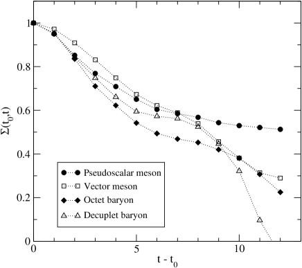
Figure 5.4: Temporal correlations of hadron correlators for a typical time range used in mass fits. The correlators are from $N=100$ independent gauge configurations of size $16^{3}\times 32$ at $\beta=3.0$ with smeared sources and point sinks, the quark mass is $am=0.18$ and the time interval starts at $t_{0}=4$.

5.3.2 Resampling Methods for Error Estimates

The results of the above described procedure are the parameters of the fit function, that is the hadron mass $m$ and the amplitude $Z$. Since these fit parameters are statistical estimates from a Monte Carlo integration, it is necessary to provide an estimate of their statistical errors in order to judge their reliability. The measured observables are the hadron correlators, and what is needed is a tool to estimate the errors of quantities which depend in a complicated way on these observables. For the sample mean of the correlators, the standard deviation can be calculated in the usual way,

$$\sigma_{\overline{C}}=\left(\frac{1}{N(N-1)}\sum_{i=1}^{N}(C^{(i)}-\overline{C})^{2}\right)^{1/2},$$ (5.32)

but for less trivial functions of the observables, there is no such function to estimate the error. With the advent of powerful computers, robust statistical methods have been developed which allow to estimate errors of arbitrarily complicated functions of observables with unknown probability distributions in a straightforward way. These widely used methods are known under the names jackknife and bootstrap, and they are both based on resampling of the measured data. We briefly present the jackknife and the bootstrap resampling techniques in the following.

Suppose we have a set of $N$ independent and identically distributed measurements

$$X_{1},\dots,X_{N}\stackrel{{\scriptstyle\rm iid}}{{\sim}}F,$$ (5.33)

following an unknown distribution function $F$. From these data points, an arbitrarily complicated secondary quantity $\hat{\theta}(X_{1},\dots,X_{N})$ is calculated. What we aim at is an expression for the standard deviation $\sigma_{\hat{\theta}}(F)$ of the estimator $\hat{\theta}$. Jackknife resampling requires to calculate the estimator

$$\hat{\theta}_{(i)}=\hat{\theta}(X_{1},\dots,X_{i-1},X_{i+1},\dots,X_{N}),$$ (5.34)

on the sample where the data point $X_{i}$ has been dropped, for all $i=1,\dots,N$. The jackknife estimate for the error of $\hat{\theta}$ is then defined by

$$\sigma_{\hat{\theta}}^{\rm jack}=\left(\frac{N-1}{N}\sum_{i=1}^{N}(\hat{\theta}_{(i)}-\hat{\theta}_{(\cdot)})^{2}\right)^{1/2},$$ (5.35)

where $\hat{\theta}_{(\cdot)}=\sum_{i=1}^{N}\hat{\theta}_{(i)}/N$ is the average of the estimator over all jackknife samples.

The jackknife utilizes only $N$ of the $2^{N}-1$ non-empty subsets of the data set. The error estimate might thus be improved when more of the subsets are used. This lead to the development of the bootstrap [121]: A bootstrap sample

$$X^{*}_{1},\dots,X^{*}_{N}\stackrel{{\scriptstyle\rm iid}}{{\sim}}\hat{F},$$ (5.36)

is a random sample drawn with replacement from the observed values $X_{1},\dots,X_{N}$ and follows the empirical probability distribution $\hat{F}$ of the data. The bootstrap error estimate for $\hat{\theta}$ is defined from the estimator $\hat{\theta}^{*}=\hat{\theta}(X^{*}_{1},\dots,X^{*}_{N})$ calculated on $B$ bootstrap samples by

$$\sigma_{\hat{\theta}}^{\rm boot}=\left(\frac{1}{B-1}\sum_{b=1}^{B}(\hat{\theta}^{*}_{(b)}-\hat{\theta}^{*}_{(\cdot)})^{2}\right)^{1/2},$$ (5.37)

where $\hat{\theta}^{*}_{(\cdot)}=\sum_{b=1}^{B}\hat{\theta}^{*}_{(b)}/B$ denotes the average over the bootstrap samples. In the limit $B\rightarrow\infty$, the bootstrap error is exactly the standard deviation of the estimator as a function of the empirical probability distribution $\hat{F}$,

$$\sigma_{\hat{\theta}}^{\rm boot}\xrightarrow{B\rightarrow\infty}\sigma_{\hat{\theta}}(\hat{F})\approx\sigma_{\hat{\theta}}(F).$$ (5.38)

In practice, the number of bootstrap samples $B$ is finite, and one has to make sure that it is large enough by varying $B$ and checking whether the error changes significantly. But since $\hat{F}$ is only an estimate for the unknown probability distribution $F$, taking too many bootstrap samples does not help improving the error estimate for $\sigma_{\hat{\theta}}(F)$. For most cases, it is considered safe to work with values in the range $100<B<500$. In our spectroscopy simulations, the computational cost for the bootstrap is negligible, and therefore we always calculate $B=1000$ bootstrap samples.

The jackknife and bootstrap procedures also provide an estimate for the bias $\hat{b}_{\hat{\theta}}$ of the estimator $\hat{\theta}$. The jackknife estimate of bias is given by

$$\hat{b}^{\rm jack}_{\hat{\theta}}=(N-1)(\hat{\theta}_{(\cdot)}-\hat{\theta}),$$ (5.39)

while for the bootstrap it is just the difference of the value of the estimator on the original sample and its mean value on the bootstrap samples,

$$\hat{b}^{\rm boot}_{\hat{\theta}}=\hat{\theta}^{*}_{(\cdot)}-\hat{\theta}.$$ (5.40)

The bias-corrected estimator $\tilde{\theta}=\hat{\theta}-\hat{b}$ might then be used instead of $\hat{\theta}$ for a better estimate of the true value $\theta$.

Figure 5.5: Effective mass $m_{\rm eff}(t)$, fitted mass $m_{\rm fit}(t_{0})$ from a correlated fit in the range $[t_{0},16]$ and the value of $\chi^{2}/df$ for the fit (from bottom to top) for the pseudoscalar meson at $am=0.09$, $\beta=3.0$ and lattice size $16^{3}\times 32$. Error bars are from a bootstrap resampling of the propagators.

Figure 5.6: The same as Fig. 5.5 for the vector meson.

Figure 5.7: The same as Fig. 5.5 for the octet baryon.

Figure 5.8: The same as Fig. 5.5 for the decuplet baryon.

Chapter 6 Topological Finite-Volume Artifacts in Pion Propagators

In the chiral limit of quenched QCD, pion propagators suffer from unphysical quenching effects which make a thorough examination of light pions difficult. These quenching artifacts are caused by zero eigenmodes of the Dirac operator and lead to unphysical divergences of the pion propagators at $m\rightarrow 0$. In unquenched QCD, gauge configurations with zero modes are suppressed by the fermion determinant in the effective action, therefore these divergences are absent. Because the determinant is set to unity in the quenched theory, the suppression falls away, and at small quark mass the propagators are dominated by the zero mode effects. This can be clearly seen in Fig. 6.1, where the chiral limit of $m_{\rm PS}^{2}(m_{q})$ is shown in dependence of the topology of the gauge configurations. While the pseudoscalar meson mass goes to zero in the chiral limit on configurations with trivial topology, it deviates as soon as also configurations with non-zero topological charge are considered in the Monte Carlo average.

For the study of light pseudoscalar mesons with masses around the physical mass of the pion, it is therefore unavoidable to get rid of these artificial effects. In particular for the investigation of quenched chiral logarithms in the pseudoscalar mass, which we undertake in Chapter 7, the effects from zero modes have to be properly disentangled from the chiral logarithm, which produces a measurable signal only at small quark masses. Due to the explicit breaking of chiral symmetry, traditional formulations of lattice fermions like Wilson or Symanzik-improved clover fermions do not allow to identify topological zero modes unambiguously. Only with the development of chiral symmetric lattice Dirac operators, it has become possible to identify the zero modes responsible for these unwanted effects.

In a study with the Wilson overlap operator [85], the authors have reported a change in the behavior of the pseudoscalar correlator at large time, suggesting that the zero modes only contaminate the small $t$ range. As a possible solution, they proposed to fit the mass from the large $t$ tail of the correlator. Fig. 6.2 shows the reported kink in the correlator as seen in our data, but even a fit to the flatter region does not give a pion mass which goes to zero in the chiral limit. Furthermore, we could not clearly identify such a kink in all our simulations.

In this chapter we derive and examine two other solutions of the problem. One solution is based on explicit identification and subtraction of the zero modes in the quark propagator. The other solution, originally proposed in [45], makes use of the fact that zero mode effects enter pseudoscalar and scalar meson propagators equivalently. The zero mode effects can then be subtracted in the meson propagators. We study these two solutions on a very small lattice of spatial physical extension $L_{s}\approx 1$ fm, where the zero mode effects are large.

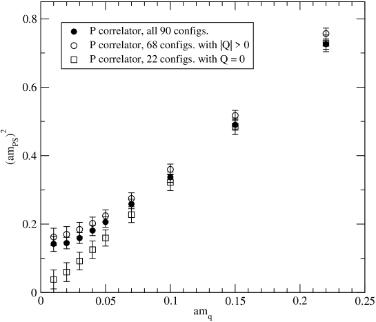
Figure 6.1: Chiral limit of the squared pion mass from pseudoscalar (P) correlators in dependence of gauge field topology. The overlap-improved FP Dirac operator is used on a set of 90 gauge configurations of size $6^{3}\times 16$ at $\beta=3.0$. At small quark mass, the pion evaluated on the full set is dominated by the configurations with non-trivial topology $|Q|>0$. If only the $Q=0$ configurations are considered, no quenched finite-volume artifacts are seen, and the pion mass goes to zero in the chiral limit.

Figure 6.2: The kink in the pseudoscalar correlator as reported in [85] from our data on the $12^{3}\times 24$ lattice at $a\approx 0.16$ fm and quark mass $am_{q}=0.01$. A closer examination shows that even if the fit interval $t\in[6,12]$ is chosen, which includes only the flatter part, the fitted mass $am_{\rm PS}=0.186(11)$ is still considerably larger than for the P-S correlator, where $am_{\rm PS}=0.136(22)$.

6.1 Zero Mode Subtraction of the Quark Propagator

The most straightforward way to get rid of zero mode contributions is to subtract them directly from the quark propagator. An exact subtraction however is only possible for an exactly chiral Dirac operator. We derive in the following the subtraction of the zero modes for the propagator of the overlap-improved FP Dirac operator described in Chapter 4, which is not trivial due to the Fixed-Point $R$ appearing in the Ginsparg-Wilson relation. From the subtracted quark propagators, meson and baryon correlators can be constructed in the standard way, and measurements of hadronic quantities derived from these correlators should then be free of quenched topological finite-volume artifacts.

6.1.1 Spectral Decomposition of the Massless Normal Dirac Operator

The overlap-improved FP Dirac operator is a solution of the Ginsparg-Wilson relation $\left\{D,\gamma_{5}\right\}=D\gamma_{5}2RD$, where a non-trivial $R$ appears on the right-hand side. Defining the operator

$$\tilde{D}\equiv\sqrt{2R}D\sqrt{2R},$$ (6.1)

the Ginsparg-Wilson relation reduces to the simpler case $\{\tilde{D},\gamma_{5}\}=\tilde{D}\gamma_{5}\tilde{D}$. With the $\gamma_{5}$-hermiticity of Dirac operators $D^{\dagger}=\gamma_{5}D\gamma_{5}$, it follows that $\tilde{D}$ is a normal operator,

$$\tilde{D}^{\dagger}\tilde{D}=\tilde{D}\tilde{D}^{\dagger}.$$ (6.2)

Normal operators can be written as diagonal matrices in an orthonormal basis of eigenvectors. Thus we can write down the spectral decomposition of a matrix element of the massless normal Dirac operator

$$\tilde{D}_{ij}=\sum_{\lambda}\lambda\tilde{\phi}_{\lambda}(i)\tilde{\phi}_{\lambda}^{\dagger}(j),$$ (6.3)

where $\lambda$ and $\tilde{\phi}_{\lambda}$ are the eigenvalues and the corresponding eigenvectors of $\tilde{D}$, and the indices $i$ and $j$ contain spin, color and space-time degrees of freedom. Since the inversion of a diagonal matrix is trivial, the spectral decomposition of the quark propagator $\tilde{G}_{ij}\equiv(\tilde{D}^{-1})_{ij}$ is given by

$$\tilde{G}_{kl}=\sum_{\lambda}\frac{1}{\lambda}\tilde{\phi}_{\lambda}(k)\tilde{\phi}^{\dagger}_{\lambda}(l).$$ (6.4)

The orthonormality condition on the eigenvectors reads

$$\sum_{l}\tilde{\phi}^{\dagger}_{\lambda}(l)\tilde{\phi}_{\lambda^{\prime}}(l)=\delta_{\lambda\lambda^{\prime}}.$$ (6.5)

We define the subtracted quark propagator by summing only over the non-zero eigenmodes of $\tilde{D}$,

$$\tilde{G}_{kl}^{(\rm sub)}\equiv\sum_{\lambda\neq 0}\frac{1}{\lambda}\tilde{\phi}_{\lambda}(k)\tilde{\phi}^{\dagger}_{\lambda}(l).$$ (6.6)

In presence of a finite mass, we will invert a matrix of the form $a\tilde{D}+b$ with $a,b\in{\bf R}$, and Eq. (6.6) can be written as

$$\tilde{G}_{kl}^{(\rm sub)}(a,b)=\tilde{G}_{kl}(a,b)-\sum_{\lambda=0}\frac{1}{b}\tilde{\phi}_{\lambda}(k)\tilde{\phi}^{\dagger}_{\lambda}(l).$$ (6.7)

6.1.2 Basis Transformation

For practical applications, it is not convenient to work with $\tilde{D}$ as defined in Eq. (6.1) due to the appearance of the square root of $2R$, whose calculation is a non-trivial numerical problem. A simple basis transformation

$$\hat{\phi}\equiv S\tilde{\phi},$$ (6.8)

with $S=(2R)^{-1/2}$ helps to get rid of this square root. The eigenvalues $\lambda$ remain unchanged under this transformation. The application of the basis transformed Dirac operator

$$\hat{D}\equiv S\tilde{D}S^{-1}=D2R,$$ (6.9)

on a vector is then reduced to multiplications with both D and R. From the definition (6.6),(6.7) we can read off the subtracted propagator in the new basis,

$$\hat{G}_{ij}^{(\rm sub)}(a,b)\equiv S\tilde{G}_{ij}^{(\rm sub)}(a,b)S^{-1}=\hat{G}_{ij}(a,b)-\sum_{\lambda=0}\frac{1}{b}\hat{\phi}_{\lambda}(i)\hat{\phi}^{\dagger}_{\lambda}(k)2R_{kj},$$ (6.10)

where $\hat{\phi}$ are eigenvectors of $\hat{D}$ and $\hat{G}_{kl}\equiv(\hat{D}^{-1})_{kl}$. We have to remark that due to the basis transformation, the Dirac operator $\hat{D}$ is no longer normal, and its eigenvectors are not orthogonal, but instead fulfill the generalized orthonormality condition

$$\sum_{k,l}\hat{\phi}^{\dagger}_{\lambda}(k)2R_{kl}\hat{\phi}_{\lambda^{\prime}}(l)=\delta_{\lambda\lambda^{\prime}}.$$ (6.11)

6.1.3 A Cookbook Recipe

The above discussion is valid for general massless Ginsparg-Wilson Dirac operators. We consider in the following the overlap-improved FP Dirac operator (4.1). After basis transformation (6.9), the mass dependence of $\hat{D}(m)$ is the usual one,

$$\hat{D}(m)\equiv\left(1-\frac{m}{2}\right)\hat{D}+m,$$ (6.12)

where the $2R$ in the denominator has disappeared.

With these ingredients, we are ready to give a cookbook recipe for the calculation of zero-mode subtracted quark propagators with the massive overlap-improved FP Dirac operator. These are the solutions of the equation

$$D_{kl}^{(\rm sub)}(m)g^{(\rm sub)}(k;m)=b(l),$$ (6.13)

where the subtracted Dirac operator is defined through Eqs. (6.9) and (6.10). The steps to find the solution $g^{(\rm sub)}(k;m)$ are the following:

1. Calculate the few smallest eigenmodes of $\hat{D}$,

   $$\hat{D}\hat{\phi}=D2R\hat{\phi}=\lambda\hat{\phi},$$ (6.14)

   identify the zero modes, where $\lambda=0$, and normalize them according to (6.11).

2. Invert $\hat{D}(m)$ on a source $b(y)$ by solving the equation

   $$\hat{D}_{xy}(m)\hat{g}(x;m)=b(y),$$ (6.15)

   for the vector $\hat{g}(x;m)$.

3. Subtract the zero modes from the solution $\hat{g}(x;m)$ as derived in Eq. (6.10):

   $$\hat{g}^{(\rm sub)}(x;m)=\hat{g}(x;m)-\sum_{\lambda=0}\frac{1}{m}\hat{\phi}_{\lambda}(x)\hat{\phi}^{\dagger}_{\lambda}(z)2R_{zy}b(y).$$ (6.16)

4. To get the inverse of $D$, multiply the result by $2R$:

   $$g^{(\rm sub)}(x;m)=2R\hat{g}^{(\rm sub)}(x;m).$$ (6.17)

We have to remark that in principle it would be more elegant to perform the basis transformation (6.8) in the inverse direction with $S=2R$, because then in the above steps 6.16 and 6.17 the factor of $2R$ disappears. The reason we do not follow this apparently simpler path is that in the orthonormality condition (and in hermitean forms in general, which are used in certain parts of our code), a multiplication with the inverse of $2R$ would show up, which is of course numerically much more demanding.

6.2 Zero Mode Contributions in Meson Propagators

Consider first the case of the normal Dirac operator $\tilde{D}$, where a spectral decomposition into a complete set of eigenstates is possible. Inserting the spectrally decomposed quark propagator (6.4) into the meson propagator (5.11), we get

$$\langle{\mathcal{O}}^{\rm M}(x){\mathcal{O}}^{\rm M{\dagger}}(0)\rangle=\sum_{\lambda,\lambda^{\prime}}\frac{\operatorname{Tr}\big{[}\tilde{\phi}_{\lambda}^{\dagger}(x)\Gamma\gamma_{5}\tilde{\phi}_{\lambda^{\prime}}(x)\big{]}\operatorname{Tr}\big{[}\tilde{\phi}_{\lambda^{\prime}}^{\dagger}(0)\Gamma^{*}\gamma_{5}\tilde{\phi}_{\lambda}(0)\big{]}}{(\lambda+m)(\lambda^{\prime}+m)},$$ (6.18)

where the color and spin indices have been suppressed and only the spatial index is given explicitly. Splitting the sum into three contributions and summing over $\vec{x}$ to project out zero momentum states leads to

$$\sum_{\vec{x}}\langle{\mathcal{O}}^{\rm M}(x){\mathcal{O}}^{\rm M{\dagger}}(0)\rangle=\sum_{\vec{x}}\left[\sum_{\lambda=\lambda^{\prime}=0}\frac{\operatorname{Tr}\big{[}\tilde{\phi}_{\lambda}^{\dagger}(x)\Gamma\gamma_{5}\tilde{\phi}_{\lambda^{\prime}}(x)\big{]}\operatorname{Tr}\big{[}\tilde{\phi}_{\lambda^{\prime}}^{\dagger}(0)\Gamma^{*}\gamma_{5}\tilde{\phi}_{\lambda}(0)\big{]}}{m^{2}}\right.\\ +\left.\sum_{\lambda=0,\,\lambda^{\prime}\neq 0}\frac{\operatorname{Tr}\big{[}\tilde{\phi}_{\lambda}^{\dagger}(x)\Gamma\gamma_{5}\tilde{\phi}_{\lambda^{\prime}}(x)\big{]}\operatorname{Tr}\big{[}\tilde{\phi}_{\lambda^{\prime}}^{\dagger}(0)\Gamma^{*}\gamma_{5}\tilde{\phi}_{\lambda}(0)\big{]}}{m(\lambda^{\prime}+m)}\right]+\sum_{n}\frac{|\langle 0|{\mathcal{O}}^{\rm M}|n\rangle|^{2}}{2E_{n}}\ e^{-E_{n}\tau}.$$ (6.19)

The first two summands, which are the pure and mixed zero mode contributions, are divergent in the chiral limit $m\rightarrow 0$. The zero mode contributions are finite volume artifacts expected to diverge with $1/\sqrt{V}$ [45], and the meson correlator diverges at finite volume with ${\mathcal{O}}(1/m^{2})$ and ${\mathcal{O}}(1/m)$ terms in the chiral limit. If the zero modes in the quark propagator have been subtracted as in Eq. (6.10), these divergences are absent, and also at small quark masses a good signal for the exponential decay of the meson mass can be obtained.

Let us discuss what happens for different meson operators. For the pseudoscalar, we have $\Gamma=\Gamma^{*}=\gamma_{5}$ with our definition of the Clifford matrices, while for the scalar meson $\Gamma=\Gamma^{*}=1$. The zero modes are chiral eigenstates with $\gamma_{5}\tilde{\phi}_{\lambda=0}=\pm\tilde{\phi}_{\lambda=0}$, hence it follows that the pseudoscalar and the scalar correlator have the same contributions from zero modes. By taking the difference between the two correlators, the zero mode contributions are therefore exactly cancelled. For the axial vector current correlator $\Gamma=\gamma_{4}\gamma_{5}$, the first summand in Eq. (6.19) is zero, since $\gamma_{4}$ couples different chiral sectors and all zero modes on a given gauge configuration have equal chirality. So for this correlator, the zero modes contribute only in the mixed term, and therefore it diverges only with $1/m$ in the chiral limit.

If we consider the non-normal Dirac operator $D$, we have $G=\sqrt{2R}\tilde{G}\sqrt{2R}$, and in the numerators of Eqs. (6.18) and (6.19) additional factors of $\sqrt{2R}$ show up. After subtracting the zero modes of $\tilde{D}$ according to (6.14)–(6.17), again the divergence in the chiral limit is no longer present.

6.3 Numerical Results at Small Volume

In order to examine the finite-volume zero mode effects in pion propagators, we perform an exploratory study with the overlap-improved FP Dirac operator on a very small lattice of size $6^{3}\times 16$ at gauge coupling $\beta=3.0$, with a set of 90 independent gauge configurations. This lattice volume amounts to a spatial extension of 1 fm, therefore the signal in the pseudoscalar channel is strongly affected by the zero modes. The Dirac operator is constructed with a third order Legendre expansion for the overlap and with exact treatment of the smallest 10 eigenmodes. Two different strategies are examined to remove the zero mode effects from the pion propagator:

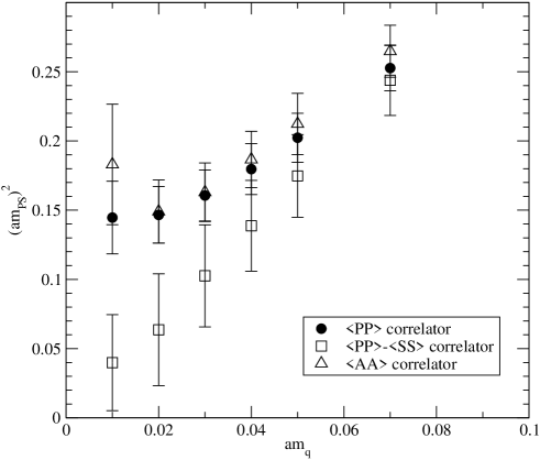
Figure 6.4: Topological quenching artifacts in squared pseudoscalar meson mass versus bare quark mass at $\beta=3.0$ and volume $6^{3}\times 16$. The effective masses at the smallest quark mass are shown in Fig. 6.3.

The first strategy is to remove the zero modes from the pseudoscalar (P) correlator by building the difference of the pseudoscalar and the scalar (P-S) correlator as described in Section 6.2. We further calculate the zero component axial vector (A) correlator, which also has the quantum numbers of the pion, and for which the zero mode contributions are partially cancelled. We show in Fig. 6.3 the effective masses at the smallest quark mass $am=0.01$ and in Fig. 6.4 the squared pion mass as a function of the quark mass. Obviously the different correlators give very different results at small quark mass. While the chiral limit of the pseudoscalar correlator clearly deviates from zero, it is consistent with zero for the P-S correlator. For the axial correlator, the zero mode effects are of the same order as for the pseudoscalar. For comparison, we show in Figs. 6.5 and 6.6 the same plots for a larger volume of $12^{3}\times 24$, with unchanged gauge coupling $\beta=3.0$, the same Dirac operator and 100 independent gauge configurations. There the zero mode effects are much smaller due to the larger physical volume. However, the pion mass from the pseudoscalar correlator still clearly deviates from zero in the chiral limit, while for the P-S correlator it nicely goes to zero. From these results we find that removing the zero mode effects in the pion at small quark mass by using the P-S correlator works fine.

The second strategy is to explicitly calculate the zero modes and remove them from the quark propagator as shown in Section 6.1. This is only possible if the Dirac operator allows to identify zero modes unambiguously. To check whether this requirement is fulfilled for the overlap-improved FP Dirac operator, we show in Table 6.1 for a gauge configuration with $Q=1$ the position of the zero eigenvalue on the real axis and the first non-zero eigenvalue as a function of the overlap order. We also list the chirality of the corresponding eigenvector $\phi^{(i)}$, defined by

$$\chi^{(i)}=\phi^{(i)}\gamma_{5}2R\phi^{(i)},$$ (6.20)

which is $\pm 1$ for zero modes. Obviously, it is easily possible to separate the zero mode and the first non-zero mode, even if the eigenvalue $\lambda_{0}$ is not very close to zero, because the chirality of the zero mode approaches $|\chi_{0}|\rightarrow 1$ very quickly with increasing order of the overlap expansion.

order	Re $\lambda_{0}$	$1-|\chi_{0}|$	Re $\lambda_{1}$	Im $\lambda_{1}$
0	-5.4e-03	2.4e-02	-3.782e-03	5.5974e-02
1	-3.1e-03	7.0e-04	-2.487e-03	5.5115e-02
2	5.1e-04	1.9e-05	2.148e-03	5.4854e-02
3	-2.1e-04	7.2e-07	1.300e-03	5.4901e-02
4	-2.5e-06	4.5e-08	1.508e-03	5.4890e-02
5	1.3e-06	3.7e-09	1.511e-03	5.4889e-02
6	-4.6e-07	8.1e-11	1.507e-03	5.4890e-02
7	3.6e-08	6.9e-12	1.508e-03	5.4890e-02

Table 6.1: Flow of the zero mode of a $Q=1$ gauge configuration, its chirality and the first near-zero mode with increasing overlap order. $({\rm Im}\ \lambda_{0})$ and $\chi_{1}$ are zero to machine precision.

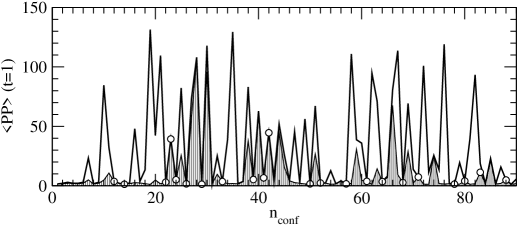
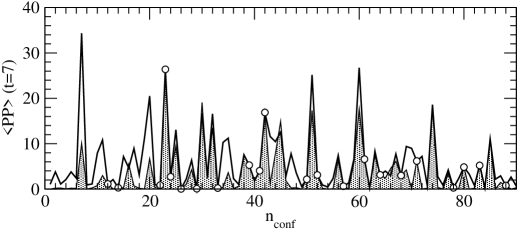
Figure 6.8: Monte Carlo time evolution of full (thick empty line) and zero mode subtracted (filled) pseudoscalar correlator at quark mass $am=0.01$. Shown are the correlators at times $t=1$ (top) and $t=7$ (bottom). Empty dots mark topologically trivial gauge configurations, where the correlators are equal.

We therefore calculate on every gauge configuration the eigenvectors $\phi^{(i)}$, $i=1,\dots,10$ of $\hat{D}$ corresponding to the 10 smallest eigenvalues and computed their chirality, and the eigenvectors with chirality $|\chi^{(i)}|\geq 0.9$ are considered to be zero modes. The distribution of the topological charge for the set of 90 gauge configurations is peaked at $Q=1$, as can be seen in Table 6.2. All zero modes are subtracted from the quark propagator according to (6.10), and with the subtracted quark propagators, pion propagators are constructed in the usual way. In the pseudoscalar correlator, the zero mode effects should then disappear, while the P-S correlator should remain unchanged. First we examine the correlators at the smallest quark mass $am=0.01$ in Fig. 6.7. The subtraction of the zero modes leads both to a strong decrease in the amplitude and the mass, as can be seen from the fitted lines. This effect is illustrated by the Monte Carlo time evolution of the pseudoscalar correlators in Fig. 6.8. At small time $t=1$, the correlator fluctuates wildly with Monte Carlo time. The zero mode subtraction removes most of the peaks at topologically non-trivial gauge configurations. The average over Monte Carlo time is therefore much smaller for the subtracted correlator. At large time $t=7$, the picture changes and more peaks remain after zero mode subtraction. Some of the most prominent peaks (no. 23 and 42) even are at $Q=0$ gauge configurations and therefore do not come from zero modes. The average correlator decreases only moderately after subtraction. Combining the observations at the two times, it follows that the pion mass gets smaller at $am=0.01$ when determined from the subtracted propagators.

The situation is different at very large quark mass $am=0.32$. The subtracted and unsubtracted pseudoscalar correlators in Fig. 6.9 are almost equivalent at small $t$, but clearly disagree at larger $t$. Again, the Monte Carlo history in Fig. 6.10 helps illuminating this observation. At $t=1$, there is essentially no effect from the zero mode subtraction. At $t=7$, after subtraction there appear some large peaks at topologically non-trivial gauge configurations which increase the average considerably, while the full correlator behaves quite smoothly. There are several explanations for this strange behavior of the meson correlator at large mass and time. First of all, the third-order overlap-improved Dirac operator is not exactly chiral, therefore the subtraction of the approximate zero modes leads to small numerical deviations from the exact zero-mode subtracted quark propagators. These deviations become important at large mass and large $t$, where the meson correlator is small, and might thus cause the observed flattening in Fig. 6.9. Second, removing the zero modes amounts to a modification of the quenched theory. The meson correlators then do not necessarily have to be a sum of exponential functions. To rule out the first possibility, it would be necessary to repeat this examination with a larger order ${\mathcal{O}}(10)$ of the overlap expansion in the Dirac operator. We are however not mainly interested in the large mass behavior of the meson propagator, where a reliable pion mass can easily be extracted from the P correlator. Therefore we do not investigate this effect further.

$|Q|$	$N_{\rm conf}$
0	22
1	40
2	18
3	9
4	0
5	1

Table 6.2: Distribution of topological charge $Q$ for the 90 gauge configurations on the $6^{3}\times 16$ lattice at $\beta=3.0$.

The results of this small volume study are summarized in Fig. 6.11, where the chiral limit of the squared pseudoscalar meson mass is plotted for the P correlator on $Q=0$ configurations, the zero mode subtracted pseudoscalar correlator P_sub and the P-S correlator. All of them agree within errors at small quark masses and go to zero for $m\rightarrow 0$.

6.4 Conclusion

At small quark masses and fixed volume, the pseudoscalar meson masses measured from P correlators are distorted by topological finite volume effects. Forming the difference P-S, the chiral limit of $(am_{\rm PS})^{2}$ is consistent with the expectations, confirming that the observed distortion is due to the topological finite size effects. Indeed, in the P-S correlators these effects cancel, up to small chiral symmetry breaking contributions. Furthermore, P-S is a sum over exponentials with physical meson masses, although both the scalar and the pseudoscalar mesons enter. For small quark masses however, the pion dominates.

Unlike P-S, the pseudoscalar correlator P_sub built from zero mode subtracted quark propagators is a strange quantity and does not need to be a sum of exponential functions. It is therefore better not to use P_sub in actual calculations.

At intermediate quark masses, the P and P-S correlators agree, as expected. To extract the pseudoscalar meson mass, we therefore use the P-S correlator at small quark masses, where the P correlator would be contaminated by the zero modes, and the P correlator at large quark masses, where it would be difficult to disentangle the contributions of the scalar meson to the P-S correlator. This provides a reliable determination of the pseudoscalar mass over the whole range of quark masses, and as we will also see in Chapter 7, an intersection of $(am_{\rm PS})^{2}$ with the horizontal axis which is consistent with other determinations.

The best way to avoid any problems with zero mode effects is to work at large enough lattice volumes. As will be shown in Section 7.2, at our largest lattice size $L_{s}\approx 2.5$ fm, the zero modes no longer contaminate the pion propagator significantly, and it is possible to get unambiguous answers concerning the chiral limit of pseudoscalar mesons.

Figure 6.3: Effective pseudoscalar meson masses at $am=0.01$ from P, P-S and A correlators at $\beta=3.0$ with the overlap-improved FP Dirac operator on 90 gauge configurations of size $6^{3}\times 16$.

Figure 6.5: Effective pseudoscalar meson masses at $am=0.01$ from P, P-S and A correlators at $\beta=3.0$ with the overlap-improved FP Dirac operator on 100 gauge configurations of size $12^{3}\times 24$.

Figure 6.6: Topological quenching artifacts in squared pseudoscalar meson mass versus bare quark mass at $\beta=3.0$ and volume $12^{3}\times 24$. The effective masses at the smallest quark mass are shown in Fig. 6.5.

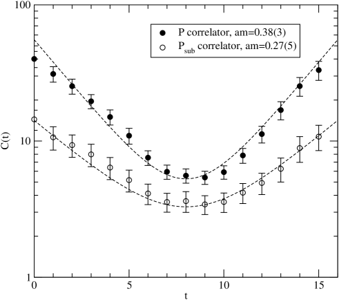
Figure 6.7: Pseudoscalar correlators P and P_sub from full and zero mode subtracted quark propagators at the smallest quark mass $ma=0.01$ on the $6^{3}\times 16$ lattice at $\beta=3.0$. The dashed lines are from correlated fits to the range $t\in[4,8]$.

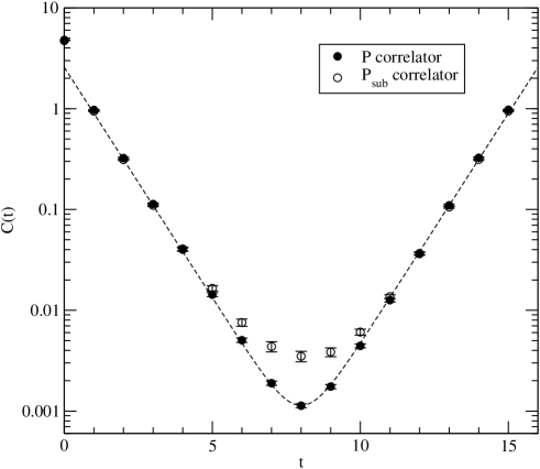
Figure 6.9: Pseudoscalar correlators P and P_sub from full and zero mode subtracted quark propagators at the largest quark mass $ma=0.32$ on the $6^{3}\times 16$ lattice at $\beta=3.0$.

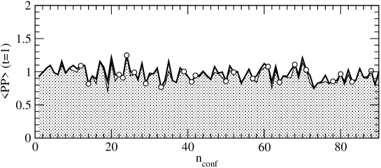
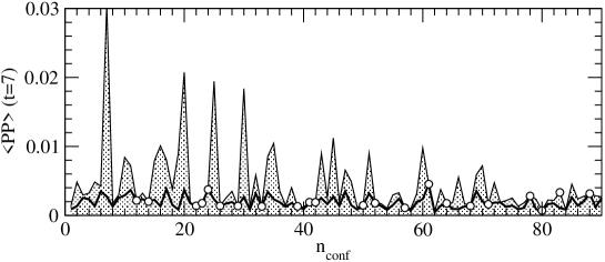
Figure 6.10: Monte Carlo time evolution of full (thick empty line) and zero mode subtracted (filled) pseudoscalar correlator at quark mass $am=0.32$. Shown are the correlators at times $t=1$ (top) and $t=7$ (bottom). Empty dots mark topologically trivial gauge configurations.

Figure 6.11: Three different methods of removing the quenched topological finite-volume artifacts in pion correlators. The lattice size is $6^{3}\times 16$, and the gauge coupling $\beta=3.0$. Within errors, all three methods lead to the same results at small quark mass and go to zero in the chiral limit $m\rightarrow 0$. The zero mode effects are no longer present. Compared are the P-S correlator, the ${\rm P_{sub}}$ correlator from zero mode subtracted quark propagators and the P correlator evaluated only on gauge configurations with topological charge $Q=0$. The last method is of course in general not allowed, as the remaining set of gauge configurations no longer follows the probability distribution given by the partition function of the quenched theory.

Chapter 7 The Light Hadron Spectrum with Fixed-Point Fermions

Since the first attempts in 1981 [122, 123], many lattice studies of the light hadron spectrum in quenched QCD have been performed, with quality increasing with time. The first systematic calculation was done in 1993 by the GF11 collaboration [124], but today’s benchmark is the CP-PACS calculation [125, 126] from 1998, which included a thorough examination of the chiral and continuum extrapolations and very high statistics. In their study, the most simple choice of actions was taken, namely the Wilson plaquette and fermion actions, and a full year of runs on the dedicated CP-PACS computer with a peak performance of 614 GFLOPS was necessary in order to obtain the quenched particle spectrum in a controlled manner. Because the cut-off effects for the Wilson action are known to be large, the simulation was performed at rather small lattice spacings in the range $a\approx 0.05$–$0.1$ fm. To avoid finite volume effects, the physical size was chosen to be 3 fm, which required to run on lattices of sizes up to $64^{3}\times 112$. The Monte Carlo average was taken from up to 800 independent gauge configurations. Their result is a physical particle spectrum with very small statistical errors, which are on the order of 1–2% for mesons and 2–3% for baryons, and with systematic errors from the extrapolations that are estimated to be even smaller. The calculated hadron masses agree qualitatively with the experimentally observed spectrum, but the mass values deviate by up to 11% or $7\sigma$, which is thought to be the error introduced by the quenched approximation.

A crucial part in the analysis of the CP-PACS data was the chiral extrapolation. The quark mass was pushed down to a value corresponding to $m_{\rm PS}/m_{\rm V}\approx 0.4$, which is very small for the Wilson action with its inherent chiral symmetry breaking, and only with the point at the lowest quark mass it was possible to resolve the non-analytic contributions predicted by quenched chiral perturbation theory (Q$\chi$PT) [127, 128]. It is however important to investigate whether including such Q$\chi$PT terms leads to significantly different mass values in the chiral limit than when using just low-order polynomial forms, as usually done in earlier works.

Exact or approximately chiral fermion actions allow to go to much smaller quark masses than the Wilson action. It is therefore possible to explore the chiral limit directly, to check the significance of the Q$\chi$PT terms and thus to increase the reliability of the hadron mass extrapolation to the physical quark mass. In this Chapter, we report the results of a spectroscopy calculation with the parametrized FP fermion action which probes deep into the chiral limit and also includes investigations of the scaling properties of the hadron masses and their finite-volume dependence. With a total amount of computer resources of about 20 GFLOPS$\times$years theoretical peak and an effective amount of about 6 GFLOPS$\times$years, this study in the framework of the BGR collaboration [129] by no means attempts to compete with the above mentioned high-statistics calculations. However, in addition to an independent test for spectroscopy simulations with a new formulation of the lattice QCD action, we get important information from the region of small quark masses, where non-chiral actions do not allow to perform simulations. Furthermore, this is one of the first spectroscopy studies with a chiral symmetric fermion action that examines cut-off effects.

Before we started this simulation, we carried out some tests for spectroscopy with the FP action on a smaller scale, the results of which are published in [4, 2]. The lattice parameters of these tests are listed for completeness in Table 7.1.

$D$	$\beta$	$L_{s}^{3}\times L_{t}$	$a(r_{0})$	$La(r_{0})$	# confs.	# masses	$m_{\rm PS}/m_{\rm V}$
FP	3.0	$6^{3}\times 16$	0.16 fm	0.9 fm	100	10	0.35–0.8
FP	3.0	$8^{3}\times 24$	0.16 fm	1.3 fm	100	13	0.3–0.85
FP	3.0	$9^{3}\times 24$	0.16 fm	1.4 fm	70	12	0.3–0.85
ov3	3.0	$9^{3}\times 24$	0.16 fm	1.4 fm	28	10	0.27–0.85
ov3	3.2	$9^{3}\times 24$	0.13 fm	1.2 fm	32	10	0.24–0.89

Table 7.1: Parameters of exploratory spectroscopy simulations with the FP and overlap-improved (ov3) FP Dirac operator [4, 2].

$D$	$\beta$	$L_{s}^{3}\times L_{t}$	$a(r_{0})$	$La(r_{0})$	# confs.	$m_{\rm PS}/m_{\rm V}$	# iters.
FP	3.0	$8^{3}\times 24$	0.16 fm	1.3 fm	200	0.3–0.88	250(39)
FP	3.0	$12^{3}\times 24$	0.16 fm	1.9 fm	200	0.3–0.88	360(55)
ov3	3.0	$12^{3}\times 24$	0.16 fm	1.9 fm	100	0.21–0.88	618(61)
FP	3.0	$16^{3}\times 32$	0.16 fm	2.5 fm	200	0.28–0.88	478(74)
FP	3.4	$12^{3}\times 24$	0.10 fm	1.3 fm	200	0.34–0.89	306(37)
FP	3.7	$16^{3}\times 32$	0.08 fm	1.3 fm	100	0.34–0.89	469(52)

Table 7.2: Parameters of the spectroscopy simulation described in this work. The $12^{3}\times 24$ gauge configurations at $\beta=3.0$ are the same for the calculations with the FP and overlap-improved (ov3) FP Dirac operator. The last column shows the average number of iterations required for the inversion of $D$.

7.1 Simulation Parameters

For generating the gauge configurations, we use the parametrized isotropic Fixed-Point gluon action from [29]. While this action is relatively expensive compared to the Wilson action, generating the gauge configurations was a comparably small effort in terms of computer time in the context of this work, and therefore we could afford using a FP action also for the gluon sector. It was shown in [29] that the FP gauge action has small scaling violations in gluonic quantities and that it reproduces topological properties well. With this gauge action, we produced a set of configurations at various lattice sizes and gauge couplings as shown in Table 7.2, where we also list the lattice spacing determined from the Sommer scale $r_{0}\approx 0.5$ fm for the different values of the gauge coupling. This combination of parameters was chosen to allow for a scaling analysis at small physical spatial lattice size $L_{s}\approx 1.3$ fm and a finite-volume analysis at gauge coupling $\beta=3.0$. The largest lattice at $\beta=3.0$ has a physical volume large enough to accommodate hadrons with negligible finite-volume effects. While this value of the gauge coupling is quite far away from the continuum, we expect to get on this lattice precise numbers for hadron masses which can serve as good estimates for the continuum values, because as we will show, the FP action has small scaling violations. We use alternating Metropolis and pseudo-overrelaxation sweeps over the lattice, with 2000 sweeps for thermalization and 500 sweeps to separate between different configurations. The number of separation sweeps is a worst-case estimate based on measurements of autocorrelation times for simple gluonic operators [131]. The configurations are then smeared with the RG inspired two-level hypercubic smearing described in [6] and fixed to Coulomb gauge with the algorithm presented in Appendix A. We use periodic boundary conditions for both the gauge and fermion fields.

For the fermion action, we take the parametrized FP Dirac operator from Chapter 3, except for one lattice, where the overlap-improved FP Dirac operator from Chapter 4 is used. With the third-order overlap expansion, we decrease the small residual chiral symmetry breaking of the parametrization even further and are able to check what effect the overlap construction has on the mass spectrum. The quark masses cover a very large range, with the smallest value, where $m_{\rm PS}/m_{\rm V}\approx 0.21$, lying close to the physical point. This provides us with meaningful data for chiral fits and allows for a thorough examination of the chiral limit. To enhance the signal for the hadron correlators, we use Gaussian smeared sources located at the center of timeslice $t=0$. The source extension parameter $\gamma$ in Eq. (5.26) is chosen to correspond to a source size of $\sim 0.5$ fm. We use point sinks and project to zero momentum by summing over all spatial sink locations. Quark propagators are calculated with the multi-mass BiCGstab inversion algorithm [132] (see also Appendix B.3). Source vectors are normalized to 1, and as a stopping criterion, we require the residual to be smaller than some threshold $|r|\leq\sigma$.

Due to the fact that a multi-mass solver inverts the Dirac matrix at all quark masses simultaneously, the result of the inversion at larger masses is more accurate than at the smallest one, where the condition number of the Dirac matrix is worst. The value of $\sigma$ therefore determines the accuracy of the quark propagators at the smallest quark mass, while the propagators at larger masses are calculated to much higher precision, as shown in Fig. 7.1. In order to demonstrate that the error from the truncation of the inversion algorithm is much smaller than the statistical error from the Monte Carlo estimate of the hadron correlators, we show in Table 7.3 the dependence of pseudoscalar and vector meson correlators on the stopping criterion. Based on this data, we choose a precision of $\sigma=10^{-6}$ for the inversion of the Dirac operator, which leads to an error from the truncation of the iterative inversion algorithm that is negligible compared to the statistical error. At our intermediate and larger quark masses, the quark propagator is almost calculated to machine precision. The average number of iterations needed for the inversion on the various lattices is also given in Table 7.2.

To check whether the computed hadron propagators are statistically independent, we calculate the statistical error of effective meson masses in dependence of the number of configurations $N$ used for the Monte Carlo average. If the gauge configurations are independent, the bootstrap error is proportional to $1/\sqrt{N}$. In Fig. 7.2 we plot the error in effective pseudoscalar meson masses at various values of $t$ on the $12^{3}\times 24$ lattice at $\beta=3.4$. As we can see, the curves nicely agree with the expected $1/\sqrt{N}$ behavior. For a second check, we collect bins of $N_{\rm bin}$ successive propagators, take the average of each bin and calculate the statistical error in effective masses from the $N/N_{\rm bin}$ binned propagators. The resulting bootstrap error, plotted in Fig 7.3, turns out to be independent of the bin size $N_{\rm bin}$. These two observations confirm that the number of separation sweeps used in the generation of the gauge configurations is sufficient to ensure statistical independence.

Figure 7.1: Residual for quark propagator inversion at different quark masses. The tolerance of the multi-mass solver is set to $\sigma=10^{-6}$.

correlator	$am_{q}$	$\Delta^{\rm rel}(\sigma=10^{-8})$	$\Delta^{\rm rel}(\sigma=10^{-6}$)	$\Delta^{\rm rel}x(\sigma=10^{-4}$)
PS	0.016	$3\cdot 10^{-8}$	$8\cdot 10^{-6}$	$0.001$
V	0.016	$4\cdot 10^{-7}$	$7\cdot 10^{-5}$	$0.014$
PS	0.04	$5\cdot 10^{-14}$	$7\cdot 10^{-11}$	$4\cdot 10^{-7}$
V	0.04	$2\cdot 10^{-12}$	$1\cdot 10^{-9}$	$4\cdot 10^{-6}$

Table 7.3: Relative error $\Delta^{\rm rel}(\sigma)=(C(\sigma)-C_{\rm exact})/C_{\rm exact}$ of meson correlators $C(t=8)$ on one $9^{3}\times 24$ gauge configuration at $\beta=3.0$. The dependence on the tolerance $\sigma$ of the residual in the quark propagator inversion is shown. The ’exact’ result $C_{\rm exact}$ is calculated with tolerance $\sigma=10^{-12}$. For comparison, the statistical error of PS and V correlators at $t=8$ is always larger than 1 % in our simulations.

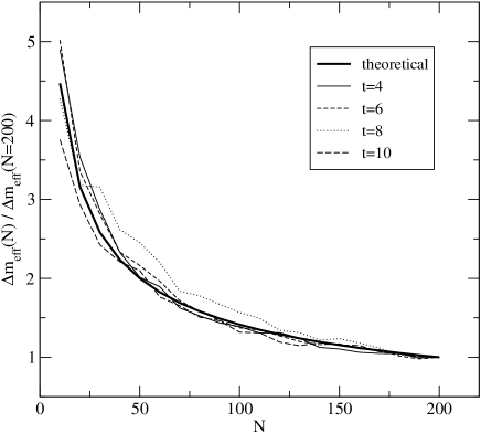
Figure 7.2: Dependence of the statistical error in effective pseudoscalar meson masses on the number of gauge configurations $N$. The data is taken from the $\beta=3.40$ configurations on the $12^{3}\times 24$ lattice, and the quark mass is $am_{q}=0.10$. The curves are normalized to 1 at $N=200$.

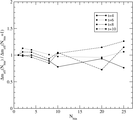
Figure 7.3: Dependence of the statistical error in effective pion masses on the bin size $N_{\rm bin}$. The data is taken from 200 $\beta=3.40$ configurations on the $12^{3}\times 24$ lattice, and the quark mass is $am_{q}=0.10$. The curves are normalized to 1 at $N_{\rm bin}=1$.

We list our hadron mass results on the different lattices for the pseudoscalar and vector mesons and the octet and decuplet baryons from quarks with degenerate masses, together with the temporal fit range and the resulting value of $\chi^{2}/df$ for the fit, in Appendix D.1. To account for a possibly biased determination of the fitted masses we apply bootstrap bias correction, as defined in Eq. (5.40), to the fit results.

Fig. 7.4 gives an overview of the masses of the hadrons in dependence of the quark mass on the various lattices in our simulation. We remind the reader that due to the use of a multi-mass solver, the results at different quark masses are highly correlated. This fact has to be taken into account when interpreting the data presented in this chapter.

The following analysis of our spectroscopy runs has to be considered preliminary. We try to give in this work some first answers to the main questions that arise from the use of such a new chiral action for the determination of the hadron spectrum.

7.2 Zero Mode Effects

In Chapter 6, we showed that divergent zero mode contributions appear in pion propagators and examined these quenching artifacts and possible ways to remove them on a small lattice volume. We concluded that it seems sensible to work with different correlators at different quark masses. We return to this issue here and present the zero modes effects seen in the data of our spectroscopy simulation.

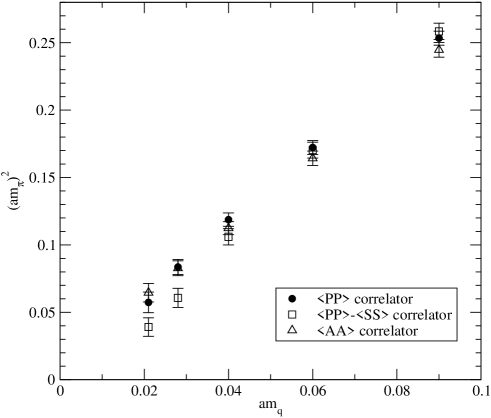
Figure 7.6: Pion mass squared versus bare quark mass for the three pion correlators on lattice size $8^{3}\times 24$ with $\beta=3.0$ for $D^{\rm FP}$.

In Figs. 7.5–7.10 the Monte Carlo history of the three correlators P, A, and P-S and the resulting pseudoscalar meson masses are shown on the three different lattice volumes at gauge coupling $\beta=3.0$. The values of the correlators in the Monte Carlo time plots are taken from timeslice $t=8$ and quark mass $am_{q}=0.021$. As expected, in the case of the smallest lattice of size $8^{3}\times 24$ in Fig. 7.5, there are a few very prominent peaks in the P correlator which dominate the gauge average completely. Also the A correlator is dominated by these peaks, but to a somewhat smaller extent. In contrast to these heavily contaminated correlators, many more configurations contribute to the average of the P-S correlator. Considering the absolute scale, it is obvious that the zero mode contributions, which are present in both the pseudoscalar and scalar correlators, are cancelled to a large extent in the difference. The resulting pseudoscalar meson masses from these three correlators, plotted in Fig. 7.6, differ significantly at the smallest quark masses.

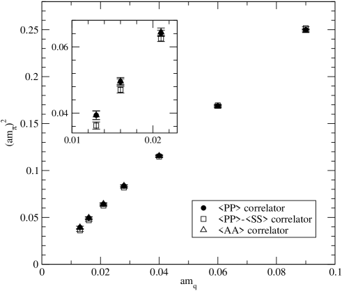
Figure 7.10: Pion mass squared versus bare quark mass for the three pion correlators on lattice size $16^{3}\times 32$ with $\beta=3.0$ for $D^{\rm FP}$.

On the lattice with intermediate size $12^{3}\times 24$, the same effects in the Monte Carlo history of the correlators can be observed in Fig 7.7, but they are much less pronounced. Again, the largest peaks in the P correlator are cancelled in the P-S correlator. The masses in Fig. 7.8 agree much better, but still a systematic deviation is visible. On the largest lattice (Fig. 7.9), all three correlators show a fairly smooth behavior. The mass of the pseudoscalar meson (Fig. 7.10) depends only very little on the choice of correlator. We summarize this analysis by listing the relative difference in meson masses from the P and P-S correlators in dependence of the lattice volume and quark mass in Table 7.4, a quantity which serves as a crude estimate for the size of the zero mode effects.

$8^{3}\times 24$, $\beta=3.0$		$12^{3}\times 24$, $\beta=3.0$		$16^{3}\times 32$, $\beta=3.0$
$V\approx 7$ fm4		$V\approx 24$ fm4		$V\approx 76$ fm4
$m_{\rm PS}/m_{\rm V}$	$\Delta m_{\rm PS}$	$m_{\rm PS}/m_{\rm V}$	$\Delta m_{\rm PS}$	$m_{\rm PS}/m_{\rm V}$	$\Delta m_{\rm PS}$
0.28	29(13)%	0.30	14(5)%	0.28	4(2)%
0.35	17(8)%	0.35	6(3)%	0.31	3(1)%
0.48	6(4)%	0.41	3(2)%	0.36	1(1)%

Table 7.4: Estimated size of zero mode effects in pseudoscalar meson masses from their relative difference when determined from the P, A and P-S correlators.

We conclude from these observations that on our largest lattice with spatial extension $L_{s}\approx 2.5$ fm, the zero mode contributions are sufficiently small to allow for a reliable determination of the mass in the pseudoscalar channel and the quantitative examination of its chiral limit. Only at the two smallest quark masses, the results from the different correlators do not agree within the (already small) statistical errors. On the smaller lattices, the uncertainty grows rapidly with decreasing quark mass, and therefore it becomes increasingly hard to keep the zero mode effects under control. We will in the following adopt the strategy suggested in Chapter 6 and construct the pseudoscalar meson from the P-S correlator at small and the P correlator at large quark mass. At the smaller lattice volumes, this introduces a systematic uncertainty at the few smallest quark masses, where we can not control how well the subtraction in the meson correlators works. But as our results will show, this strategy turns out to be successful in our simulations.

7.3 Chiral Extrapolations and Quenched Chiral Logarithms

With the approximately chiral Fixed-Point fermion action, we are in a position to study the chiral limit of hadron masses in detail. After measuring the residual additive quark mass renormalization, we examine in this section the quark mass dependence of the pseudoscalar meson mass and check for the presence of quenched chiral logarithms. On our largest lattice, we also calculate the resulting spectrum of $K$, $K^{*}$ and $\phi$ mesons and $N$, $\Delta$ and $\Omega$ baryons after extrapolating the measured data for the degenerate hadrons to the physical values of the average up and down quark and the strange quark mass, respectively.

7.3.1 Residual Quark Mass

We first determine the residual additive quark mass renormalization introduced by the parametrization of the Fixed-Point Dirac operator. From the axial Ward identity (AWI), the quark mass $m_{q}^{\rm AWI}$ is given by the large $t$ limit of

$$Z_{m}m_{q}^{\rm AWI}(t)=\frac{1}{2}\frac{Z_{A}\sum_{\vec{x}}\langle\partial_{4}A_{4}(\vec{x},t)C(0)\rangle}{Z_{P}\sum_{\vec{x}}\langle P(\vec{x},t)C(0)\rangle},$$ (7.1)

where $C(0)$ is a source operator with the quantum numbers of the pion and $A_{4}(\vec{x},t)$ and $P(\vec{x},t)$ are the local fourth component axial vector and pseudoscalar currents. As seen in Fig. 7.11, the ratio of the two correlators in Eq. (7.1) is flat already at small $t$ and can easily be fitted to a constant also at very small quark masses. The unrenormalized AWI quark masses $m_{q}^{\rm AWI}$ extracted from our data are listed in Appendix D.2. Although we do not know the renormalization factors $Z_{m}$, $Z_{S}$ and $Z_{A}$, the residual quark mass can be determined from the value of the bare quark mass $m_{q}$ where the AWI quark mass vanishes, by linearly extrapolating the measured ratio of correlators to zero.

The resulting values of $m_{\rm res}^{\rm(AWI)}=m_{q}(m_{q}^{\rm AWI}=0)$ from a linear fit to the six smallest masses on each lattice are shown in Table 7.5. At $\beta=3.0$, the residual mass for both the parametrized and the overlap-improved FP Dirac operator is very close to zero, whereas at larger $\beta$, its value is clearly non-zero. This is not surprising, since we have optimized the parametrization to $\beta\approx 3.0$ by choosing a set of gauge configurations with $2.7<\beta<3.4$ to fit the FP relation. While the fluctuations of the smallest eigenvalues of the Dirac operator decrease with increasing $\beta$, the central value is slightly shifted away from zero, leading to a non-vanishing value of $m_{\rm res}^{\rm(AWI)}$ at larger $\beta$. Obviously the fluctuation polynomials in the parametrized FP Dirac operator do not fully absorb this $\beta$-dependence of the eigenvalue spectrum.

$\beta$	Dirac operator	$m_{\rm res}^{\rm(AWI)}$
3.0	parametrized FP	-0.0006(4)
3.0	overlap-improved FP	-0.0006(1)
3.4	parametrized FP	-0.0180(4)
3.7	parametrized FP	-0.0194(2)

Table 7.5: The residual quark mass determined from the axial Ward identity.

7.3.2 The Quenched Chiral Log Parameter $\delta$

Chiral perturbation theory ($\chi$PT) [133] allows to predict the quark mass dependence of hadrons. In particular the pion, taking the role of the Goldstone boson of spontaneously broken chiral symmetry, should be massless in the chiral limit, and to lowest order in $\chi$PT, it depends linearly on the quark mass. Taking into account the quenched approximation, additional logarithmic terms appear: Quenched chiral perturbation theory predicts the following dependence of the pseudoscalar meson mass $m_{\rm PS}$ on the two constituent quark masses $m_{1}$ and $m_{2}$ [127, 126]:

$$m_{\rm PS}^{2}=A(m_{1}+m_{2})\left[1-\delta\left(\ln\frac{2Am_{1}}{\Lambda_{\chi}^{2}}+\frac{m_{2}}{m_{2}-m_{1}}\ln\frac{m_{2}}{m_{1}}\right)\right]+B(m_{1}+m_{2})^{2}\\ +{\mathcal{O}}(m_{q}^{3}),$$ (7.2)

where $\Lambda_{\chi}$ is a Q$\chi$PT scale and of order 1 GeV. The term proportional to $\delta$ is divergent in the chiral limit and is only present due to quenching. In the case of degenerate quark masses, the divergence can be absorbed into a redefinition of the quark mass by resummation of the leading logarithms [128]. This yields a power form

$$m_{\rm PS}^{2}\propto m_{q}^{\frac{1}{1+\delta}},$$ (7.3)

for the pseudoscalar mass. To leading order in a $1/N_{c}$-expansion, the value of the parameter $\delta$ is given by [126]

$$\delta=\frac{m_{\eta^{\prime}}^{2}+m_{\eta}^{2}-2m_{K}^{2}}{48\pi^{2}f_{\pi}^{2}}\approx 0.18,$$ (7.4)

where the pion decay constant is normalized such that $f_{\pi}=93$ MeV.

CP-PACS has estimated a value of $\delta=0.10(2)$ from their analysis of pseudoscalar mesons with non-degenerate quarks and $\delta=0.09(3)$ from a fit of Eq. (7.2) to pseudoscalar mesons with degenerate quarks, where the scale was varied in the range $0.6$ GeV$<\Lambda_{\chi}<1.4$ GeV. The drawback of their data is the use of the Wilson action with its explicit breaking of chiral symmetry, which allows to cover only a limited range of quark masses because of the appearance of exceptional configurations. Recently a technique has been proposed for the Wilson action to shift the would-be zero modes, that fluctuate far along the positive real axis, back to zero [134]. This pole-shifting procedure amounts to a modification of the quenched theory and prevents exceptional configurations, thus allowing to go almost down to the physical pion mass even with Wilson fermions. However, one has to assume that the most important effect of explicit chiral symmetry breaking in the Wilson action is the resulting fluctuation of the zero modes on the real axis. The chiral properties are not improved for other parts of the spectrum, and therefore it is not clear how much such a punctual modification helps. In [135], the chiral log parameter $\delta$ has been determined in various ways, amongst others also from the pseudoscalar meson mass, with the pole-shifted Wilson action and similar simulation parameters like we use here. The quoted value averaged over the different determinations is $\delta=0.065(13)$, which is a factor of three smaller than the theoretical estimate, but fairly consistent with the CP-PACS result.

It would obviously be interesting to determine the value of $\delta$ with a chiral symmetric action, which is free of problems related to exceptional configurations and does not only cure the explicit chiral symmetry breaking punctually. In [85, 80, 81], investigations of the chiral limit with the Wilson overlap action were performed, and varying values of $\delta$ were found, with a tendency towards larger values than what was obtained with non-chiral actions. With our data, we are not only able to quite precisely determine the value of $\delta$ from the pseudoscalar meson mass, but we can also compare the results for the approximately chiral parametrized FP and the overlap-improved Dirac operator, providing two at least partially independent results with chiral actions.

First we examine the mass of the pseudoscalar meson with degenerate quarks, calculated from the P and P-S correlators on various lattices at $\beta=3.0$. We fit the masses to the polynomial forms

$$(am_{\rm PS})^{2} = 2Aa^{2}(m_{q}+m_{\rm res})+4Ba^{3}(m_{q}+m_{\rm res})^{2},$$ (7.5)

$$(am_{\rm PS})^{2} = 2Aa^{2}(m_{q}+m_{\rm res})+4Ba^{3}(m_{q}+m_{\rm res})^{2}$$ (7.6)

$$+8Ca^{4}(m_{q}+m_{\rm res})^{3},$$

and to the forms inspired by quenched chiral perturbation theory

$$(am_{\rm PS})^{2} = 2Aa^{2}(m_{q}+m_{\rm res})\left[1-\delta\left(\ln\frac{2Aa^{2}(m_{q}+m_{\rm res})}{a^{2}\Lambda_{\chi}^{2}}+1\right)\right]$$ (7.7)

$$+4Ba^{3}(m_{q}+m_{\rm res})^{2},$$

$$(am_{\rm PS})^{2} = 2Aa^{2}(m_{q}+m_{\rm res})^{\frac{1}{1+\delta}},$$ (7.8)

$$(am_{\rm PS})^{2} = 2Aa^{2}(m_{q}+m_{\rm res})^{\frac{1}{1+\delta}}+4Ba^{3}(m_{q}+m_{\rm res})^{2},$$ (7.9)

allowing for a residual additive quark mass renormalization $am_{\rm res}$. The resulting fit parameters for all three lattices are listed in Table 7.6. The errors are determined by bootstrap resampling, calculating on each of the 500 bootstrap samples the meson masses from a correlated fit and using these for the chiral fit.

The most reliable results are obtained on the largest lattice. There it is obvious that a quadratic fit with a value of $\chi^{2}/df=11.5$ misses the clear negative curvature at small quark masses in our data. Also a cubic fit with $\chi^{2}/df=2.9$ can not account for this curvature well. In contrast, the various Q$\chi$PT fits agree perfectly with our data, with $\chi^{2}/df\approx 0.5$. In Fig. 7.12 we compare the logarithmic fit with $\Lambda_{\chi}=1$ GeV and the quadratic fit, showing the clear discrepancy when the quenched chiral log is neglected. In Table 7.7 we demonstrate that the results for $\delta$ on the largest lattice do not differ significantly when choosing one single correlator P, A or P-S instead of extracting the pseudoscalar masses from the P and P-S correlators at different quark mass according to our proposition.

On the $12\times 24$ lattice, the results for $\delta$ with the parametrized FP Dirac operator agree very well with those at $16^{3}\times 32$, with somewhat larger errors. Also with the overlap-improved operator, we get consistent values, but the errors are then even larger due to the smaller statistics. We compare our values of $\delta$ from the degenerate mesons with those from [81] in Table 7.8. From the results of the fits to the logarithmic form (7.7) on the largest lattice, we estimate a value of $\delta=0.17(3)$, where the error mostly comes from the unknown scale $\Lambda_{\chi}$.

$16^{3}\times 32$, $\beta=3.0$, parametrized FP
fit form	$am_{\rm res}$	$\delta$	$aA$	$aB$	$\chi^{2}$/df
quadratic (7.5)	0.0040(4)		1.22(1)	0.51(1)	11.5(2.0)
cubic (7.6), $C=0.55(4)$	0.0019(5)		1.35(2)	-0.02(5)	2.9(8)
log (7.7), $\Lambda_{\chi}\simeq 0.6$ GeV	-0.0018(6)	0.143(9)	1.46(3)	0.94(3)	0.6(3)
log (7.7), $\Lambda_{\chi}\simeq 0.8$ GeV	-0.0017(5)	0.157(10)	1.32(1)	0.94(3)	0.5(2)
log (7.7), $\Lambda_{\chi}\simeq 1.0$ GeV	-0.0017(6)	0.172(12)	1.21(1)	0.94(3)	0.5(3)
log (7.7), $\Lambda_{\chi}\simeq 1.2$ GeV	-0.0017(6)	0.186(15)	1.12(1)	0.94(3)	0.5(2)
log (7.7), $\Lambda_{\chi}\simeq 1.4$ GeV	-0.0017(6)	0.200(17)	1.04(2)	0.94(3)	0.5(2)
power (7.8), 5 masses	-0.0039(9)	0.229(40)	0.86(7)		0.8(5)
power (7.8), 6 masses	-0.0024(9)	0.132(30)	1.05(6)		0.9(4)
power+quadr. (7.9)	-0.0026(7)	0.194(16)	0.86(2)	0.9(2)	0.4(2)

$12^{3}\times 24$, $\beta=3.0$, parametrized FP
fit form	$am_{\rm res}$	$\delta$	$aA$	$aB$	$\chi^{2}$/df
quadratic (7.5)	0.0043(11)		1.21(2)	0.53(2)	4.7(1.4)
cubic (7.6), $C=0.53(8)$	0.0009(14)		1.35(4)	0.0(1)	1.0(4)
log (7.7), $\Lambda_{\chi}\simeq 0.8$ GeV	-0.0035(16)	0.165(18)	1.34(3)	0.95(5)	0.2(1)
log (7.7), $\Lambda_{\chi}\simeq 1.0$ GeV	-0.0035(15)	0.181(21)	1.22(2)	0.95(4)	0.2(2)
log (7.7), $\Lambda_{\chi}\simeq 1.2$ GeV	-0.0035(15)	0.196(25)	1.13(1)	0.95(4)	0.2(2)
power (7.8), 5 masses	-0.0050(15)	0.164(72)	1.0(1)		0.1(1)
power (7.8), 6 masses	-0.0029(17)	0.079(26)	1.19(5)		0.3(4)
power+quadr. (7.9)	-0.0045(17)	0.209(28)	0.86(3)	0.87(4)	0.1(1)

$12^{3}\times 24$, $\beta=3.0$, overlap-improved
fit form	$am_{\rm res}$	$\delta$	$aA$	$aB$	$\chi^{2}$/df
quadratic (7.5)	0.0036(20)		1.36(3)	0.52(3)	1.3(8)
cubic (7.6), $C=0.55(17)$	0.0011(20)		1.51(6)	0.0(2)	0.4(4)
log (7.7), $\Lambda_{\chi}\simeq 0.8$ GeV	-0.0020(22)	0.141(35)	1.50(5)	0.93(10)	0.1(2)
log (7.7), $\Lambda_{\chi}\simeq 1.0$ GeV	-0.0021(23)	0.153(45)	1.39(3)	0.94(12)	0.1(2)
log (7.7), $\Lambda_{\chi}\simeq 1.2$ GeV	-0.0020(23)	0.163(51)	1.30(3)	0.93(12)	0.1(2)
power (7.8), 6 masses	-0.0039(24)	0.21(14)	1.0(3)		0.0(1)
power (7.8), 7 masses	-0.0037(23)	0.19(9)	1.0(2)		0.0(1)
power+quadr. (7.9)	-0.0020(24)	0.162(50)	1.30(3)	0.93(11)	0.1(2)

Table 7.6: Fit parameters for different forms of the chiral fit to the squared pseudoscalar meson mass on $\beta=3.0$ lattices. The power form (7.8) was fitted only to the few smallest masses, where the quadratic dependence is negligible.

$16^{3}\times 32$, $\beta=3.0$, parametrized FP
correlator	$am_{\rm res}$	$\delta$	$aA$	$aB$	$\chi^{2}$/df
P	-0.0004(6)	0.158(13)	1.19(1)	0.91(3)	0.4(3)
A	-0.0002(6)	0.158(13)	1.18(1)	0.92(3)	0.4(2)
P-S	-0.0018(6)	0.169(15)	1.22(1)	0.93(4)	0.4(2)
P-S at $am_{q}\leq 0.04$, P else	-0.0017(6)	0.172(12)	1.21(1)	0.94(3)	0.5(3)

Table 7.7: Fit parameters for logarithmic fit with $\Lambda_{\chi}=1$ GeV to the squared pseudoscalar meson mass on the largest lattice in dependence of the chosen correlators.

$\Lambda_{\chi}$	$\delta$ (Dong et al. [81])	$\delta$ (this work)
0.6 GeV	0.23(7)	0.143(9)
0.8 GeV	0.28(11)	0.157(10)
1.0 GeV	0.34(17)	0.172(12)

Table 7.8: The quenched chiral log parameter $\delta$ from a logarithmic Q$\chi$PT fit (7.7) to the pseudoscalar meson mass.

The quenched chiral log parameter $\delta$ can also be determined from an analysis of the non-degenerate pseudoscalar meson masses. The two quantities

$$x=2+\frac{m_{1}+m_{2}}{m_{1}-m_{2}}\ln\left(\frac{m_{2}}{m_{1}}\right),$$ (7.10)

$$y=\frac{2m_{1}}{m_{1}+m_{2}}\frac{m_{\rm PS,12}^{2}}{m_{\rm PS,11}^{2}}\cdot\frac{2m_{2}}{m_{1}+m_{2}}\frac{m_{\rm PS,12}^{2}}{m_{\rm PS,22}^{2}},$$ (7.11)

are related by $y=1+\delta x+{\mathcal{O}}(m^{2})$, and the terms proportional to $B(m_{1}+m_{2})$ in Eq. (7.2) cancel [126]. To avoid problems with the residual additive renormalization, we use the axial Ward identity quark masses (7.1) as an input for $m_{1}$ and $m_{2}$. Fig. 7.13 shows our data for the non-degenerate pseudoscalar mesons from the P correlator on the largest lattice. Only the points from mesons with light enough quarks that the linear dependence of $y(x)$ remains valid are plotted. For mesons with two heavy quarks, we encountered a systematic deviation towards smaller values of $y$ for all $x$, therefore they are omitted here. The slope of $y(x)$, giving $\delta=0.170(20)$, is beautifully consistent with the above value for the equal quark mass case and with the theoretical prediction in Eq. (7.4).

Taking the intersection of the two determinations of the chiral log parameter from degenerate and non-degenerate pseudoscalar mesons, we obtain a value of $\delta=0.17(2)$. In Table 7.9, we compare this final result to previous determinations from other groups. While our result is measured at finite lattice spacing $a\approx 0.16$ fm, the $a$-dependence of $\delta$ appears to be small [126].

Group	year	Fermion action	$\delta$
JLQCD [136]	1996	staggered	0.05–0.10
CP-PACS [126]	1998	Wilson	0.10(2)
Bardeen et al. [135]	2000	pole-shifted Wilson	0.065(13)
Dong et al. [81, 80]	2001	Wilson overlap	0.23–0.48
This work	2002	Fixed-Point	0.17(2)

Table 7.9: Compilation of recent results for the quenched chiral log parameter $\delta$. Earlier results are reported in [137].

As a by-product of this analysis, we estimate a value of $am_{\rm res}^{\rm(PS)}=-0.002(2)$ for the residual quark mass of the parametrized FP Dirac operator, covering the various quenched fits to the pseudoscalar meson mass at $\beta=3.0$. This value agrees well with the residual mass determined from the axial Ward identity in Table 7.5, which is clearly not the case for $am_{\rm res}$ resulting from quadratic or cubic fits to $(am_{\rm PS})^{2}$. At the other values of the gauge coupling $\beta=3.4$ and $3.7$, we get larger values of $am_{\rm res}^{\rm(PS)}=-0.016(4)$ and $-0.012(7)$ respectively, in reasonable agreement with the results from the axial Ward identity. This coincidence confirms that measuring the pseudoscalar particle from the P correlator at large and the P-S correlator at small quark mass is a reasonable solution to avoid zero mode effects in the pseudoscalar mass.

7.3.3 Chiral Extrapolations for Vector Mesons and Baryons

For vector mesons and baryons, Q$\chi$PT predicts in the continuum limit [138, 139]

$$m(m_{\rm PS})=m_{0}+\delta C_{1/2}m_{\rm PS}+C_{1}m_{\rm PS}^{2}+C_{3/2}m_{\rm PS}^{3}+\dots,$$ (7.12)

where the $C_{i}$ are functions of the coefficients in the quenched chiral Lagrangian. Like in the formula for the pseudoscalar channel (7.2), the term proportional to $\delta$ appears only in the quenched theory, and according to Q$\chi$PT its coefficient $C_{1/2}$ is negative.

On our largest lattice, we perform chiral extrapolations for the vector meson and the octet and decuplet baryons both with and without the quenched term. The resulting fits are plotted in Fig 7.14. For the vector meson, there is some evidence for the presence of a term linear in $m_{\rm PS}$ with a negative coefficient, as expected from quenched chiral perturbation theory. The $\rho$ meson mass from the extrapolation to the physical quark mass, defined by $m_{\rm PS}/m_{\rm V}\approx 0.18$, is used to fix the lattice scale. For the fit including the quenched term, we get $a^{-1}=1104(32)$ MeV or $a=0.179(4)$ fm, while when setting $C_{1/2}=0$, we obtain $a^{-1}=1152(15)$ MeV or $a=0.171(2)$ fm. The two values do not completely coincide, showing that the functional form of the chiral extrapolation indeed can lead to different results. We use in the following the value obtained from the quenched fit, which includes in its error some of the uncertainty in the presence and size of the quenched term.

For the baryons, neither of the two functional forms is clearly favored by our data. The decuplet mass shows some upward curvature at the smallest quark masses, but the errors are quite large and do not cover the systematic uncertainty in choosing the fit range, which is increasingly difficult at small quark mass. What is however evident is the negative curvature in both baryon masses that gets absorbed by the $\mathcal{O}(m_{\rm PS}^{3})$ term, which is also present in ordinary chiral perturbation theory.

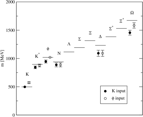
Figure 7.22: Part of the quenched light hadron spectrum at finite lattice spacing $a\approx 0.16$ fm. The quark mass $(m_{u}+m_{d})/2$ and the lattice spacing $a$ are determined from the $\pi$ and $\rho$ meson, and the strange quark mass $m_{s}$ is either fixed from the $K$ meson (filled symbols) or the $\phi$ meson (open symbols).

From a partial analysis of our data, we show in Fig. 7.22 the mass spectrum of hadrons with degenerate light quarks at $\beta=3.0$ and lattice size $16^{3}\times 32$. The familiar ambiguity from fixing the strange quark mass either with the $K$ or the $\phi$ meson is evident, and for both choices the meson hyperfine splitting turns out to be too small. The chiral extrapolation for the baryons, where the quenched term is included, leads to a nucleon mass which almost agrees with the experimental value, while the $\Delta$ and $\Omega$ baryon masses come out too small. However, since we are at finite lattice spacing, this discrepancy will not necessarily persist after a continuum extrapolation.

7.4 Physical Finite Size Effects

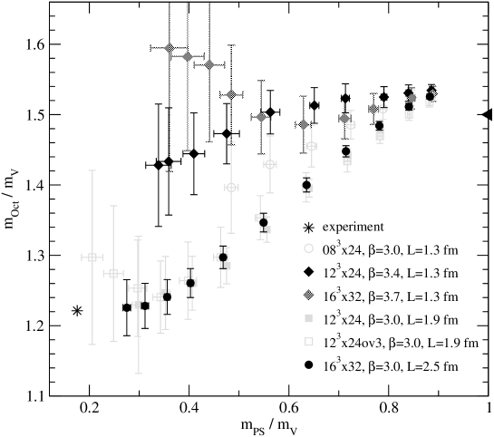
Figure 7.15: Our data compiled into an Edinburgh plot. Shown are the experimental point (star) and the theoretical prediction $m_{\rm Oct}/m_{\rm V}=1.5$ for the large mass limit (triangle). The three lattices with smallest physical volume show large finite-volume effects due to the increased mass of the octet baryon.

When the spatial lattice size is too small to accommodate the wave function of a hadron, its mass suffers from finite-size corrections. Results from quenched simulations show that for lattices larger than 2 fm, the finite volume effects are smaller than 2% [140]. As only our largest lattice with size $L_{s}\approx 2.5$ fm fulfills this requirement, we expect to see significant finite volume effects in our data on the smaller lattices. Plotting the ratio of octet baryon to vector meson masses in an Edinburgh plot (Fig. 7.15), we see that indeed on the lattices with spatial size $L_{s}\approx 1.3$ fm, this ratio stays more or less constant at $m_{\rm Oct}/m_{\rm V}\approx 1.5$ over the whole range of quark masses, thus being far too large in the chiral limit. However, already at lattice size $L_{s}\approx 1.9$ fm, the results do not differ anymore from those on the largest lattice within statistical errors.

We investigate the finite volume effects more closely in Fig. 7.16 by plotting the masses of all hadrons against the spatial lattice size. For the pseudoscalar meson, only the zero mode effects can be seen, leading to different results for different correlators. Also for the vector meson, there are no obvious finite-volume effects. The situation is different for the baryons: On the smallest lattice, the octet mass increases strongly, independent of the choice of correlator. The same happens with the decuplet mass, where the effect is slightly smaller.

We conclude from our data that at $\beta=3.0$, the finite-volume effects become comparable to our statistical errors already at $N_{s}=12$, corresponding to a spatial size of $L_{s}\approx 1.9$ fm. At $L_{s}\approx 1.3$ fm, the baryons are strongly affected by the small physical volume. The size of the largest lattice $L_{s}\approx 2.5$ fm is big enough to provide results which are not affected by finite-volume effects.

7.5 Scaling Properties

Let us turn to the investigation of the scaling behavior of the parametrized and overlap-improved FP fermion actions. A standard test for scaling violations of a given lattice action is to plot the vector meson mass, which is known to be particularly sensitive to cut-off effects, against the lattice spacing. Most groups use in this context the string tension to fix the scale. Except at $\beta=3.4$, we do not have a direct calculation of the string tension for our gauge action. Therefore we use the determination of $r_{0}/a$ from [130] instead, where the interpolating formula

$$\ln(a/r_{0})=-1.1539(18)-1.0932(68)(\beta-3)+0.132(11)(\beta-3)^{2},$$ (7.13)

is given and $r_{0}/\sqrt{\sigma}$ is measured, to set the scale from the string tension. Table 7.10 shows our measurements of the vector meson mass interpolated to $m_{\rm PS}/m_{\rm V}=0.7$ and the resulting value of $m_{V}/\sqrt{\sigma}$.

Our data is plotted in comparison with results from other fermion actions in Fig. 7.17. Wilson fermions have large $\mathcal{O}(a)$ and unimproved staggered fermions large $\mathcal{O}(a^{2})$ effects, which are clearly seen in the scaling of the vector meson mass. Fat links do not help to improve the situation. For the various types of clover actions shown, only small $\mathcal{O}(a^{2})$ effects remain, as it also seems to be the case for the FP action. While the parametrization of the FP action introduces cut-off effects to all orders, we do not see evidence for $\mathcal{O}(a)$ effects here.

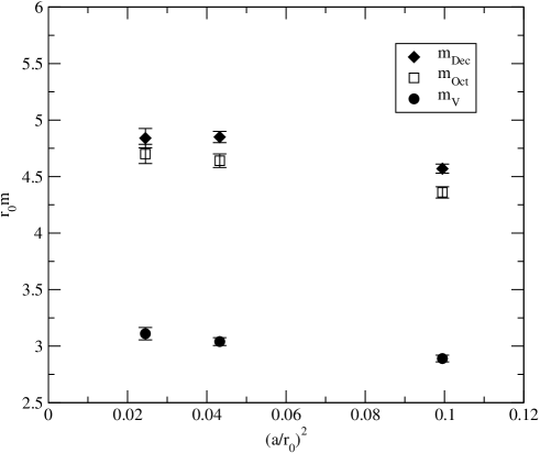
Figure 7.18: Scaling of hadrons on spatial lattice size $L_{s}\approx 1.3$ fm at $m_{\rm PS}/m_{\rm V}=0.78$ for the parametrized FP Dirac operator.

Because the conversion to the string tension introduces an additional error, it is not clear from this plot whether the scaling violations of the FP action are significant. We therefore determine the hadron masses in units of $r_{0}$ and plot them in Fig. 7.18. For all hadrons under consideration, the point at $\beta=3.0$ does not coincide within errors with the data at smaller lattice spacings. One has to take into account that the statistical error in $a/r_{0}$ does not fully cover the systematic uncertainty in determining the lattice scale at this $\beta$. Furthermore a scaling study in such a small physical volume encompasses the danger of substantial contributions from small differences in the lattice volume at the various values of the gauge coupling, because the volume dependence of the hadron masses at $L_{s}\approx 1.3$ is on the onset of getting strong [141]. Whether our data indicates the presence of small $\mathcal{O}(a^{2})$ cut-off effects in our parametrization of the FP fermion action or results from the determination of the Sommer scale $r_{0}$ and the related uncertainty in the lattice volume therefore needs further investigation.

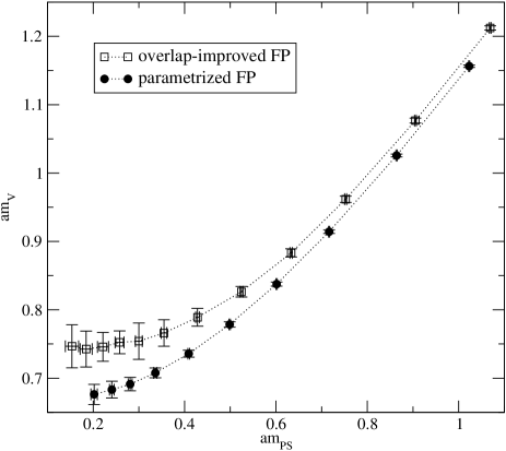
Figure 7.19: Comparison of vector meson mass for parametrized FP and overlap-improved FP Dirac operators.

A striking observation is that the vector meson mass turns out to be significantly larger for the overlap-improved Dirac operator than for the FP operator. We illustrate this by plotting $am_{\rm V}$ against $am_{\rm PS}$ in Fig. 7.19. Over the whole range of quark masses covered, a clear discrepancy is seen. This is to some extent surprising, since the overlap expansion is only carried out to third order and therefore one might expect that the properties of the input operator are only slightly changed. The discrepancy vanishes in the Edinburgh plot Fig. 7.15, where the results on the $12^{3}\times 24$ lattice agree for the FP and overlap-improved operators. The difference in the cut-off effects thus cancels in these mass ratios.

From our results we therefore find that the overlap-improvement changes the scaling behavior of the fermion action. In Fig. 7.17, the point for the overlap-improved operator at $\beta=3.0$ seems to agree with the continuum value obtained by extrapolating all the data to a single point at $a^{2}\sigma=0$, but this coincidence can be misleading due to a possible overall shift from the scale determination. To conclude whether the scaling violations are decreased or increased by the overlap, additional measurements with the overlap-improved FP Dirac operator at different values of $\beta$ are needed.

$\beta$	$N_{s}$	$D$	$a/r_{0}$	$a\sqrt{\sigma}$	$am_{q}$	$am_{\rm V}$	$m_{\rm V}/\sqrt{\sigma}$
3.7	16	FP	0.1565(16)	0.187(2)	0.076(3)	0.438(7)	2.34(4.4)
3.4	12	FP	0.2080(13)	0.248(3)	0.095(2)	0.568(6)	2.29(4)
3.0	8	FP	0.3154(16)	0.376(4)	0.123(2)	0.824(10)	2.19(4)
3.0	12	FP	0.3154(16)	0.376(4)	0.123(2)	0.827(4)	2.20(3)
3.0	16	FP	0.3154(16)	0.376(4)	0.123(2)	0.833(4)	2.21(3)
3.0	12	ov	0.3154(16)	0.376(4)	0.120(3)	0.871(9)	2.31(3)

Table 7.10: Data for the determination of the scaling violations in the vector meson mass at $m_{\rm PS}/m_{\rm V}=0.7$. To convert the scale to the string tension, we take the value of $r_{0}\sqrt{\sigma}=1.193(10)$ from [130], which was shown not to depend on $\beta$ significantly for the FP gauge action.

$\beta$	$N_{s}$	$am_{q}$	$am_{\rm V}$	$r_{0}m_{\rm V}$	$am_{\rm Oct}$	$r_{0}m_{\rm Oct}$	$am_{\rm Dec}$	$r_{0}m_{\rm Dec}$
3.7	16	0.105(2)	0.487(7)	3.11(5)	0.736(11)	4.70(9)	0.757(11)	4.84(9)
3.4	12	0.133(2)	0.632(6)	3.04(3)	0.965(10)	4.64(6)	1.009(9)	4.85(5)
3.0	8	0.179(3)	0.910(8)	2.89(3)	1.374(14)	4.36(5)	1.440(11)	4.57(4)

Table 7.11: Scaling of hadron masses in units of $r_{0}$ at $m_{\rm PS}/m_{\rm V}=0.78$ and lattice size $L_{s}\approx 1.3$ fm.

7.6 Hadron Dispersion Relations

Another quantity that measures the magnitude of discretization errors of a given action is the energy-momentum dispersion relation for hadrons $E(\vec{p})=m^{2}+\vec{p}\,^{2}$, or equivalently the squared speed of light

$$c^{2}(\vec{p}\,)=\frac{E^{2}(\vec{p}\,)-m^{2}}{\vec{p}\,^{2}},$$ (7.14)

which should be $c^{2}=1$ for all momenta according to the continuum dispersion relation. At large lattice spacings, unimproved lattice actions are known to suffer from substantial deviations from the continuum relation. Even for $\mathcal{O}(a)$-improved clover fermions, $c^{2}$ deviates by 20%–30% at $a=0.25$ fm and $p\approx 0.6$ GeV for pseudoscalar and vector mesons [142]. Our coarsest lattice spacing is $a=0.16$ fm, therefore we can not compare our results directly to this data. However, the energy-momentum dispersion relation for our pseudoscalar and vector mesons calculated with the parametrized FP Dirac operator on the lattice of size $16^{3}\times 32$, shown in Fig. 7.20, is consistent with $c^{2}=1$ over the whole range of momenta considered. The parametrization of the Fixed-Point Dirac operator therefore seems to conserve the classically perfect properties very well also for the dispersion relation.

It is interesting to check how the overlap-improved FP Dirac operator performs. We plot the squared speed of light at the smallest non-zero momentum on the $12^{3}\times 24$ lattice with $\beta=3.0$ in Fig. 7.21, and compare the results from the parametrized FP and the overlap-improved FP Dirac operator at the three largest quark masses. While the data from the FP operator again agrees with $c^{2}=1$ within errors for both mesons, the results from the overlap-improved operator are too large by 7(3)% for the pseudoscalar and 14(5)% for the vector meson. The overlap construction therefore seems to drive the hadronic dispersion relation of the FP operator away from the continuum form. The situation appears to be analogous to the case of the free Wilson operator, where the dispersion relation is also deteriorated by the overlap [143].

Figure 7.4: Compilation of hadron masses versus quark mass from the various lattices.

Figure 7.5: Monte Carlo time evolution of pion correlators at bare quark mass $am_{q}=0.021$ on lattice size $8^{3}\times 24$ with $\beta=3.0$ for $D^{\rm FP}$. Notice the large difference in the vertical scale of the P and P-S correlators.

Figure 7.7: Monte Carlo time evolution of pion correlators at bare quark mass $am_{q}=0.021$ on lattice size $12^{3}\times 24$ with $\beta=3.0$ for $D^{\rm FP}$.

Figure 7.8: Pion mass squared versus bare quark mass for the three pion correlators on lattice size $12^{3}\times 24$ with $\beta=3.0$ for $D^{\rm FP}$.

Figure 7.9: Monte Carlo time evolution of pion correlators at bare quark mass $am_{q}=0.021$ on lattice size $16^{3}\times 32$ with $\beta=3.0$ for $D^{\rm FP}$.

Figure 7.11: Unrenormalized quark mass $m_{q}^{\rm AWI}(t)$ from axial Ward identity (7.1) for bare quark masses $am_{q}=0.013$ and $am_{q}=0.028$ on $16^{3}\times 32$ at $\beta=3.0$.

Figure 7.12: Chiral fit to squared pseudoscalar meson mass with a quadratic function and the logarithmic form predicted by Q$\chi$PT with $\Lambda_{\chi}\simeq 1$ GeV, giving $\delta=0.17(1)$.

Figure 7.13: The quenched chiral log parameter $\delta$ from cross ratios (7.10), (7.11) of non-degenerate pseudoscalar meson masses. The solid line is a least-squares fit, where the slope gives $\delta=0.17$. The dashed lines correspond to $\delta=0.15$ and $\delta=0.19$, respectively.

Figure 7.14: Chiral extrapolations of vector meson and baryons on the $16\times 32$ lattice at $\beta=3.0$. The solid line is a fit without and the dashed line a fit including the quenched term in Eq. (7.12). The inset shows the resulting physical $\rho$, $N$ and $\Delta$ masses at the average up and down quark mass.

Figure 7.16: Finite volume effects in meson and baryon masses at $\beta=3.0$. The quark masses are from top to bottom $am_{q}=0.25$, 0.18, 0.13, 0.09 and for the mesons also $am_{q}=0.04$. For the pseudoscalar meson, masses from the A (open symbols) and P (filled) correlators are shown. For the baryons, full symbols are from the N and D and open symbols from the N0 and D0 correlators.

Figure 7.17: Scaling of the vector meson mass. Compared with the FP action is data from Wilson, staggered and various variants of clover actions. Filled and open boxes are data from this work. Crosses (Wilson) and stars (staggered) are from the compilation of Sharpe [144], open diamonds (NP clover) are from [145] and the fat link data and the open circles (Wilson) are from [146]. The rightmost point for the FP action is from a larger physical lattice size (with $N_{s}=16$) than the others, as there is no significant volume dependence seen in the data in Table 7.10.

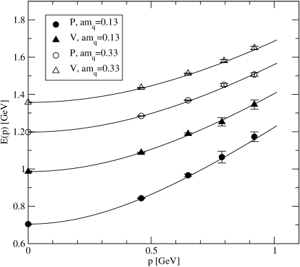
Figure 7.20: Energy-momentum dispersion relation $E(\vec{p})$ for pseudoscalar and vector mesons on the $16^{3}\times 32$ lattice with $\beta=3.0$. The solid lines show the continuum value with $E(0)$ given by the measured mass.

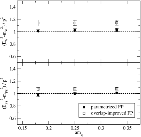
Figure 7.21: Comparison of squared speed of light $c^{2}$ from meson dispersion relations at the smallest non-zero momentum for parametrized FP and overlap-improved Dirac operators on the $12^{3}\times 24$ lattice with $\beta=3.0$.

Chapter 8 Conclusions and Prospects

After the beautiful properties of classically perfect Fixed-Point actions have been verified in various models, and recently a sophisticated FP $SU(3)$ gauge action has been parametrized and successfully tested, we have constructed in this work and in a parallel thesis a FP fermion action for lattice QCD. In this thesis it is applied to calculations of the quenched light hadron spectrum.

Properties of Fixed-Point Fermions

We find that the parametrization of FP fermions in QCD is a feasible task. The resulting Dirac operator is rather complex, including the full Clifford structure and hypercubic couplings, and uses two-level hypercubic RG smeared links as a gauge input. We have presented a way to efficiently build the gauge paths that are stored in the matrix representing the Dirac operator. Technically the multiplication of such a Dirac operator with a vector is 36 times more costly than for the Wilson operator, but the overall factor might be smaller in actual simulations due to the faster convergence of the iterative inversion. The computational cost also depends strongly on the architectural details of the computer.

What one gets at this moderately higher price is a lattice fermion action which preserves chiral symmetry to a high level and has largely reduced cut-off effects. The presence of approximate chiral symmetry manifests itself in the eigenvalue spectrum, which is very close to the exact Ginsparg-Wilson case, in the eigenvalue flow of discretized exact instantons, and in the small residual additive quark mass renormalization determined in spectroscopy calculations. Due to the good chiral properties, we are able to perform lattice simulations at very small quark masses, corresponding to $m_{PS}/m_{V}<0.3$.

Like chiral symmetry, reduced cut-off effects are a consequence of the close approximation to the perfect action that is achieved by our parametrization. A high level of improvement compared to standard actions is observed in the scaling of hadron masses, where only small—if any—$\mathcal{O}(a^{2})$ effects seem to remain. Moreover, the hadron dispersion relation shows an impressive agreement with the continuum form.

For applications where very good, but not exact chiral symmetry is needed, the parametrized FP Dirac operator therefore provides a highly competitive alternative to domain wall or Wilson overlap fermions, with the additional advantage of reduced cut-off effects. Furthermore, the parametrized FP fermion action is ultralocal, thus avoiding possible problems with suboptimal localization properties observed for the Wilson overlap.

Overlap with Fixed-Point Fermions

If exact chiral symmetry is needed, the overlap construction is the only known solution. We examined the consequences of taking the FP instead of the Wilson Dirac operator as a starting point for the overlap. First of all, since the FP operator is almost chiral, only an expansion to low order is needed for the overlap, illuminated also by the far better behavior of the FP kernel in the exact treatment of the smallest eigenmodes for the calculation of the inverse square root. The need for only a low-order overlap expansion partially compensates the higher computational cost of the FP kernel in the overall cost for the FP overlap operator. In this work, we considered a overlap expansion to third order and examined the effect on hadron spectroscopy. The localization properties of this operator are much better both for the couplings and in reproducing the zero mode of a discretized exact instanton.

The cut-off effects of the overlap-improved FP Dirac operator are another issue. While the overlap construction removes effects to $\mathcal{O}(a)$, the higher-order effects might even increase. In our measurements, the hadron dispersion relation for instance seems to get worse compared to the FP operator. The scaling violations for the vector meson mass at $a=0.16$ fm can not be adequately judged due to uncertainties in the scale determination. We do not have enough data here to make a definite statement about the cut-off effects of the overlap with FP kernel, but the first results indicate that the improvement from the overlap needs not be large and might even be negative for some quantities. This however has to be taken under the premise that the starting operator is already highly improved.

Overall, we find that the overlap with FP kernel yields an operator which has better locality properties than the standard Wilson overlap. Whether in applications where exact chiral symmetry is needed it is better suited than the Wilson overlap remains to be examined. We refer to the thesis of Thomas Jörg for a further discussion of applications and results with the FP overlap.

Physical Results

Exploiting the chiral symmetry of FP fermions, we have studied topological finite-volume effects in quenched pion propagators, which are induced by zero modes of the Dirac operator. A recently suggested solution, amounting to the subtraction of the effects in the meson propagators, turns out to be the most practical and efficient way to remove these effects. The explicit calculation and subtraction of the zero modes in the quark propagators does not appear to be competitive. Applying the former method, we find that the intercept of the squared pseudoscalar meson mass with zero is consistent with the determination from the axial Ward identity quark mass.

Having clarified the complication from zero modes, we confirm the presence of the quenched chiral logarithm in the squared pseudoscalar meson mass and measure its coefficient. The resulting value is significantly larger than for previous measurements with non-chiral actions, but consistent with the theoretical expectation.

In a preliminary analysis of our data, we find some hints, but no clear evidence, for quenched terms in the chiral extrapolations of vector mesons and baryons. If however such terms have to be taken into account, the value of the hadrons at the physical mass of the light quarks might be substantially affected at least at fixed lattice spacing.

Prospects

The results for hadron spectroscopy with FP fermions are encouraging. Further work leads into various directions. First, our experiences from the parametrization and the simulations give insight into the strengths and weaknesses of the current parametrization, which might help in finding a set of parameters that describes the perfect action even better. Second, the application of FP fermions to physical problems like pion scattering is promising. Third, the construction of chiral currents and FP operators might complement the FP QCD action in the future.

In the context of the BGR collaboration, a comparison of these results to hadron spectroscopy simulations with a different chiral formulation of lattice fermions is under way.

Appendix A Non-Perturbative Gauge Fixing

In lattice QCD, the functional integrals used to determine physical observables are well-defined due to the finite number of space-time points and the gauge fields being elements of a compact group. In general it is therefore not necessary to fix the gauge. For certain applications however, amongst which are the computation of gauge-dependent quantities like gluon propagators or matrix elements used in non-perturbative renormalization techniques [147], it is unavoidable to work in a fixed gauge background. Fixing the gauge is also a way to make life easy when using extended sources for calculating quark propagators, as it is then not necessary to ensure gauge invariance by hand. Thus, it is nice to have a fast and reliable algorithm to numerically fix a lattice gauge configuration to a certain gauge. Although lattice gauge fixing is mainly a technical aid for doing calculations, a fair amount of work has been done on this subject by the lattice community, as a recent review of the current status shows [148].

A.1 Gauge Fixing and the Lattice

On the lattice, the fundamental variables for the gauge degrees of freedom are not the continuum fields $\mathcal{A}_{\mu}(x)$ themselves, but the matrices $U_{\mu}(x)$, which are group elements of $SU(3)$ in the fundamental representation and are formally defined as parallel transporters of the color interaction between lattice sites,

$$U_{\mu}(x)\equiv e^{iag\mathcal{A}_{\mu}(x)},$$ (A.1)

so that the $U_{\mu}(x)$ fields live on lattice links. We define the lattice gauge potential

$$A_{\mu}(x)\equiv\frac{1}{2iag}\Bigl{.}\left[U_{\mu}(x)-U_{\mu}^{\dagger}(x)\right]\Bigr{|}_{\rm traceless},$$ (A.2)

which is suggested by the formal relation (A.1) between lattice and continuum gauge fields $\mathcal{A}_{\mu}(x)$. Note that $A_{\mu}(x)$ is equivalent to the continuum gauge field $\mathcal{A}_{\mu}(x)$ only in the continuum limit $a\rightarrow 0$. While Eq. (A.2) is a common way to define the lattice gauge potential, it is not unique, and other definitions which differ only by irrelevant terms are perfectly allowed. The choice of one particular definition then also leads to a particular solution of a given gauge fixing condition. However, by comparing Green’s functions, it has been checked that in the continuum limit the continuum gluon field described by different definitions of $A_{\mu}(x)$ on the lattice is unique [149].

Under a local gauge transformation, the lattice gauge field $U_{\mu}(x)$ transforms like

$$U_{\mu}(x)\longrightarrow U_{\mu}^{G}(x)=G(x)U_{\mu}(x)G(x+\hat{\mu}),$$ (A.3)

where $G(x)$ are elements of the gauge group SU(3) living on lattice sites. To fix the gauge, a condition $f(U_{\mu}^{G}(x))=0$ is introduced, which should pick out one configuration per gauge orbit. In general however, there are multiple solutions to this equation for a given gauge configuration. These solutions belonging to the same gauge orbit are called Gribov copies. The question to what extent this Gribov ambiguity introduces systematic uncertainties in lattice results is not definitely answered. While for certain problems like the calculation of the photon propagator in compact U(1) [150, 151] or studies of center vortices [152, 153], Gribov copies are known to distort measurements heavily, the effect seems to be barely distinguishable from the statistical noise for measurements of the axial vector renormalization factor $Z_{A}$ [154, 155, 156] and $B$ meson correlators with smeared sources [157]. In the latter study, which was performed on $10^{3}\times 20$ lattices with the Wilson gauge action at $\beta=6.0$, the Gribov noise could actually be identified, and it was argued that for larger lattices, its size could become significant compared to the statistical noise. Hence one has to keep in mind that the noise from Gribov copies is a possible source of errors in measurements of hadronic correlators, if we use gauge fixing in combination with extended, gauge-dependent operators.

The gauge fixing condition can be freely chosen. The most common choices in lattice QCD belong to the general class of $\lambda$-gauges, which are characterized by a continuum gauge fixing condition

$$\lambda\partial_{0}{\mathcal{A}}_{0}+\partial_{i}{\mathcal{A}}_{i}=0.$$ (A.4)

For $\lambda=1$ one gets Landau and for $\lambda=0$ Coulomb gauge. These two conditions are equivalent to finding the extremal value of the lattice functional

$$F_{U}[G]=-\mbox{Re}\operatorname{Tr}\sum_{x}\sum_{\mu=1}^{l}U_{\mu}^{G(x)}(x),$$ (A.5)

where the second sum runs over the spacial indices only ($l=3$) for Coulomb gauge and over all space-time indices ($l=4$) for Landau gauge. Again, exact equivalence between the lattice and continuum gauge fixing conditions holds only in the continuum limit, and one might consider to reduce discretization error with improved gauge fixing conditions [158]. Since it is numerically impossible to find the global minimum of the functional (A.5), which would be a unique solution up to a global gauge transformation, we specify to take any local minimum as our gauge-fixed configuration. Local minima of (A.5) are numerically found in an iterative procedure. There are several gauge fixing algorithms on the market, we present here the Los Alamos method with improved convergence by stochastic overrelaxation.

A.2 The Los Alamos Algorithm with Stochastic Overrelaxation

In this method, introduced by De Forcrand and Gupta [159], the minimizing functional is rewritten using the auxiliary variable

$$w(x)=\sum_{\mu=1}^{l}\left(U_{\mu}(x)+U_{\mu}^{\dagger}(x-\hat{\mu})\right),$$ (A.6)

so that the sum over the lattice sites in (A.5) is replaced by a sum over only half the lattice sites. If we assign the colors red and black to the lattice sites in a checkerboard manner, the functional reads

$$F_{U}[G]=-\frac{1}{2}\mbox{Re}\operatorname{Tr}\sum_{x\in{\rm red\ or\ black}}w^{G}(x).$$ (A.7)

The basic idea is now to subsequently transform the gauge fields on the red and black lattice sites separately in a way that the minimizing functional monotonically decreases in every iteration step. The gauge transformation $G(x)$ is therefore chosen to be unity on the red(black) lattice sites at even(odd) iteration steps. Under a local gauge transformation, the field $U_{\mu}(x)$ then transforms like

$$U_{\mu}(x) \longrightarrow U_{\mu}^{G}(x)=G(x)U_{\mu}(x),$$

$$U_{\mu}^{\dagger}(x) \longrightarrow U_{\mu}^{{\dagger}G}(x)=U_{\mu}^{\dagger}(x)G^{\dagger}(x).$$ (A.8)

This gauge transformation amounts to one step in the iterative process. For the variable $w(x)$ introduced above, the gauge transformation reads

$$w(x)\longrightarrow w^{G}(x)=G(x)w(x).$$ (A.9)

The transformation $G(x)$ is now chosen independently on every other lattice site such that

$${\rm Re}\operatorname{Tr}\ G(x)w(x)\geq{\rm Re}\operatorname{Tr}\ w(x).$$ (A.10)

We choose $G(x)$ to be the projection of $w(x)$ onto the $SU(3)$ group manifold which maximizes the left hand side of the equation. This is done by iterative maximization of $SU(2)$ subgroups [160]. After each step the roles of the red and black sites are interchanged.

To overcome problems with critical slowing down when fixing the gauge on large lattices, several acceleration methods are discussed in the literature, amongst which are Fourier preconditioning [161], overrelaxation [162] and multigrid schemes [163, 164]. A very simple method is stochastic overrelaxation [159], which is based on the idea to overdo the local maximization once in a while. More precisely, with a probability $0\leq p_{\rm or}\leq 1$ one applies a local gauge transformation $G^{2}(x)$ instead of $G(x)$. For $p_{\rm or}=0$ there is no change to the algorithm, while for $p_{\rm or}=1$ the algorithm does not converge. For intermediate values of $p_{\rm or}$, a dramatic speedup in the convergence can be reached [165, 166]. However, the optimal value for the parameter $p_{\rm or}$ depends quite strongly on the lattice volume and the smoothness of the gauge configuration. It is therefore necessary to optimize $p_{\rm or}$ for every lattice size and lattice spacing separately to get fast convergence.

A.2.1 Convergence Criterion

It remains to define a criterion which tells us when the desired accuracy is reached and the algorithm can be stopped. Besides monitoring the value of the functional $F_{U}[G]$ during the process, we determine the gauge fixing accuracy by measuring its first derivative

$$\sigma=\sum_{x}{\rm tr}\left[\Delta^{G}(x){\Delta^{G}}^{\dagger}(x)\right],$$ (A.11)

where

$$\Delta^{G}(x)=\sum_{\mu}\left[A_{\mu}^{G}(x)-A_{\mu}^{G}(x-\hat{\mu})\right],$$ (A.12)

is a discretized version of the derivative in the continuum gauge fixing condition (A.4), and $A_{\mu}^{G}(x)$ is the gauge transformed lattice gauge potential (A.2). At a local minimum of the gauge fixing functional, $\sigma$ vanishes. For our purposes, we stop the algorithm if $\sigma<10^{-8}$.

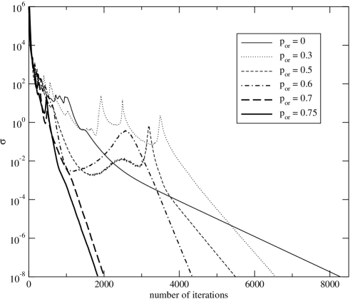
Figure A.1: Convergence of the Los Alamos gauge fixing algorithm for different values of the stochastic overrelaxation parameter $p_{\rm or}$ on a $9^{3}\times 24$ gauge configuration with $\beta=3.0$ fixed to Landau gauge. For $p_{\rm or}=0.8$ the algorithm did not converge, but stayed at $\sigma\approx 10^{-2}$ after $\sim 1000$ iterations.

A.2.2 Tuning of the Overrelaxation Parameter $p_{\rm or}$

It is easily possible to gain a factor of 4 in the number of iterations needed to reach a given gauge fixing accuracy when accelerating the algorithm by stochastic overrelaxation, as the gauge fixing procedure is very sensitive to the value of $p_{\rm or}$. Fig. A.1 shows a plot of the convergence history on one configuration in dependence of the stochastic parameter. The number of iterations needed to fix the gauge is reduced from over 8000 to below 2000 when setting $p_{\rm or}=0.75$. Unfortunately, the optimization of $p_{\rm or}$ is not a very stable procedure, and it can happen that for $p_{\rm or}>0$, the gauge fixing takes much longer on certain gauge configurations than on the others. As seen in Fig. A.2, this is related to the fact that shortly after the beginning, $\sigma$ starts to fluctuate wildly for some time, and only then a monotonic decrease is observed. A possible explanation of this behavior is that for a certain time it is not clear which Gribov copy the algorithm is going to choose. In Fig. A.3 we plot the difference of the gauge fixing functional (A.7) from its final value together with $\sigma$. Several plateaus in the value of $F_{U}$ show up before the algorithm decides which local minimum to take.

As soon as the region of monotonic decrease of $\sigma$ is reached, the convergence is much faster with stochastic overrelaxation than without. It is also obvious from Fig A.2 that small changes in $p_{\rm or}$ can lead to a very different behavior in this fluctuating region, resulting in factors of 2 in the total number of iterations. Still, compared to the $p_{\rm or}=0$ case, a significant reduction is achieved.

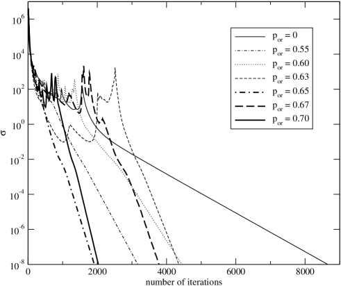
Figure A.2: Convergence of the Landau gauge fixing for different values of the stochastic overrelaxation parameter $p_{\rm or}$ on a $12^{3}\times 24$ gauge configuration with $\beta=3.4$. For $0.55\leq p_{\rm or}\leq 0.7$, the total number of iterations does not depend smoothly on the stochastic overrelaxation parameter. For $p_{\rm or}\geq 0.75$, the gauge fixing did not converge.

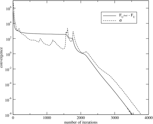
Figure A.3: The difference of the gauge fixing functional from its final value and the convergence criterion $\sigma$ for a $12^{3}\times 24$ gauge configuration with $\beta=3.4$ fixed to Landau gauge for $p_{\rm or}=0.67$. The plot shows that the algorithm tends to fall into several other local minima before finally converging.

In our tests, it appeared that a value of $p_{\rm or}$ slightly below the point where convergence is lost worked well in most cases. As the computer time needed for the gauge fixing was considerably smaller than for the generation of the gauge configurations, a further optimization of the procedure was not necessary.

A.3 Coulomb vs. Landau Gauge

When one decides to work in a fixed gauge background in order to measure the hadron spectrum with extended operators, one has to choose a specific gauge. There is a theoretical argument why Landau gauge is not well-suited for the measurement of time-dependent correlation functions $C(t)=\langle\mathcal{O}_{f}(t)\mathcal{O}_{i}(0)\rangle$ which are used to extract masses: Consider a gauge configuration $U$, which is fixed to Landau gauge:

$$U\longrightarrow U_{\rm gf}.$$ (A.13)

Suppose we measure a spatially extended, gauge-dependent operator $\mathcal{O}(U_{\rm gf},t=0)$ on the time slice $t=0$ of the gauge-fixed configuration. Such an operator might for example be the smeared source of a hadron correlator. Now change one single gauge link of the configuration $U$ on a time slice $t\neq 0$, for example by rotating it into the opposite direction:

$$U^{\prime}_{\mu}(x)=\left\{\begin{array}[]{ll}-U_{\mu}(x)&\mbox{if $\mu=1$ and $x=(x_{0},t_{0}\neq 0)$ },\\ \ \ U_{\mu}(x)&\mbox{otherwise}.\end{array}\right.$$ (A.14)

Fixing the resulting gauge configuration $U^{\prime}$ to Landau gauge,

$$U^{\prime}\longrightarrow U^{\prime}_{\rm gf},$$ (A.15)

the gauge-fixed configuration $U^{\prime}_{\rm gf}$ differs globally from $U_{\rm gf}$, since in the Landau gauge fixing process, spatial and temporal links enter in the minimizing functional (A.5). It follows that although the operator $\mathcal{O}$ is thought to be defined only on the time slice $t=0$, its value depends on the gauge fields on $t\neq 0$ time slices, and it is different on the two gauge fixed configurations:

$$\mathcal{O}(U_{\rm gf}^{\prime},t=0)\neq\mathcal{O}(U_{\rm gf},t=0).$$ (A.16)

Landau gauge fixing therefore introduces a non-local interaction in the time direction which might spoil the signal of hadron correlators.

The situation is different with Coulomb gauge: In the minimizing functional the links in the time direction do not enter, hence the gauge fixing is performed independently on each time slice. If a link on a time slice $t\neq 0$ is changed, the gauge fixed configuration on time slice $t=0$ is not affected, and the measured operator will not change.

In a study where hadron correlators with wall sources were compared on configurations fixed to both Coulomb and Landau gauge, a significant difference of order $3\sigma$ has been found for the mass of the $\Delta$ meson [167], which might be an effect of this non-local interaction in the Landau gauge fixing. For our hadron spectroscopy study, we therefore fix the configurations to Coulomb gauge.

Appendix B QCD on Large Computers

The non-perturbative approach to Quantum Chromodynamics as defined by the lattice regularization yields a theoretical formulation of the strong nuclear force which is ideal for treatment on large computers. The simulation of a realistic problem, like the scattering of two pions or the decay $K\rightarrow\pi\pi$, turns out to be a priori numerically very demanding due to the large number of degrees of freedom involved. The following arguments make it clear why lattice QCD calculations are hard: First, the spatial lattice volume has to be large enough, so that the wave functions of all involved particles fit into the box of side length $L_{s}=N_{s}a$ without getting squeezed. The temporal size $L_{t}=N_{t}a$ also has to be large, as one is mainly interested in the asymptotic behavior of correlation functions at large Euclidean time (see Chapter 5). Second, to get rid of discretization errors, the continuum limit $a\rightarrow 0$ has to be taken by performing simulations at several lattice spacings $a$ and extrapolating the measured observables to the continuum. This implies that it is necessary to work with lattice spacings $a$ small enough to ensure a controlled extrapolation, and therefore $N_{s}$ and $N_{t}$ get large quickly. Third, as the computational effort grows with inverse powers of the quark mass, simulations are mostly performed at values larger than the physical mass. Hence, another extrapolation from results calculated at several higher quark masses is necessary to obtain physical values.

As shown in Section 5.1.1, the numerically demanding part in quenched lattice QCD calculations is the inversion of the Dirac operator, which is a large sparse complex matrix of rank $4N_{c}V$ on a lattice with volume $V=N_{s}^{3}\times N_{t}$. This matrix inversion can be done very efficiently on massively parallel computers, because it boils down to many complex multiplication and addition operations, and only minimal communication is necessary between different processors. Large LQCD calculations are done either on commercial machines or on custom-built computers dedicated to lattice QCD. Commercial supercomputers are multi-purpose machines and have to perform well on a very diverse range of problems. Their architecture is therefore highly sophisticated in order to process all kinds of complex code efficiently. Due to the simple computational structure of lattice QCD calculations, building a dedicated computer is in general the much more cost-effective alternative. The lattice groups which have been running the largest simulations in the last few years all use custom-built machines: The Japanese CP-PACS computer in Tsukuba [168], several machines of the European APE project [169] and the Anglo-American QCDSP [170] computers and its successor QCDOC [171]. For our work, we had in contrary access to various multi-purpose machines spanning a large range from workstations to supercomputers. Tables B.1 and B.2 show the different platforms that were used for our simulations and their most relevant properties. The runs on the Hitachi were performed in the framework of the BGR collaboration [129].

Computer	Location	Type	$N_{\rm node}$	$N_{\rm CPU}$	$\nu_{\rm CPU}$
					[MHz]
AMD Athlon	ITP Bern	scalar	1	1	1200
AlphaServer DS20	ITP Bern	scalar	2	2	500
NEC SX-5/16	CSCS Manno	vector	10	10	250
IBM Power4	CSCS Manno	scalar	8	256	1300
Hitachi SR8000-F1	LRZ München	scalar	168	1344	375

Table B.1: Computers used for the simulations, with the number of nodes $N_{\rm node}$, the number of processors $N_{\rm CPU}$ and the CPU frequency $\nu_{\rm CPU}$. A node is defined here as the largest unit for which explicitly parallel code is not necessary. This might either be a single processor or a set of processors on which automatic parallelization by the compiler is provided.

Computer	$M_{\rm tot}$	$M_{\rm node}$	$P_{\rm tot}$	$P_{\rm node}$
	[GB]	[GB]	[GFLOPS]	[GFLOPS]
AMD Athlon	1	1	2	2
AlphaServer DS20	4	4	2	1
NEC SX-5/16	64	64	80	8
IBM Power4	768	96	1330	166
Hitachi SR8000-F1	928	8	2016	8

Table B.2: Main memory and performance of the different computers, each listed for the total machine and per node. The theoretical peak performance $P$ is given in units of $10^{9}$ floating point operations per second (GFLOPS).

In Appendix B.1, we summarize some technical details of the two computers we mostly worked on. Then we present in Appendix B.2 benchmark measurements from the spectroscopy simulations on the Hitachi and in particular the performance of our code under MPI parallelization. Finally we give in Appendix B.3 a brief introduction to modern matrix inversion algorithms and their extension to shifted linear systems, which is very useful for performing QCD simulations at many quark masses.

B.1 Specifications of Utilized Supercomputers

It is well-known that what is called a supercomputer at a given time might become inferior to a desktop PC only a few years later, and therefore technical details outdate quickly and are of marginal interest. But as for our simulations the architecture of the involved computers differed quite a lot, and the process of making the simulations run efficiently on the available platforms depends strongly on the technical details of the machines, we present the main properties of the two mostly used computers in some more detail.

B.1.1 The NEC SX-5/16

The Swiss Center for Scientific Computing in Manno installed in early 2000 a NEC SX-5 parallel-vector computer with eight processors and 64 GB of shared main memory. In 2001, two more processors were added. At the time it went operational, it was ranked at position 242 in the list of the top 500 supercomputers [172]. This computer differs from the other machines considered here by its vector architecture, which allows to obtain a very high single-processor performance: The basic building block is a 250 MHz CPU with 16 vector pipelines capable of processing two floating-point instructions each per clock cycle, leading to a theoretical peak performance of 8 GFLOPS per CPU. Although it is possible to run parallel processes, we only worked with scalar code due to the small number of installed processors and the long waiting time of the parallel queues.

The SX-5 is a good choice if one needs a lot of memory and does not want to write parallel code, as long as the problem is well-suited for vectorization. The compiler supports automatic vectorization, so it is possible to easily migrate existing scalar code from a workstation to the SX-5. However, to reach good performance, it is essential to optimize the time-critical parts by hand or with compiler directives. Moreover, code which does not vectorize well, like the algorithms used for the Monte Carlo update of the gauge configurations, ends up running extremely slow. The reason is that vector instructions need some time to be initialized, therefore the vectors have to be as long as possible in order to make the overhead irrelevant. In the program code, this manifests itself in the length of loops in which vector instructions appear. If these loops are not long enough, as it happens when doing manipulations on $SU(3)$ matrices, it is then even faster to run the program in scalar mode, which means that the machine is in this case inferior to every desktop computer due to its comparably low clock frequency.

B.1.2 The Hitachi SR8000-F1

A very different kind of architecture is provided by the Hitachi SR8000-F1 at Leibniz Rechenzentrum in München. This massively parallel scalar computer was also installed in early 2000 and was at that time the world’s fastest computer dedicated to academic research, ranked at 5th position of all supercomputers [172]. At installation time, it comprised of $112\times 8$ modified Power3 processors running at a clock frequency of 375 MHz. Each unit is able to process two multiply/add instructions simultaneously. Eight processors are grouped in a node, which can be treated by the programmer like a single CPU, and each node has access to 8 GB of main memory. The theoretical peak performance per node is $8\times 1.5=12$ GFLOPS. In January 2002, the machine was upgraded from 112 to 168 nodes, reaching more than 2 TFLOPS peak performance. The inter-node communication is realized with a multi-dimensional crossbar delivering a bi-directional peak bandwidth of 1 GB/s.

Programs running on the SR8000 have to be parallelized in order make use of multiple nodes. The parallelization within the eight processors of one node is automatically done by the compiler, which also provides a hardware-based ’pseudo-vectorization’ facility that imitates a vector processor. In our applications, it seemed that compared to a real vector computer, the SR8000 was more tolerant when running code that does not vectorize well, resulting in significantly better performance for such programs. However, to make full use of the computer’s capabilities, it is also necessary to tune the programs by optimizing the arrangement of array elements and loops and by placing appropriate compiler directives for parallelization and pseudo-vectorization at the time-critical code segments.

B.2 Measurements of Parallel Performance

For larger simulations on the Hitachi SR8000, explicitly parallel code is required. The common standard for programming the communication between different nodes of a computer or even different computers is the Message Passing Interface (MPI). In lattice QCD, explicit parallelization of the quark propagator code for $n$ nodes is in general a very simple task, since with an iterative solver the inversion of the Dirac operator reduces to matrix-vector multiplications. The Dirac operator can be split into $n$ parts containing $12V/n$ rows, and it only remains to write a distributed matrix-vector multiplication. However, for our implementation of the FP Dirac operator, parallelization is not completely trivial, because in the process of constructing the matrix it can occur that a gauge path calculated on a certain node needs to be stored on a different node. This is merely a consequence of the way our low-level routines for building the gauge paths in the Dirac operator are designed, and not a problem of the FP Dirac operator itself. Therefore, to make the construction of the Dirac operator work in parallel, some inter-node communication is needed. The Fixed-Point R operator is free of this complication, so parallelizing its construction is trivial. In order to have a completely parallel code, also the vectors of size $12V$ appearing in the different algorithms like the matrix inverter or the eigenvalue solver have to be distributed.

Not only in terms of computation time, but also in terms of storage the parallelization of the FP Dirac operator is crucial. The memory needed for storing the Dirac operator on a lattice of volume $V$ is $12\times 81\times 12\times V\times 16$ bytes, which exceeds the shared main memory available on most machines even at moderate lattice sizes. Table B.3 lists the storage requirements for various elements of our code at the lattice volumes used in the simulations.

array	$8^{3}\times 24$	$12^{3}\times 24$	$16^{3}\times 24$
$D^{\rm FP}$	2.1 GB	7.2 GB	22.8 GB
$R^{\rm FP}$	0.15 GB	0.5 GB	1.5 GB
$U$	6.8 MB	23 MB	72 MB
$b$	2.3 MB	7.6 MB	24 MB

Table B.3: Memory requirements for storing the parametrized FP Dirac and R operators, a gauge configuration $U$ and a vector $b$ of size $12V$ at different lattice volumes $V$.

	$8^{3}\times 24$		$12^{3}\times 24$		$16^{3}\times 24$
# nodes	$t_{\rm dot}$ [$ms$]	$\omega$	$t_{\rm dot}$ [$ms$]	$\omega$	$t_{\rm dot}$ [$ms$]	$\omega$
1	0.33	1.0	0.89	1.0	2.60	1.00
2	0.31	1.9	0.59	1.3	1.43	1.10
4	0.27	3.3	0.41	1.8	0.82	1.26
8	0.25	6.1	0.34	3.1	0.54	1.66
16	0.39	19	0.44	7.9	0.44	2.71

Table B.4: Time im milliseconds and overhead factor for dot product of two complex vectors of size $12V$ at different levels of MPI parallelization on the Hitachi SR8000. On the smallest volume, there is essentially no gain from parallelization.

	$8^{3}\times 24$		$12^{3}\times 24$		$16^{3}\times 32$
# nodes	$t_{D}$ [$s$]	$\omega$	$t_{D}$ [$s$]	$\omega$	$t_{D}$	$\omega$
1	347	1.00
2	192	1.11	610	1.00
4	98	1.13	323	1.06
8	57	1.31	188	1.16	930	1.00
16					570	1.23

Table B.5: Construction time in seconds and overhead factor for building up the Fixed-Point Dirac operator as a function of lattice size and parallelization level. There is a small parallelization overhead due to communication occurring when gauge paths cross node boundaries.

	$8^{3}\times 24$		$12^{3}\times 24$		$16^{3}\times 32$
# nodes	$t_{R}$ [$s$]	$\omega$	$t_{R}$ [$s$]	$\omega$	$t_{R}$	$\omega$
1	221	1.0
2	111	1.0	371	1.0
4	54	1.0	187	1.0
8	28	1.0	94	1.0	296	1.0
16					148	1.0

Table B.6: Construction time in seconds and overhead factor for building up the Fixed-Point R operator as a function of lattice size and parallelization level. No overhead for parallelization is seen, as there is no communication over node boundaries necessary.

	$8^{3}\times 24$		$12^{3}\times 24$		$12^{3}\times 24$		$16^{3}\times 32$
# nodes	(FP)		(FP)		(overlap)		(FP)
	$t_{\rm iter}$ [$s$]	$\omega$	$t_{\rm iter}$ [$s$]	$\omega$	$t_{\rm iter}$	$\omega$	$t_{\rm iter}$	$\omega$
1	0.564	1.00
2	0.313	1.11	1.045	1.00
4	0.185	1.31	0.619	1.18	5.36	1.00
8	0.122	1.73	0.405	1.55	3.57	1.33	1.30	1.00
16							1.05	1.62

Table B.7: Time im seconds and overhead factor for one iteration of the matrix inversion algorithm as a function of lattice size and parallelization level for the parametrized FP and the overlap Dirac operator. One iteration requires two matrix-vector products of both the Dirac and R operator and some additional dot products of two vectors. For the overlap, a third order Legendre expansion of the inverse square root is used with the 100 lowest eigenmodes treated exactly.

	$8^{3}\times 24$			$12^{3}\times 24$
# nodes	(FP)			(FP)
	$t_{D}$ [%]	$t_{R}$ [%]	MFLOPS	$t_{D}$ [%]	$t_{R}$ [%]	MFLOPS
1	56	16	4200
2	55	18	3800	60	19	4160
4	53	22	3240	59	23	3570
8	51	27	2560	57	29	2850

	$12^{3}\times 24$			$16^{3}\times 32$
# nodes	(overlap)			(FP)
	$t_{D}$ [%]	$t_{R}$ [%]	MFLOPS	$t_{D}$ [%]	$t_{R}$ [%]	MFLOPS
4	54	22	3660
8	50	26	2750	56	29	2770
16				51	34	1700

Table B.8: Overall performance measurements for typical quark propagator runs on the Hitachi SR8000. Shown are the percentage of the overall time spent for the $D$ and $R$ multiplication routines including communication of the input vector and the overall speed in MFLOPS per node with theoretical peak speed of 12 GFLOPS. The overall run time is measured from program start to finish and thus includes I/O time, MPI initialization and finalization and constructing of $D$ and $R$ operators.

It is clear that the communication between different nodes introduces an overhead, and that this parallelization overhead increases with the number of nodes. Therefore it is important to find a reasonable balance between the gain in wall-clock time and the loss in CPU time due to parallelization. To quantify the parallelization overhead, we list in Tables B.4–B.7 for several computational tasks the wall-clock time and the overhead factor $\omega$, which is defined as

$$\omega=n\frac{t_{n}}{t_{\rm ref}},$$ (B.1)

where $n$ is the number of nodes, $t_{n}$ is the wall clock time for the task running on $n$ nodes and $t_{\rm ref}$ is the wall-clock time for the smallest $n$ on which it was possible to run the task due to memory limitations. As shown in Table B.4, the dot product of two vectors does not really profit from parallelization on the smallest lattice. The situation changes drastically on the larger lattices, where the distribution of the vectors is crucial if one does not want to have severe slowing down in algorithms which perform many vector operations. For the construction of the FP Dirac operator (Table B.5), parallelization works well. The overhead introduced by the above mentioned inter-node communication is small for reasonable ratios of the lattice volume $V$ and the number of nodes $n$. That the construction of the $R$ operator parallelizes trivially can be seen in Table B.6.

The crucial quantity for quenched QCD simulations is the time needed for one iteration of the matrix inversion algorithm, which is listed in Table B.7. This is by far the most time-consuming task, and as one sees the overhead is still considerable. On the $12^{3}\times 24$ lattice, for example, there is only $50\%$ gain in time when going from 4 to 8 nodes, so it is advisable to run the simulations on the smallest $n$ possible for a given $V$. Comparing the results on the different lattice sizes running on 8 nodes shows that the time increases proportionally to the volume. Hence it seems that the code does not profit anymore from longer loops as they appear for larger volumes.

Typical benchmark measurements of the overall performance for the quark propagator inversion in hadron spectroscopy are given in Table B.8. These values depend on the number of iterations needed for the inversion of the Dirac operator, thus they only give an estimate for the performance of simulations in which the smallest quark mass is given by those used in our runs. The bottom line is that our code is reasonably efficient, running at an overall rate of around 30% of peak performance in the production runs. This number noticeably increases when considering only the matrix inversions, since the construction of the $D$ and $R$ operators and the time for I/O and MPI setup decrease overall performance: The matrix-vector multiplications without communication run at 6.3 GFLOPS per node for the Dirac operator $D$ and at 8.6 GFLOPS per node for the $R$ operator, which is remarkably fast.

B.3 Matrix Inversion Techniques

The key element for efficient simulations of quenched QCD is a fast matrix inversion algorithm. As the rank of the Dirac operator matrix is far too large to perform an exact inversion, the methods of choice are iterative procedures, and the most widely used algorithms for QCD are variants of Krylov subspace methods. Consider the linear system of equations

$$Mx=b,$$ (B.2)

where $M\in{\bf C}^{R\times R}$ is in general a non-hermitean matrix and $b\in{\bf C}^{R}$ is the source vector on which the inversion is carried out. Choosing an initial guess $x_{0}$, the initial residual $r_{0}=b-Mx_{0}$ is defined. The Krylov subspace $K^{n}$ is then given by

$$K^{n}={\rm span}\{M^{m}r_{0};m=0,\dots,n\}.$$ (B.3)

The common feature of all variants of Krylov space solvers is that the solution of (B.2) is iteratively approximated using an orthogonal basis of the Krylov subspace $K^{n}$. The iterative solution $x_{n}$ is of the form

$$x_{n}=x_{0}+q_{n-1}(M)r_{0},$$ (B.4)

where $q_{n-1}$ is a polynomial of maximum degree $n-1$. The iterative residual $r_{n}$ is therefore

$$r_{n}=\big{(}1-Mq_{n-1}(M)\big{)}r_{0}.$$ (B.5)

The best-known Krylov space solver is the Conjugate Gradient (CG) algorithm, which however only works for hermitean matrices. Refined types of algorithms are the Conjugate Gradient Squared (CGS) [173], Quasi-Minimal Residual (QMR) [174], Generalized Minimal Residual (GMRES) [175] or Bi-Conjugate Gradient (BiCG) [176] algorithms. These more sophisticated methods show either faster convergence or increased stability and are also applicable to non-hermitean matrices. We compared the convergence of the matrix inversion for several algorithms on a toy lattice of size $4^{4}$, with $M$ given by the parametrized FP Dirac operator. The results in Fig. B.1 show that the stabilized Bi-Conjugate Gradient (BiCGStab), transpose-free QMR and CGS algorithm perform comparably well in this test. The order $l$ in the BiCGStab($l$) variants denotes the order of the subspaces which are intermediately orthogonalized in the iteration process. Closer investigations of the properties of the different methods have shown that BiCGStab is in general a good and reliable choice [177, 178, 179].

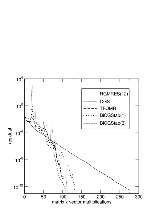
Figure B.1: Convergence history of quark propagator inversion for various algorithms. All but the RGMRES algorithm converge after a comparable number of matrix-vector multiplications. While CGS shows large fluctuations of the residual, the convergence of the transpose-free QMR (TFQMR) and BiCGStab is smoother.

As QCD simulations are in generally done at several quark masses, a significant computational gain can be obtained using multi-mass solvers [180], which exploit the fact that it is possible to get the solution of the shifted linear system

$$(M+\sigma)x=b,$$ (B.6)

for a whole set of values $\sigma\in{\bf C}$ at the cost of only one inversion. In QCD this implies that the cost of a multi-mass inversion is equivalent to the cost of a single inversion at the smallest quark mass. For our spectroscopy calculations, we worked with the multi-mass BiCGStab algorithm in [132]. The drawback of this method is that it is no longer possible to improve the condition number of $M$ by using preconditioning techniques, because the starting guess $x_{0}$ for the multi-mass inversion is required to be zero [132]. If one however wants to invert at a large number of quark masses, this disadvantage is more than compensated by the gain from needing only one inversion.

Appendix C Conditions on the Dirac Operator from Discrete Symmetries

While a lattice transcription of the continuum quark action allows many possible discretizations of the Dirac operator, it is essential that any lattice Dirac operator has the same properties under discrete symmetry transformations as in the continuum. We derive here the transformation properties under reflection of a coordinate axis and charge conjugation from the basic properties of the Dirac spinors and the gauge fields. The representation of the Clifford algebra which is used is given in Appendix E.

C.1 Reflection of an Axis

A reflection in direction of a coordinate axis $\eta$ with $\eta=1,\dots,4$ can be described by a unitary operator $\mathcal{P}_{\eta}=\mathcal{P}_{\eta}^{\Psi}\mathcal{P}_{\eta}^{U}$. The operator $\mathcal{P}_{\eta}^{\Psi}$ acts on the fermion fields,

$$\mathcal{P}_{\eta}^{\Psi}\Psi(n){\mathcal{P}_{\eta}^{\Psi}}^{-1} =P_{\eta}\Psi(\tilde{n}),$$ (C.1)

$$\mathcal{P}_{\eta}^{\Psi}\bar{\Psi}(n){\mathcal{P}_{\eta}^{\Psi}}^{-1} =\bar{\Psi}(\tilde{n})P_{\eta}^{-1},$$ (C.2)

where $\tilde{n}$ is the reflected lattice space-time variable,

$$\tilde{n}_{\mu}\equiv\begin{cases}-n_{\mu}\quad&\textrm{for }\mu=\eta,\\ n_{\mu}&\textrm{for }\mu\neq\eta,\end{cases}$$ (C.3)

and $P_{\eta}$ is a matrix in Dirac space (in our representation $P_{\eta}=\gamma_{\eta}\gamma_{5}$). On the other hand, $\mathcal{P}_{\eta}^{U}$ acts on the gauge fields,

$$\mathcal{P}_{\eta}^{U}U_{\mu}(n){\mathcal{P}_{\eta}^{U}}^{-1}=U_{\mu}^{\mathcal{P}_{\eta}}(n),$$ (C.4)

where the reflected gauge field $U_{\mu}^{\mathcal{P}_{\eta}}$ is defined as

$$U_{\mu}^{\mathcal{P}_{\eta}}(n)\equiv\begin{cases}U_{\eta}^{\dagger}(\tilde{n}-\hat{\eta})&\textrm{for }\mu=\eta,\\ U_{\mu}(\tilde{n})\quad&\textrm{for }\mu\neq\eta.\end{cases}$$ (C.5)

The lattice fermion action

$$S[\Psi,\bar{\Psi},U_{\mu}]=\sum_{n,n^{\prime}}\bar{\Psi}(n)D(n,n^{\prime},U_{\mu}(n))\Psi(n),$$ (C.6)

has to be symmetric under reflections of the $\eta$-axis:

$$S[\Psi,\bar{\Psi},U_{\mu}]=\mathcal{P}_{\eta}S[\Psi,\bar{\Psi},U_{\mu}]\mathcal{P}_{\eta}^{-1}.$$ (C.7)

Inserting the action (C.6) into (C.7) and using $\mathcal{P}_{\eta}\mathcal{P}_{\eta}^{-1}={\bf 1}$ twice, we get

$$S[\Psi,\bar{\Psi},U_{\mu}]=\sum_{n,n^{\prime}}\mathcal{P}_{\eta}\bar{\Psi}(n)\mathcal{P}_{\eta}^{-1}\mathcal{P}_{\eta}D(n,n^{\prime},U_{\mu}(n))\mathcal{P}_{\eta}^{-1}\mathcal{P}_{\eta}\Psi(n)\mathcal{P}_{\eta}^{-1}.$$ (C.8)

The fermion and gauge fields transform as specified in Eqs. (C.1)–(C.4):

$$S[\Psi,\bar{\Psi},U_{\mu}]=\sum_{n,n^{\prime}}\bar{\Psi}(\tilde{n})P_{\eta}^{-1}D(n,n^{\prime},U_{\mu}^{\mathcal{P}_{\eta}}(n))P_{\eta}\Psi(\tilde{n}).$$ (C.9)

It remains to reorder the summation over the $\eta$-component of the lattice variables $n$ and $n^{\prime}$. As it does not matter whether the sum over a variable is performed from above or from below,

$$\sum_{n_{\eta}=-\infty}^{\infty}F(n)=\sum_{n_{\eta}=\infty}^{-\infty}F(n)=\sum_{n_{\eta}=-\infty}^{\infty}F(\tilde{n}),$$ (C.10)

the argument of the summand can be reflected without changing the value of the sum. Applying this to Eq. (C.9), we get

$$S[\Psi,\bar{\Psi},U_{\mu}]=\sum_{n,n^{\prime}}\bar{\Psi}(n)P_{\eta}^{-1}D(\tilde{n},\tilde{n}^{\prime},U_{\mu}^{\mathcal{P}_{\eta}}(\tilde{n}))P_{\eta}\Psi(n),$$ (C.11)

which provides us the condition for the Dirac operator

$$D(n,n^{\prime},U_{\mu}(n))=P_{\eta}^{-1}D(\tilde{n},\tilde{n}^{\prime},U_{\mu}^{\mathcal{P}_{\eta}}(\tilde{n}))P_{\eta}\,,$$ (C.12)

when comparing with the original action (C.6).

C.2 Charge Conjugation

The unitary charge conjugation operator $\mathcal{C}$ acts on the fermion and gauge fields like [181]

$$\mathcal{C}\Psi\mathcal{C}^{-1} =C\bar{\Psi}^{T},$$ (C.13)

$$\mathcal{C}\bar{\Psi}\mathcal{C}^{-1} =\Psi^{T}C^{-1},$$ (C.14)

$$\mathcal{C}U_{\mu}\mathcal{C}^{-1} =U_{\mu}^{*},$$ (C.15)

where the charge conjugation matrix fulfills $C\gamma_{\mu}^{T}C^{-1}=-\gamma_{\mu}$ and can be expressed in our representation by $C=\gamma_{2}\gamma_{4}$. Invariance of the action under $\mathcal{C}$-transformations means

$$\bar{\Psi}D(U_{\mu})\Psi=\mathcal{C}\bar{\Psi}D(U_{\mu})\Psi\mathcal{C}^{-1}.$$ (C.16)

Inserting $\mathcal{C}^{-1}\mathcal{C}$ twice and using $C^{T}=C^{-1}$, we get

$$\bar{\Psi}D(U_{\mu})\Psi =\Psi^{T}C^{-1}D(U_{\mu}^{*})C\bar{\Psi}^{T}$$

$$=\bar{\Psi}C^{-1}D(U_{\mu}^{*})^{T}C\Psi,$$ (C.17)

where the transposition extends over all index spaces. The transformation property of the Dirac operator under charge conjugation is therefore

$$D(U_{\mu})=C^{-1}D(U_{\mu}^{*})^{T}C,$$ (C.18)

completing the set of conditions from the $\mathcal{C}$, $\mathcal{P}$ and (Euclidean) $\mathcal{T}$ symmetries.

Appendix D Collection of Data

D.1 Hadron Masses

For each lattice, we list the bare input quark masses, the bias-corrected masses from correlated fits to the hadron propagators, the value of $\chi^{2}/df$ for the fit and the fit range. The numbers in brackets and the superscripts denote bootstrap errors and bias (5.40), respectively.

D.1.1 Pseudoscalar Mesons

Pseudoscalar mesons are determined from the pseudoscalar (P), fourth component axial vector (A), and pseudoscalar minus scalar (P-S) correlators.

$8^{3}\times 24$, $\beta=3.0$, parametrized FP
$am_{q}$	$am_{\rm PS}$(P)	$\chi^{2}_{df}$	$t$	$am_{\rm PS}$(A)	$\chi^{2}_{df}$	$t$	$am_{\rm PS}$(P-S)	$\chi^{2}_{df}$	$t$
0.021	$0.240(15)^{+8}$	1.9	[4,12]	$0.254(13)^{-1}$	0.7	[5,12]	$0.198(16)^{+8}$	2.3	[4,12]
0.028	$0.289(9)^{+2}$	2.4	[4,12]	$0.288(9)^{+0}$	0.9	[5,12]	$0.246(13)^{+6}$	2.3	[5,12]
0.04	$0.345(7)^{+2}$	2.6	[4,12]	$0.335(7)^{+1}$	1.4	[5,12]	$0.326(9)^{+2}$	3.0	[5,12]
0.06	$0.415(6)^{+2}$	2.4	[4,12]	$0.405(6)^{+1}$	1.8	[5,12]	$0.413(7)^{+1}$	3.2	[5,12]
0.09	$0.503(5)^{+1}$	2.2	[4,12]	$0.495(5)^{+1}$	1.9	[5,12]	$0.508(5)^{+1}$	3.6	[6,12]
0.13	$0.606(3)^{+1}$	2.0	[4,12]	$0.599(4)^{+1}$	1.8	[5,12]	$0.614(4)^{+1}$	3.3	[6,12]
0.18	$0.720(3)^{+1}$	1.7	[4,12]	$0.714(3)^{+1}$	1.7	[5,12]	$0.728(3)^{+0}$	2.8	[6,12]
0.25	$0.866(2)^{+0}$	1.6	[4,12]	$0.862(2)^{+1}$	1.8	[5,12]	$0.875(3)^{+0}$	2.2	[6,12]
0.33	$1.024(2)^{+0}$	1.8	[4,12]	$1.022(2)^{+0}$	2.1	[5,12]	$1.031(3)^{+0}$	1.9	[7,12]

Table D.1: Pseudoscalar meson masses on $8^{3}\times 24$ lattice at $\beta=3.0$ with $D^{\rm FP}$.

$12^{3}\times 24$, $\beta=3.0$, parametrized FP
$am_{q}$	$am_{\rm PS}$(P)	$\chi^{2}_{df}$	$t$	$am_{\rm PS}$(A)	$\chi^{2}_{df}$	$t$	$am_{\rm PS}$(P-S)	$\chi^{2}_{df}$	$t$
0.016	$0.2300(51)^{-8}$	0.9	[4,12]	$0.2177(50)^{-2}$	2.2	[4,12]	$0.2020(70)^{+22}$	0.6	[6,12]
0.021	$0.2555(33)^{-2}$	0.6	[4,12]	$0.2472(41)^{+4}$	1.5	[4,12]	$0.2409(51)^{+10}$	0.6	[6,12]
0.028	$0.2881(27)^{+1}$	0.6	[4,12]	$0.2840(35)^{+2}$	0.9	[4,12]	$0.2809(43)^{+9}$	0.5	[6,12]
0.04	$0.3382(20)^{+2}$	0.5	[4,12]	$0.3359(29)^{+2}$	0.5	[4,12]	$0.3362(37)^{+5}$	0.4	[6,12]
0.06	$0.4090(16)^{+2}$	0.4	[4,12]	$0.4077(25)^{+1}$	0.5	[4,12]	$0.4099(27)^{+2}$	0.6	[7,12]
0.09	$0.4987(14)^{+1}$	0.7	[4,12]	$0.4972(22)^{+0}$	1.1	[4,12]	$0.5009(22)^{+1}$	0.9	[7,12]
0.13	$0.6016(13)^{+1}$	1.3	[4,12]	$0.6001(17)^{+2}$	2.2	[4,12]	$0.6052(17)^{+0}$	0.8	[7,12]
0.18	$0.7165(11)^{+1}$	1.8	[4,12]	$0.7151(15)^{+1}$	3.3	[4,12]	$0.7213(15)^{+0}$	0.7	[7,12]
0.25	$0.8640(11)^{+0}$	2.1	[4,12]	$0.8624(13)^{+1}$	4.5	[4,12]	$0.8703(14)^{+0}$	0.7	[7,12]
0.33	$1.0229(11)^{+1}$	2.2	[4,12]	$1.0212(12)^{+1}$	5.5	[4,12]	$1.0304(13)^{+1}$	1.1	[7,12]

Table D.2: Pseudoscalar meson masses on $12^{3}\times 24$ lattice at $\beta=3.0$ with $D^{\rm FP}$.

$12^{3}\times 24$, $\beta=3.0$, overlap-improved
$am_{q}$	$am_{\rm PS}$(P)	$\chi^{2}_{df}$	$t$	$am_{\rm PS}$(A)	$\chi^{2}_{df}$	$t$	$am_{\rm PS}$(P-S)	$\chi^{2}_{df}$	$t$
0.009	$0.196(11)^{+3}$	2.1	[4,12]	$0.218(6)^{+0}$	1.3	[4,12]	$0.154(14)^{+7}$	1.4	[4,12]
0.012	$0.217(9)^{+2}$	2.0	[4,12]	$0.235(6)^{+0}$	1.1	[4,12]	$0.185(13)^{+6}$	1.2	[4,12]
0.016	$0.245(6)^{+2}$	2.0	[4,12]	$0.256(5)^{+1}$	1.0	[4,12]	$0.221(12)^{+5}$	1.3	[4,12]
0.021	$0.274(5)^{+2}$	1.9	[4,12]	$0.282(5)^{+1}$	1.2	[4,12]	$0.258(10)^{+4}$	1.7	[5,12]
0.028	$0.309(4)^{+1}$	1.9	[4,12]	$0.315(4)^{+1}$	1.6	[4,12]	$0.300(7)^{+3}$	2.0	[5,12]
0.04	$0.360(3)^{+1}$	1.8	[4,12]	$0.363(4)^{+0}$	1.9	[4,12]	$0.355(6)^{+2}$	2.2	[5,12]
0.06	$0.433(3)^{+1}$	1.9	[4,12]	$0.432(3)^{+1}$	2.3	[4,12]	$0.428(4)^{+1}$	2.3	[6,12]
0.09	$0.526(2)^{+1}$	2.3	[4,12]	$0.524(3)^{+1}$	2.6	[4,12]	$0.525(3)^{+1}$	2.0	[6,12]
0.13	$0.633(2)^{+1}$	2.5	[4,12]	$0.631(2)^{+1}$	2.9	[4,12]	$0.634(2)^{+1}$	2.3	[7,12]
0.18	$0.753(2)^{+1}$	2.5	[4,12]	$0.752(2)^{+0}$	3.1	[4,12]	$0.756(2)^{+0}$	1.9	[7,12]
0.25	$0.905(2)^{+0}$	2.1	[4,12]	$0.905(2)^{+0}$	3.1	[4,12]	$0.911(2)^{+0}$	1.7	[7,12]
0.33	$1.069(1)^{+0}$	1.7	[4,12]	$1.069(2)^{+0}$	3.2	[4,12]	$1.076(2)^{+0}$	1.7	[7,12]

Table D.3: Pseudoscalar meson masses on $12^{3}\times 24$ lattice at $\beta=3.0$ with the overlap-improved $D_{\rm ov}^{\rm FP}$.

$16^{3}\times 32$, $\beta=3.0$, parametrized FP
$am_{q}$	$am_{\rm PS}$(P)	$\chi^{2}_{df}$	$t$	$am_{\rm PS}$(A)	$\chi^{2}_{df}$	$t$	$am_{\rm PS}$(P-S)	$\chi^{2}_{df}$	$t$
0.013	$0.1984(31)^{+7}$	1.2	[4,16]	$0.1984(33)^{+6}$	0.8	[4,16]	$0.1904(28)^{+17}$	0.9	[4,16]
0.016	$0.2224(19)^{+3}$	1.2	[4,16]	$0.2227(26)^{+3}$	0.7	[4,16]	$0.2168(22)^{+10}$	0.9	[4,16]
0.021	$0.2534(16)^{+2}$	1.0	[4,16]	$0.2538(24)^{+3}$	0.5	[4,16]	$0.2500(18)^{+7}$	0.9	[4,16]
0.028	$0.2892(13)^{+2}$	0.8	[4,16]	$0.2893(20)^{+3}$	0.4	[4,16]	$0.2862(16)^{+5}$	0.7	[6,16]
0.04	$0.3402(13)^{+0}$	0.8	[5,16]	$0.3399(17)^{+2}$	0.3	[4,16]	$0.3389(15)^{+4}$	0.5	[6,16]
0.06	$0.4109(12)^{+1}$	0.7	[5,16]	$0.4100(14)^{+3}$	0.1	[4,16]	$0.4116(14)^{+2}$	0.4	[6,16]
0.09	$0.5000(10)^{+2}$	0.7	[5,16]	$0.4988(13)^{+2}$	0.1	[4,16]	$0.5017(15)^{+0}$	0.5	[8,16]
0.13	$0.6022(10)^{+1}$	0.6	[6,16]	$0.6012(11)^{+2}$	0.2	[4,16]	$0.6045(12)^{+1}$	1.0	[9,16]
0.18	$0.7173(9)^{+1}$	0.8	[6,16]	$0.7160(10)^{+1}$	0.3	[4,16]	$0.7196(11)^{+1}$	1.5	[9,16]
0.25	$0.8649(9)^{+1}$	0.8	[6,16]	$0.8639(9)^{+1}$	0.2	[5,16]	$0.8665(11)^{+0}$	1.7	[11,16]
0.33	$1.0239(8)^{+1}$	0.6	[6,16]	$1.0230(8)^{+1}$	0.2	[5,16]	$1.0256(11)^{+1}$	1.1	[11,16]

Table D.4: Pseudoscalar meson masses on $16^{3}\times 32$ lattice at $\beta=3.0$ with $D^{\rm FP}$.

$12^{3}\times 24$, $\beta=3.4$, parametrized FP
$am_{q}$	$am_{\rm PS}$(P)	$\chi^{2}_{df}$	$t$	$am_{\rm PS}$(A)	$\chi^{2}_{df}$	$t$	$am_{\rm PS}$(P-S)	$\chi^{2}_{df}$	$t$
0.029	$0.191(6)^{+0}$	1.3	[4,12]	$0.183(5)^{-1}$	0.3	[3,12]	$0.159(9)^{+3}$	0.5	[7,12]
0.032	$0.203(4)^{+0}$	1.1	[4,12]	$0.197(5)^{-1}$	0.4	[3,12]	$0.170(9)^{+3}$	0.3	[8,12]
0.037	$0.224(4)^{+0}$	1.1	[4,12]	$0.218(4)^{+0}$	0.6	[3,12]	$0.197(8)^{+2}$	0.2	[8,12]
0.045	$0.251(5)^{+0}$	2.3	[7,12]	$0.248(4)^{+0}$	0.9	[3,12]	$0.234(11)^{+1}$	0.0	[10,12]
0.058	$0.294(3)^{+0}$	2.8	[7,12]	$0.291(3)^{+0}$	1.4	[3,12]	$0.287(8)^{+0}$	0.0	[10,12]
0.078	$0.355(3)^{+0}$	3.3	[7,12]	$0.352(2)^{+0}$	1.8	[3,12]	$0.355(6)^{+0}$	0.4	[10,12]
0.1	$0.415(2)^{+0}$	3.9	[7,12]	$0.411(2)^{+0}$	1.8	[3,12]	$0.417(4)^{+0}$	1.4	[10,12]
0.14	$0.514(2)^{+0}$	4.3	[7,12]	$0.509(2)^{+0}$	1.5	[3,12]	$0.518(3)^{+0}$	4.0	[10,12]
0.18	$0.603(2)^{+0}$	4.3	[7,12]	$0.598(1)^{+0}$	1.2	[3,12]	$0.609(2)^{+0}$	6.8	[10,12]
0.24	$0.729(1)^{+0}$	3.8	[7,12]	$0.723(1)^{+0}$	1.0	[3,12]	$0.736(2)^{+0}$	9.1	[10,12]

Table D.5: Pseudoscalar meson masses on $12^{3}\times 24$ lattice at $\beta=3.4$ with $D^{\rm FP}$.

$16^{3}\times 32$, $\beta=3.7$, parametrized FP
$am_{q}$	$am_{\rm PS}$(P)	$\chi^{2}_{df}$	$t$	$am_{\rm PS}$(A)	$\chi^{2}_{df}$	$t$	$am_{\rm PS}$(P-S)	$\chi^{2}_{df}$	$t$
0.0235	$0.133(11)^{-4}$	0.6	[6,16]	$0.120(8)^{+2}$	0.7	[7,16]	$0.120(12)^{+5}$	2.2	[7,14]
0.026	$0.143(8)^{-2}$	0.8	[6,16]	$0.134(6)^{+2}$	0.8	[7,16]	$0.135(10)^{+3}$	2.0	[7,15]
0.03	$0.159(6)^{-1}$	1.0	[6,16]	$0.153(6)^{+1}$	0.7	[7,16]	$0.155(7)^{+2}$	2.0	[7,15]
0.036	$0.183(4)^{+0}$	1.2	[6,16]	$0.177(5)^{+1}$	0.4	[7,16]	$0.186(6)^{+2}$	2.1	[7,15]
0.045	$0.216(3)^{+1}$	1.4	[6,16]	$0.210(4)^{+2}$	0.4	[7,16]	$0.225(5)^{+2}$	2.2	[8,16]
0.06	$0.264(3)^{+1}$	1.4	[6,16]	$0.258(4)^{+1}$	0.8	[7,16]	$0.277(4)^{+1}$	1.5	[8,16]
0.08	$0.321(2)^{+0}$	1.1	[6,16]	$0.315(3)^{+1}$	0.9	[7,16]	$0.335(3)^{+0}$	1.1	[9,16]
0.1	$0.372(2)^{+1}$	0.9	[6,16]	$0.368(2)^{+1}$	1.0	[7,16]	$0.386(3)^{+0}$	1.1	[9,16]
0.14	$0.465(1)^{+0}$	0.9	[6,16]	$0.463(2)^{+0}$	0.6	[8,16]	$0.478(2)^{+0}$	1.6	[9,16]
0.18	$0.550(1)^{+0}$	1.4	[6,16]	$0.549(1)^{+0}$	0.8	[8,16]	$0.562(2)^{+0}$	1.7	[9,16]

Table D.6: Pseudoscalar meson masses on $16^{3}\times 32$ lattice at $\beta=3.7$ with $D^{\rm FP}$.

D.1.2 Vector Mesons, $m_{\rm PS}/m_{\rm V}$ and $m_{\rm Oct}/m_{\rm V}$

Together with the bias-corrected fitted masses for the vector meson, we list the mass ratios $m_{\rm PS}/m_{\rm V}$ and $m_{\rm Oct}/m_{\rm V}$, where the pseudoscalar mass is taken from fits to the P-S correlator at small and the P correlator at large quark mass.

$8^{3}\times 24$, $\beta=3.0$, parametrized FP
$am_{q}$	$am_{\rm V}$	$\chi^{2}_{df}$	$t$	$m_{\rm PS}/m_{\rm V}$	$m_{\rm Oct}/m_{\rm V}$
0.021	$0.722(21)^{+2}$	1.5	[4,12]	0.274(24)	N/A
0.028	$0.706(17)^{+6}$	1.3	[4,12]	0.349(21)	1.221(21)
0.04	$0.711(13)^{+5}$	1.2	[4,12]	0.485(13)	1.396(64)
0.06	$0.738(12)^{+4}$	1.2	[4,12]	0.562(12)	1.429(40)
0.09	$0.780(9)^{+2}$	1.4	[4,12]	0.645(10)	1.455(29)
0.13	$0.837(7)^{+3}$	1.6	[4,12]	0.724(7)	1.486(20)
0.18	$0.912(5)^{+2}$	1.4	[4,12]	0.789(6)	1.508(15)
0.25	$1.024(4)^{+2}$	1.1	[4,12]	0.846(4)	1.524(11)
0.33	$1.155(3)^{+1}$	1.1	[4,12]	0.887(3)	1.531(8)

$12^{3}\times 24$, $\beta=3.0$, parametrized FP
$am_{q}$	$am_{\rm V}$	$\chi^{2}_{df}$	$t$	$m_{\rm PS}/m_{\rm V}$	$m_{\rm Oct}/m_{\rm V}$
0.016	$0.676(14)^{+2}$	1.7	[4,12]	0.299(12)	1.230(97)
0.021	$0.683(12)^{+1}$	1.7	[4,12]	0.353(9)	1.247(51)
0.028	$0.691(9)^{+2}$	1.6	[4,12]	0.406(8)	1.260(38)
0.04	$0.708(7)^{+1}$	1.7	[4,12]	0.475(7)	1.285(25)
0.06	$0.736(5)^{+0}$	1.8	[4,12]	0.556(4)	1.337(18)
0.09	$0.779(3)^{+0}$	1.7	[4,12]	0.641(3)	1.395(12)
0.13	$0.838(3)^{+0}$	1.6	[4,12]	0.718(3)	1.443(8)
0.18	$0.914(2)^{+0}$	1.5	[4,12]	0.784(2)	1.480(6)
0.25	$1.026(2)^{+0}$	1.2	[4,12]	0.842(2)	1.510(5)
0.33	$1.156(1)^{+0}$	0.8	[4,12]	0.885(1)	1.526(4)

$16^{3}\times 32$, $\beta=3.0$, parametrized FP
$am_{q}$	$am_{\rm V}$	$\chi^{2}_{df}$	$t$	$m_{\rm PS}/m_{\rm V}$	$m_{\rm Oct}/m_{\rm V}$
0.013	$0.692(16)^{+2}$	1.7	[5,16]	0.275(7)	1.226(39)
0.016	$0.696(14)^{+0}$	1.9	[5,16]	0.312(7)	1.228(32)
0.021	$0.702(10)^{+0}$	2.0	[5,16]	0.356(5)	1.241(24)
0.028	$0.711(8)^{+0}$	2.0	[5,16]	0.403(5)	1.261(20)
0.04	$0.724(6)^{+0}$	1.8	[5,16]	0.468(4)	1.297(16)
0.06	$0.748(4)^{+0}$	1.3	[5,16]	0.549(3)	1.347(13)
0.09	$0.787(3)^{+0}$	1.2	[5,16]	0.635(3)	1.400(10)
0.13	$0.843(2)^{+0}$	1.5	[5,16]	0.714(2)	1.448(7)
0.18	$0.918(2)^{+0}$	1.6	[5,16]	0.781(2)	1.484(6)
0.25	$1.029(1)^{+0}$	1.4	[5,16]	0.841(1)	1.511(4)
0.33	$1.160(1)^{+0}$	1.1	[5,16]	0.883(1)	1.526(3)

Table D.7: Vector meson masses and mass ratios $m_{\rm PS}/m_{\rm V}$ and $m_{\rm Oct}/m_{\rm V}$ on the three lattice of size $8^{3}\times 24$, $12^{3}\times 24$ and $16^{3}\times 32$ at $\beta=3.0$ with $D^{\rm FP}$.

$12^{3}\times 24$, $\beta=3.0$, overlap-improved
$am_{q}$	$am_{\rm V}$	$\chi^{2}_{df}$	$t$	$m_{\rm PS}/m_{\rm V}$	$m_{\rm Oct}/m_{\rm V}$
0.009	$0.747(31)^{+6}$	2.7	[3,11]	0.206(21)	1.297(123)
0.012	$0.743(26)^{+5}$	2.4	[3,11]	0.249(19)	1.274(96)
0.016	$0.746(21)^{+6}$	1.9	[3,11]	0.297(18)	1.253(68)
0.021	$0.752(16)^{+5}$	1.5	[3,11]	0.343(15)	1.241(51)
0.028	$0.754(26)^{+7}$	1.6	[4,11]	0.398(17)	1.264(54)
0.04	$0.766(19)^{+4}$	1.4	[4,11]	0.463(14)	1.297(42)
0.06	$0.789(13)^{+2}$	1.1	[4,11]	0.543(10)	1.353(31)
0.09	$0.826(7)^{+1}$	0.9	[4,11]	0.635(7)	1.397(20)
0.13	$0.883(5)^{+1}$	0.9	[4,11]	0.717(5)	1.434(15)
0.18	$0.962(4)^{+1}$	1.0	[4,11]	0.783(4)	1.469(10)
0.25	$1.077(3)^{+0}$	0.8	[4,11]	0.841(3)	1.500(8)
0.33	$1.212(2)^{+0}$	0.5	[4,11]	0.882(2)	1.518(7)

Table D.8: Vector meson masses and mass ratios on the $12^{3}\times 24$ lattice at $\beta=3.0$ with overlap-improved $D_{\rm ov}^{\rm FP}$.

$12^{3}\times 24$, $\beta=3.4$, parametrized FP
$am_{q}$	$am_{\rm V}$	$\chi^{2}_{df}$	$t$	$m_{\rm PS}/m_{\rm V}$	$m_{\rm Oct}/m_{\rm V}$
0.029	$0.470(20)^{+2}$	0.5	[7,12]	0.339(25)	1.428(87)
0.032	$0.474(17)^{+1}$	0.6	[7,12]	0.359(24)	1.433(76)
0.037	$0.482(13)^{+1}$	0.7	[7,12]	0.410(21)	1.444(58)
0.045	$0.492(10)^{+1}$	0.7	[7,12]	0.475(25)	1.473(43)
0.058	$0.509(8)^{+1}$	0.7	[7,12]	0.563(19)	1.503(31)
0.078	$0.540(6)^{+1}$	1.1	[7,12]	0.651(9)	1.513(25)
0.1	$0.576(5)^{+1}$	1.6	[7,12]	0.713(7)	1.523(21)
0.14	$0.644(3)^{+0}$	2.1	[7,12]	0.791(5)	1.525(15)
0.18	$0.712(3)^{+0}$	2.2	[7,12]	0.840(4)	1.531(12)
0.24	$0.817(2)^{+0}$	1.8	[7,12]	0.886(3)	1.534(8)

Table D.9: Vector meson masses and mass ratios $m_{\rm PS}/m_{\rm V}$ and $m_{\rm Oct}/m_{\rm V}$ on $12^{3}\times 24$ lattice at $\beta=3.4$ with $D^{\rm FP}$.

$16^{3}\times 32$, $\beta=3.7$, parametrized FP
$am_{q}$	$am_{\rm V}$	$\chi^{2}_{df}$	$t$	$m_{\rm PS}/m_{\rm V}$	$m_{\rm Oct}/m_{\rm V}$
0.0235	$0.332(26)^{+11}$	1.4	[8,16]	0.360(37)	1.595(75)
0.026	$0.337(22)^{+9}$	1.0	[8,16]	0.397(33)	1.582(33)
0.03	$0.346(18)^{+7}$	0.9	[8,16]	0.441(30)	1.570(9)
0.036	$0.366(13)^{+5}$	1.1	[8,16]	0.485(22)	1.528(70)
0.045	$0.386(10)^{+3}$	1.3	[8,16]	0.544(19)	1.496(52)
0.06	$0.411(8)^{+2}$	1.4	[8,16]	0.629(15)	1.486(40)
0.08	$0.443(6)^{+2}$	1.2	[8,16]	0.712(12)	1.495(28)
0.1	$0.477(4)^{+1}$	1.1	[8,16]	0.770(9)	1.508(22)
0.14	$0.547(3)^{+1}$	1.1	[8,16]	0.846(6)	1.523(15)
0.18	$0.618(2)^{+1}$	1.3	[8,16]	0.888(4)	1.530(10)

Table D.10: Vector meson masses and mass ratios $m_{\rm PS}/m_{\rm V}$ and $m_{\rm Oct}/m_{\rm V}$ on $16^{3}\times 32$ lattice at $\beta=3.7$ with $D^{\rm FP}$.

D.1.3 Octet Baryons

For each lattice, the bias-corrected fitted masses for the N and N0 correlators, the value of $\chi^{2}/df$ for the fit and the fit range are given. The correlator which was used for the ratio $m_{\rm Oct}/m_{\rm V}$ is marked with a star in each table.

$8^{3}\times 24$, $\beta=3.0$, parametrized FP
$am_{q}$	$am_{\rm Oct}$(N)∗	$\chi^{2}_{df}$	$t$	$am_{\rm Oct}$(N0)	$\chi^{2}_{df}$	$t$
0.028	$0.862(82)^{+29}$	1.0	[4,12]	$1.024(54)^{+15}$	0.7	[4,12]
0.04	$0.993(41)^{+0}$	1.8	[4,12]	$1.043(39)^{+11}$	0.7	[4,12]
0.06	$1.055(23)^{+2}$	2.0	[4,12]	$1.090(28)^{+11}$	1.2	[4,12]
0.09	$1.135(18)^{+4}$	1.6	[4,12]	$1.165(20)^{+9}$	1.8	[4,12]
0.13	$1.243(12)^{+4}$	1.3	[4,12]	$1.258(14)^{+7}$	2.1	[4,12]
0.18	$1.376(10)^{+4}$	1.2	[4,12]	$1.383(10)^{+6}$	2.0	[4,12]
0.25	$1.560(9)^{+4}$	1.2	[4,12]	$1.563(8)^{+4}$	2.1	[4,12]
0.33	$1.768(7)^{+3}$	1.7	[4,12]	$1.771(7)^{+3}$	2.4	[4,12]

$12^{3}\times 24$, $\beta=3.0$, parametrized FP
$am_{q}$	$am_{\rm Oct}$(N)∗	$\chi^{2}_{df}$	$t$	$am_{\rm Oct}$(N0)	$\chi^{2}_{df}$	$t$
0.016	$0.832(63)^{+0}$	1.3	[4,12]	$0.755(34)^{+20}$	0.8	[3,12]
0.021	$0.852(32)^{+1}$	1.2	[4,12]	$0.829(23)^{+7}$	1.5	[3,12]
0.028	$0.871(23)^{+3}$	1.1	[4,12]	$0.868(17)^{+3}$	1.9	[3,12]
0.04	$0.910(15)^{+2}$	0.9	[4,12]	$0.918(13)^{+2}$	1.9	[3,12]
0.06	$0.983(11)^{+2}$	1.2	[4,12]	$0.991(9)^{+2}$	1.4	[3,12]
0.09	$1.086(8)^{+2}$	1.9	[4,12]	$1.089(7)^{+2}$	1.2	[3,12]
0.13	$1.208(6)^{+1}$	1.8	[4,12]	$1.210(5)^{+1}$	1.2	[3,12]
0.18	$1.353(4)^{+1}$	1.4	[4,12]	$1.355(5)^{+1}$	1.3	[3,12]
0.25	$1.549(4)^{+1}$	1.2	[4,12]	$1.548(4)^{+1}$	1.6	[3,12]
0.33	$1.765(4)^{+1}$	1.4	[4,12]	$1.763(4)^{+1}$	1.9	[3,12]

$16^{3}\times 32$, $\beta=3.0$, parametrized FP
$am_{q}$	$am_{\rm Oct}$(N)	$\chi^{2}_{df}$	$t$	$am_{\rm Oct}$(N0)∗	$\chi^{2}_{df}$	$t$
0.013	$0.766(31)^{+19}$	1.1	[4,16]	$0.848(18)^{+1}$	0.9	[3,16]
0.016	$0.799(19)^{+6}$	1.2	[4,16]	$0.855(13)^{+1}$	1.2	[3,16]
0.021	$0.833(12)^{+3}$	1.5	[4,16]	$0.871(11)^{+1}$	1.5	[3,16]
0.028	$0.872(10)^{+2}$	1.6	[4,16]	$0.896(9)^{+1}$	1.8	[3,16]
0.04	$0.927(8)^{+1}$	1.4	[4,16]	$0.939(8)^{+1}$	1.9	[3,16]
0.06	$1.004(6)^{+1}$	1.0	[4,16]	$1.007(7)^{+2}$	1.3	[3,16]
0.09	$1.101(5)^{+1}$	0.7	[4,16]	$1.102(6)^{+2}$	0.6	[3,16]
0.13	$1.221(4)^{+1}$	0.9	[4,16]	$1.220(5)^{+2}$	0.8	[3,16]
0.18	$1.364(4)^{+1}$	1.2	[4,16]	$1.362(4)^{+2}$	1.1	[3,16]
0.25	$1.558(3)^{+2}$	1.3	[4,16]	$1.555(4)^{+2}$	1.0	[3,16]
0.33	$1.773(3)^{+1}$	1.3	[4,16]	$1.770(3)^{+1}$	0.8	[3,16]

Table D.11: Octet baryon masses on three lattice of size $8^{3}\times 24$, $12^{3}\times 24$ and $16^{3}\times 32$ at $\beta=3.0$ with $D^{\rm FP}$.

$12^{3}\times 24$, $\beta=3.0$, overlap-improved
$am_{q}$	$am_{\rm Oct}$(N)∗	$\chi^{2}_{df}$	$t$	$am_{\rm Oct}$(N0)	$\chi^{2}_{df}$	$t$
0.009	$0.968(82)^{-59}$	1.7	[3,10]	$0.792(122)^{+29}$	1.6	[3,12]
0.012	$0.946(63)^{-35}$	1.4	[3,10]	$0.877(90)^{+15}$	1.5	[3,12]
0.016	$0.935(43)^{-14}$	1.4	[3,10]	$0.940(63)^{-3}$	1.4	[3,12]
0.021	$0.933(32)^{+0}$	1.3	[3,10]	$0.966(44)^{+0}$	1.3	[3,12]
0.028	$0.953(24)^{+2}$	1.2	[3,10]	$0.972(26)^{+0}$	1.2	[3,12]
0.04	$0.994(20)^{+2}$	1.0	[3,10]	$0.992(18)^{+2}$	1.2	[3,12]
0.06	$1.068(17)^{+0}$	1.1	[3,10]	$1.047(15)^{+4}$	1.8	[3,12]
0.09	$1.154(13)^{+1}$	1.5	[3,10]	$1.143(10)^{+3}$	1.6	[3,12]
0.13	$1.266(10)^{+2}$	1.3	[3,10]	$1.262(8)^{+2}$	0.6	[3,12]
0.18	$1.413(7)^{+3}$	1.0	[3,10]	$1.409(8)^{+2}$	0.4	[3,12]
0.25	$1.615(7)^{+1}$	1.1	[3,10]	$1.611(8)^{+2}$	1.1	[3,12]
0.33	$1.840(7)^{+1}$	1.1	[3,10]	$1.835(6)^{+2}$	1.2	[3,12]

Table D.12: Octet baryon masses on $12^{3}\times 24$ lattice at $\beta=3.0$ with overlap-improved $D_{\rm ov}^{\rm FP}$.

$12^{3}\times 24$, $\beta=3.4$, parametrized FP
$am_{q}$	$am_{\rm Oct}$(N)	$\chi^{2}_{df}$	$t$	$am_{\rm Oct}$(N0)∗	$\chi^{2}_{df}$	$t$
0.029	$0.564(47)^{+19}$	0.8	[4,12]	$0.672(29)^{+2}$	1.3	[4,12]
0.032	$0.585(40)^{+15}$	0.6	[4,12]	$0.680(25)^{+2}$	1.1	[4,12]
0.037	$0.637(24)^{+8}$	0.5	[4,12]	$0.696(19)^{+2}$	0.8	[4,12]
0.045	$0.696(16)^{+4}$	0.5	[4,12]	$0.724(14)^{+2}$	0.5	[4,12]
0.058	$0.756(11)^{+3}$	0.6	[4,12]	$0.765(10)^{+1}$	0.3	[4,12]
0.078	$0.811(8)^{+1}$	0.8	[5,12]	$0.817(9)^{+1}$	0.4	[5,12]
0.1	$0.874(8)^{+1}$	1.4	[6,12]	$0.878(8)^{+1}$	0.6	[6,12]
0.14	$0.977(7)^{+1}$	1.1	[7,12]	$0.981(7)^{+1}$	0.4	[7,12]
0.18	$1.088(5)^{+1}$	1.0	[7,12]	$1.090(6)^{+1}$	0.4	[7,12]
0.24	$1.253(5)^{+1}$	1.0	[7,12]	$1.253(5)^{+0}$	0.6	[7,12]

Table D.13: Octet baryon masses on $12^{3}\times 24$ lattice at $\beta=3.4$ with $D^{\rm FP}$.

$16^{3}\times 32$, $\beta=3.7$, parametrized FP
$am_{q}$	$am_{\rm Oct}$(N)	$\chi^{2}_{df}$	$t$	$am_{\rm Oct}$(N0)∗	$\chi^{2}_{df}$	$t$
0.0235	$0.537(63)^{-22}$	0.8	[5,16]	$0.530(40)^{+2}$	1.4	[5,14]
0.026	$0.528(42)^{-8}$	0.8	[5,16]	$0.533(28)^{+1}$	1.4	[5,14]
0.03	$0.532(23)^{+2}$	0.8	[6,16]	$0.543(23)^{+3}$	1.5	[6,14]
0.036	$0.540(17)^{+2}$	0.6	[6,16]	$0.560(16)^{+2}$	1.4	[6,14]
0.045	$0.556(11)^{+3}$	0.4	[6,16]	$0.578(11)^{+3}$	0.9	[6,16]
0.06	$0.599(12)^{+6}$	0.6	[7,16]	$0.610(11)^{+6}$	0.9	[8,16]
0.08	$0.659(11)^{+5}$	0.8	[8,16]	$0.662(9)^{+5}$	0.7	[8,16]
0.1	$0.722(8)^{+3}$	0.8	[8,16]	$0.720(7)^{+4}$	0.5	[8,16]
0.14	$0.835(6)^{+3}$	1.0	[8,16]	$0.833(6)^{+3}$	0.6	[8,16]
0.18	$0.944(5)^{+2}$	1.0	[8,16]	$0.945(5)^{+2}$	0.8	[8,16]

Table D.14: Octet baryon masses on $16^{3}\times 32$ lattice at $\beta=3.7$ with $D^{\rm FP}$.

D.1.4 Decuplet Baryons

For each lattice, the bias-corrected fitted masses for the D and D0 correlators, the value of $\chi^{2}/df$ for the fit and the fit range are given.

$8^{3}\times 24$, $\beta=3.0$, parametrized FP
$am_{q}$	$am_{\rm Dec}$(D)	$\chi^{2}_{df}$	$t$	$am_{\rm Dec}$(D0)	$\chi^{2}_{df}$	$t$
0.028	$0.994(43)^{+15}$	0.7	[3,12]	$0.952(57)^{+24}$	0.7	[3,12]
0.04	$1.034(30)^{+13}$	0.7	[3,12]	$1.038(35)^{+12}$	0.6	[3,12]
0.06	$1.103(25)^{+12}$	0.6	[3,12]	$1.115(25)^{+9}$	0.6	[3,12]
0.09	$1.192(19)^{+9}$	0.9	[3,12]	$1.202(19)^{+9}$	0.9	[3,12]
0.13	$1.305(15)^{+8}$	1.3	[3,12]	$1.305(15)^{+8}$	1.3	[3,12]
0.18	$1.444(12)^{+6}$	0.9	[4,12]	$1.431(11)^{+6}$	1.7	[3,12]
0.25	$1.620(12)^{+5}$	0.5	[5,12]	$1.618(11)^{+5}$	0.5	[4,12]
0.33	$1.823(9)^{+3}$	0.9	[5,12]	$1.821(9)^{+4}$	0.5	[5,12]

$12^{3}\times 24$, $\beta=3.0$, parametrized FP
$am_{q}$	$am_{\rm Dec}$(D)	$\chi^{2}_{df}$	$t$	$am_{\rm Dec}$(D0)	$\chi^{2}_{df}$	$t$
0.016	$0.973(38)^{-5}$	0.8	[3,12]	$0.993(62)^{-5}$	1.8	[3,12]
0.021	$1.005(31)^{-5}$	1.2	[3,12]	$0.966(37)^{+1}$	1.3	[3,12]
0.028	$1.023(24)^{-3}$	1.6	[3,12]	$0.997(24)^{+3}$	0.9	[3,12]
0.04	$1.012(25)^{+3}$	2.0	[4,12]	$1.044(17)^{+1}$	0.9	[3,12]
0.06	$1.075(15)^{+1}$	2.2	[4,12]	$1.100(12)^{+1}$	1.8	[3,12]
0.09	$1.169(10)^{+1}$	2.5	[4,12]	$1.179(9)^{+1}$	2.2	[3,12]
0.13	$1.283(8)^{+1}$	2.8	[4,12]	$1.287(7)^{+1}$	1.6	[3,12]
0.18	$1.418(6)^{+1}$	2.5	[4,12]	$1.419(6)^{+1}$	1.0	[3,12]
0.25	$1.602(5)^{+1}$	1.6	[4,12]	$1.601(5)^{+1}$	0.7	[3,12]
0.33	$1.811(4)^{+1}$	1.0	[4,12]	$1.810(4)^{+1}$	0.6	[3,12]

$16^{3}\times 32$, $\beta=3.0$, parametrized FP
$am_{q}$	$am_{\rm Dec}$(D)	$\chi^{2}_{df}$	$t$	$am_{\rm Dec}$(D0)	$\chi^{2}_{df}$	$t$
0.013	$1.013(33)^{-1}$	1.7	[3,16]	$0.933(40)^{+4}$	1.1	[3,16]
0.016	$1.010(24)^{-3}$	1.7	[3,16]	$0.948(34)^{+4}$	1.7	[3,16]
0.021	$1.014(19)^{+0}$	1.7	[3,16]	$0.962(26)^{+4}$	2.1	[3,16]
0.028	$1.033(16)^{+0}$	1.7	[3,16]	$0.989(20)^{+3}$	1.9	[3,16]
0.04	$1.069(13)^{+1}$	1.7	[3,16]	$1.033(14)^{+3}$	2.0	[3,16]
0.06	$1.110(10)^{+1}$	1.6	[4,16]	$1.099(11)^{+1}$	2.2	[3,16]
0.09	$1.191(8)^{+1}$	1.9	[4,16]	$1.188(8)^{+1}$	2.4	[3,16]
0.13	$1.296(8)^{+1}$	2.3	[4,16]	$1.296(6)^{+1}$	2.5	[3,16]
0.18	$1.426(6)^{+2}$	2.4	[4,16]	$1.425(5)^{+1}$	2.5	[3,16]
0.25	$1.609(5)^{+2}$	2.0	[4,16]	$1.607(4)^{+2}$	2.2	[3,16]
0.33	$1.816(4)^{+1}$	1.8	[4,16]	$1.814(4)^{+1}$	1.7	[3,16]

Table D.15: Decuplet baryon masses on three lattice of size $8^{3}\times 24$, $12^{3}\times 24$ and $16^{3}\times 32$ at $\beta=3.0$ with $D^{\rm FP}$.

$12^{3}\times 24$, $\beta=3.0$, overlap-improved
$am_{q}$	$am_{\rm Dec}$(D)	$\chi^{2}_{df}$	$t$	$am_{\rm Dec}$(D0)	$\chi^{2}_{df}$	$t$
0.009	$1.093(117)^{-20}$	0.5	[2,10]	$0.940(105)^{+55}$	0.9	[2,12]
0.012	$1.086(98)^{-20}$	0.6	[2,10]	$1.032(79)^{+29}$	1.1	[2,12]
0.016	$1.091(83)^{-24}$	0.9	[2,10]	$1.069(74)^{+24}$	1.5	[2,12]
0.021	$1.106(58)^{-11}$	1.1	[2,10]	$1.105(64)^{+16}$	1.8	[2,12]
0.028	$1.110(38)^{-2}$	1.2	[2,10]	$1.135(54)^{-2}$	1.9	[2,12]
0.04	$1.115(25)^{+6}$	1.2	[2,10]	$1.132(32)^{+10}$	1.4	[2,12]
0.06	$1.152(21)^{+12}$	1.5	[2,10]	$1.142(28)^{+15}$	0.7	[2,12]
0.09	$1.232(22)^{+9}$	1.7	[2,10]	$1.225(19)^{+11}$	0.4	[2,12]
0.13	$1.347(19)^{+8}$	1.7	[2,10]	$1.344(13)^{+7}$	0.3	[2,12]
0.18	$1.491(17)^{+5}$	1.8	[2,10]	$1.483(12)^{+4}$	0.4	[2,12]
0.25	$1.683(12)^{+5}$	1.8	[2,10]	$1.673(10)^{+3}$	0.9	[2,12]
0.33	$1.895(8)^{+2}$	1.9	[2,10]	$1.887(9)^{+2}$	1.9	[2,12]

Table D.16: Decuplet baryon masses on $12^{3}\times 24$ lattice at $\beta=3.0$ with $D_{\rm ov}^{\rm FP}$.

$12^{3}\times 24$, $\beta=3.4$, parametrized FP
$am_{q}$	$am_{\rm Dec}$(D)	$\chi^{2}_{df}$	$t$	$am_{\rm Dec}$(D0)	$\chi^{2}_{df}$	$t$
0.029	$0.746(34)^{+4}$	1.1	[4,12]	$0.743(38)^{-2}$	0.9	[4,12]
0.032	$0.758(29)^{+4}$	0.9	[4,12]	$0.754(33)^{+2}$	0.8	[4,12]
0.037	$0.772(22)^{+1}$	0.7	[4,12]	$0.775(25)^{+0}$	0.7	[4,12]
0.045	$0.797(20)^{+0}$	0.6	[4,12]	$0.800(17)^{+0}$	0.6	[4,12]
0.058	$0.838(15)^{+1}$	0.8	[4,12]	$0.833(18)^{+4}$	0.6	[5,12]
0.078	$0.876(9)^{+1}$	0.3	[5,12]	$0.877(10)^{+2}$	0.7	[5,12]
0.1	$0.930(8)^{+1}$	0.6	[6,12]	$0.931(9)^{+1}$	1.1	[6,12]
0.14	$1.022(8)^{+2}$	1.0	[7,12]	$1.022(9)^{+2}$	1.1	[7,12]
0.18	$1.127(6)^{+1}$	2.0	[7,12]	$1.125(7)^{+1}$	1.5	[7,12]
0.24	$1.287(5)^{+1}$	3.2	[7,12]	$1.284(6)^{+1}$	2.0	[7,12]

Table D.17: Decuplet baryon masses on $12^{3}\times 24$ lattice at $\beta=3.4$ with $D^{\rm FP}$.

$16^{3}\times 32$, $\beta=3.7$, parametrized FP
$am_{q}$	$am_{\rm Dec}$(D)	$\chi^{2}_{df}$	$t$	$am_{\rm Dec}$(D0)	$\chi^{2}_{df}$	$t$
0.0235	$0.572(35)^{+13}$	0.9	[3,12]	$0.506(93)^{+26}$	1.0	[5,16]
0.026	$0.592(28)^{+0}$	1.0	[3,12]	$0.560(93)^{+34}$	0.6	[6,16]
0.03	$0.586(24)^{+1}$	0.7	[4,12]	$0.589(44)^{+8}$	0.8	[6,16]
0.036	$0.573(19)^{+8}$	1.0	[4,14]	$0.587(23)^{+5}$	0.9	[6,16]
0.045	$0.588(14)^{+8}$	1.2	[4,14]	$0.590(16)^{+7}$	0.6	[6,16]
0.06	$0.629(10)^{+6}$	1.6	[4,14]	$0.643(15)^{+7}$	0.7	[7,16]
0.08	$0.681(8)^{+5}$	1.7	[4,14]	$0.696(12)^{+6}$	1.2	[7,16]
0.1	$0.742(7)^{+4}$	1.5	[6,14]	$0.748(10)^{+5}$	1.4	[7,16]
0.14	$0.855(7)^{+2}$	1.5	[6,16]	$0.852(8)^{+4}$	1.3	[7,16]
0.18	$0.962(6)^{+2}$	1.6	[6,16]	$0.960(6)^{+3}$	1.3	[7,16]

Table D.18: Decuplet baryon masses on $16^{3}\times 32$ lattice at $\beta=3.7$ with $D^{\rm FP}$.

D.2 Unrenormalized AWI Quark Masses

The listed values and bootstrap errors of the unrenormalized quark masses from the axial Ward identity are determined by averaging the measurements of $am_{q}^{\rm AWI}(t)$ in Eq. (7.1) over the time range $t\in[t_{1},t_{2}]$.

$16^{3}\times 32$, $\beta=3.0$			$12^{3}\times 24$, $\beta=3.0$
parametrized FP			overlap-improved FP
$am_{q}$	$am_{q}^{\rm AWI}$	$t$	$am_{q}$	$am_{q}^{\rm AWI}$	$t$
			0.009	0.00767(4)	[3,10]
0.013	0.0100(3)	[4,14]	0.012	0.01037(4)	[3,10]
0.016	0.0131(3)	[4,14]	0.016	0.01398(5)	[3,10]
0.021	0.0176(2)	[4,14]	0.021	0.01850(6)	[3,10]
0.028	0.0235(2)	[4,14]	0.028	0.02486(6)	[3,10]
0.04	0.0335(2)	[4,14]	0.04	0.03583(8)	[3,10]
0.06	0.0502(2)	[4,14]	0.06	0.0544(1)	[4,10]
0.09	0.0759(2)	[4,14]	0.09	0.0829(1)	[4,10]
0.13	0.1118(2)	[6,14]	0.13	0.1222(2)	[4,10]
0.18	0.1594(2)	[6,14]	0.18	0.1741(2)	[4,10]
0.25	0.2316(2)	[7,14]	0.25	0.2523(3)	[4,10]
0.33	0.3235(2)	[7,14]	0.33	0.3516(4)	[4,10]

Table D.19: AWI quark masses on $\beta=3.0$ lattices for parametrized and overlap-improved FP Dirac operators.

$12^{3}\times 24$, $\beta=3.4$			$16^{3}\times 32$, $\beta=3.7$
parametrized FP			parametrized FP
$am_{q}$	$am_{q}^{\rm AWI}$	$t$	$am_{q}$	$am_{q}^{\rm AWI}$	$t$
0.029	0.0094(3)	[6,10]	0.0235	0.0034(2)	[4,14]
0.032	0.0122(2)	[6,10]	0.026	0.0058(2)	[4,14]
0.037	0.0166(2)	[6,10]	0.030	0.0093(2)	[4,14]
0.045	0.0235(2)	[6,10]	0.036	0.0145(1)	[4,14]
0.058	0.0347(2)	[6,10]	0.045	0.0222(1)	[4,14]
0.078	0.0521(2)	[6,10]	0.06	0.0352(1)	[4,14]
0.10	0.0717(1)	[6,10]	0.08	0.0527(1)	[4,14]
0.14	0.1083(1)	[6,10]	0.10	0.0704(1)	[6,14]
0.18	0.1464(1)	[7,10]	0.14	0.1069(1)	[8,14]
0.24	0.2068(1)	[7,10]	0.18	0.1446(1)	[8,14]

Table D.20: AWI quark masses on $\beta=3.4$ and $\beta=3.7$ lattices.

Appendix E Conventions

E.1 Dirac Algebra in Minkowski Space

In Minkowski space, the Dirac algebra is defined by the anticommutation relation

$$\{\gamma_{M}^{\mu},\gamma_{M}^{\nu}\}=2g^{\mu\nu}\cdot{\mathbf{1}}.$$ (E.1)

From the elements $\gamma^{\mu}_{M}$ of the Dirac algebra, we construct the tensor

$$\sigma_{M}^{\mu\nu}\equiv\frac{1}{2i}[\gamma_{M}^{\mu},\gamma_{M}^{\nu}],$$ (E.2)

and the pseudoscalar

$$\gamma_{M}^{5}\equiv i\gamma_{M}^{0}\gamma_{M}^{1}\gamma_{M}^{2}\gamma_{M}^{3},$$ (E.3)

which satisfies $\gamma_{M}^{5}\gamma_{M}^{5}={\mathbf{1}}$ and ${\gamma_{M}^{5}}^{\dagger}=\gamma_{M}^{5}$. The set of 16 elements

$$\Gamma_{M}\equiv\left\{{\mathbf{1}},\gamma_{M}^{\mu},\sigma_{M}^{\mu\nu},\gamma_{M}^{\mu}\gamma_{M}^{5},i\gamma_{M}^{5}\right\},$$ (E.4)

with $\mu\leq\nu$ forms a basis of the Dirac algebra and satisfies $\gamma^{0}\Gamma_{M}^{\dagger}\gamma^{0}=\Gamma_{M}$.

The Weyl representation of the Dirac algebra is given by the four-dimensional matrices

$$\gamma_{M}^{0}=\begin{pmatrix}0&{\mathbf{1}}\\ {\mathbf{1}}&0\end{pmatrix},\quad\gamma_{M}^{i}=\begin{pmatrix}0&\sigma^{i}\\ -\sigma^{i}&0\end{pmatrix},$$ (E.5)

where $\sigma^{i}$ are the Pauli matrices

$$\sigma_{1}=\begin{pmatrix}0&1\\ 1&0\end{pmatrix},\quad\sigma_{2}=\begin{pmatrix}0&-i\\ i&0\end{pmatrix},\quad\sigma_{3}=\begin{pmatrix}1&0\\ 0&-1\end{pmatrix}.$$ (E.6)

With this definition, the basis element $\gamma_{M}^{5}$ is diagonal:

$$\gamma_{M}^{5}=\begin{pmatrix}-{\mathbf{1}}&0\\ 0&{\mathbf{1}}\end{pmatrix}.$$ (E.7)

We conclude this section by listing some transformation properties of the Dirac matrices in our convention. Under hermitean conjugation, we have

$${\gamma_{M}^{0}}^{\dagger}=\gamma_{M}^{0};\quad{\gamma_{M}^{i}}^{\dagger}=-\gamma_{M}^{i}.$$ (E.8)

Under complex conjugation the Dirac matrices transform as

$${\gamma_{M}^{0}}^{*}=\gamma_{M}^{0},\quad{\gamma_{M}^{1}}^{*}=\gamma_{M}^{1},\quad{\gamma_{M}^{2}}^{*}=-\gamma_{M}^{2},\quad{\gamma_{M}^{3}}^{*}=\gamma_{M}^{3},$$ (E.9)

and finally, the transposition properties are

$${\gamma_{M}^{0}}^{T}=\gamma_{M}^{0};\quad{\gamma_{M}^{1}}^{T}=-\gamma_{M}^{1};\quad{\gamma_{M}^{2}}^{T}=\gamma_{M}^{2};\quad{\gamma_{M}^{3}}^{T}=-\gamma_{M}^{3}.$$ (E.10)

E.2 Analytic Continuation to Euclidean Space

Euclidean space-time is reached from Minkowski space-time by analytic continuation, rotating the time direction onto the imaginary axis:

$$x^{0}\rightarrow-ix^{4};\quad x^{i}\rightarrow x^{i}.$$ (E.11)

In Euclidean space-time, the Dirac (or Clifford) algebra satisfies the anticommutation rule

$$\{\gamma_{\mu},\gamma_{\nu}\}=2\delta_{\mu\nu}\cdot{\mathbf{1}}.$$ (E.12)

Due to the trivial Euclidean metric, upper and lower indices are the same. We find that the Euclidean matrices

$$\gamma_{4}\equiv\gamma_{M}^{0},\quad\gamma_{i}\equiv-i\gamma_{M}^{i},$$ (E.13)

satisfy Eq. (E.12).

From the properties of the Dirac matrices in Minkowski space, it then follows that all the $\gamma_{\mu}$ are hermitean. In the Euclidean version of the Weyl representation, $\gamma_{2}$ and $\gamma_{4}$ are real and symmetric, while $\gamma_{1}$ and $\gamma_{3}$ are purely imaginary and antisymmetric. Like in Minkowski space, we define the tensor element

$$\sigma_{\mu\nu}\equiv\frac{1}{2i}[\gamma_{\mu},\gamma_{\nu}].$$ (E.14)

The pseudoscalar $\gamma_{5}$ is taken to be the same as in Minkowski space:

$$\gamma_{5}\equiv\gamma^{5}_{M}=-\gamma_{1}\gamma_{2}\gamma_{3}\gamma_{4}.$$ (E.15)

The set

$$\Gamma\equiv\left\{{\mathbf{1}},\gamma_{\mu},\sigma_{\mu\nu},i\gamma_{\mu}\gamma_{5},\gamma_{5}\right\},$$ (E.16)

with $\mu\leq\nu$ then forms a hermitean basis $\Gamma^{\dagger}=\Gamma$ with elements

$$\Gamma=\left\{S,V,T,A,P\right\},$$ (E.17)

transforming like scalars (S), vectors (V), tensors (T), axial vectors (A) and pseudoscalars (P).

Bibliography

- [1] P. Hasenfratz, S. Hauswirth, K. Holland, T. Jörg, F. Niedermayer and U. Wenger, Int. J. Mod. Phys. C12, 691 (2001), [hep-lat/0003013].
- [2] P. Hasenfratz, S. Hauswirth, K. Holland, T. Jörg and F. Niedermayer, in preparation.
- [3] P. Hasenfratz, S. Hauswirth, K. Holland, T. Jörg, F. Niedermayer and U. Wenger, Nucl. Phys. Proc. Suppl. 94, 627 (2001), [hep-lat/0010061].
- [4] P. Hasenfratz, S. Hauswirth, K. Holland, T. Jörg and F. Niedermayer, Nucl. Phys. Proc. Suppl. 106, 799 (2002), [hep-lat/0109004].
- [5] P. Hasenfratz, S. Hauswirth, K. Holland, T. Jörg and F. Niedermayer, Nucl. Phys. Proc. Suppl. 106, 751 (2002), [hep-lat/0109007].
- [6] T. Jörg, Chiral Measurements in Quenched Lattice QCD with Fixed-Point Fermions, PhD thesis, University of Bern, 2002.
- [7] Particle Data Group, D. E. Groom et al., Eur. Phys. J. C15, 1 (2000).
- [8] S. L. Adler and W. A. Bardeen, Phys. Rev. 182, 1517 (1969).
- [9] J. S. Bell and R. Jackiw, Nuovo Cim. A60, 47 (1969).
- [10] K. G. Wilson, Phys. Rev. D10, 2445 (1974).
- [11] M. Creutz, L. Jacobs and C. Rebbi, Phys. Rev. D20, 1915 (1979).
- [12] M. Creutz, editor, Quantum fields on the computer (World Scientific, 1992).
- [13] H. J. Rothe, Lattice Gauge Theories (World Sci. Lect. Notes Phys., 1997).
- [14] I. Montvay and G. Münster, Quantum Fields on the Lattice (Cambridge, 1994).
- [15] R. Gupta, hep-lat/9807028.
- [16] T. DeGrand, hep-ph/9610391.
- [17] M. Di Pierro, hep-lat/0009001.
- [18] G. Münster and M. Walzl, hep-lat/0012005.
- [19] D. G. Richards, nucl-th/0006020.
- [20] T. Bhattacharya, R. Gupta and A. Patel, editors, Proceedings of the 18th International Symposium on Lattice Field Theory, Bangalore, India, August 17-22, 2000, , Nucl. Phys. Proc. Suppl. Vol. 94, 2001.
- [21] R. Sommer, Nucl. Phys. B411, 839 (1994), [hep-lat/9310022].
- [22] K. Symanzik, Nucl. Phys. B226, 187 (1983).
- [23] B. Sheikholeslami and R. Wohlert, Nucl. Phys. B259, 572 (1985).
- [24] P. H. Ginsparg and K. G. Wilson, Phys. Rev. D25, 2649 (1982).
- [25] P. Hasenfratz, Nucl. Phys. Proc. Suppl. 63, 53 (1998), [hep-lat/9709110].
- [26] M. Lüscher, Phys. Lett. B428, 342 (1998), [hep-lat/9802011].
- [27] P. Hasenfratz and F. Niedermayer, Nucl. Phys. B414, 785 (1994), [hep-lat/9308004].
- [28] P. Hasenfratz, Nucl. Phys. B525, 401 (1998), [hep-lat/9802007].
- [29] F. Niedermayer, P. Rüfenacht and U. Wenger, Nucl. Phys. Proc. Suppl. 94, 636 (2001), [hep-lat/0011041].
- [30] H. B. Nielsen and M. Ninomiya, Nucl. Phys. B185, 20 (1981).
- [31] H. B. Nielsen and M. Ninomiya, Nucl. Phys. B193, 173 (1981).
- [32] M. F. Atiyah and I. M. Singer, Annals Math. 93, 139 (1971).
- [33] D. B. Kaplan, Phys. Lett. B288, 342 (1992), [hep-lat/9206013].
- [34] Y. Shamir, Nucl. Phys. B406, 90 (1993), [hep-lat/9303005].
- [35] V. Furman and Y. Shamir, Nucl. Phys. B439, 54 (1995), [hep-lat/9405004].
- [36] R. Narayanan and H. Neuberger, Phys. Lett. B302, 62 (1993), [hep-lat/9212019].
- [37] R. Narayanan and H. Neuberger, Phys. Rev. Lett. 71, 3251 (1993), [hep-lat/9308011].
- [38] R. Narayanan and H. Neuberger, Nucl. Phys. B443, 305 (1995), [hep-th/9411108].
- [39] H. Neuberger, Phys. Lett. B417, 141 (1998), [hep-lat/9707022].
- [40] H. Neuberger, Phys. Rev. D57, 5417 (1998), [hep-lat/9710089].
- [41] Y. Kikukawa and T. Noguchi, hep-lat/9902022.
- [42] P. Hernandez, K. Jansen and M. Lüscher, Nucl. Phys. B552, 363 (1999), [hep-lat/9808010].
- [43] Y. Kikukawa, Nucl. Phys. B584, 511 (2000), [hep-lat/9912056].
- [44] P. Hasenfratz, V. Laliena and F. Niedermayer, Phys. Lett. B427, 125 (1998), [hep-lat/9801021].
- [45] T. Blum et al., hep-lat/0007038.
- [46] RBC, K. Orginos, Nucl. Phys. Proc. Suppl. 106, 721 (2002), [hep-lat/0110074].
- [47] CP-PACS, A. Ali Khan et al., Phys. Rev. D63, 114504 (2001), [hep-lat/0007014].
- [48] CP-PACS, S. Aoki et al., Nucl. Phys. Proc. Suppl. 106, 718 (2002), [hep-lat/0110126].
- [49] C. Jung, R. G. Edwards, X.-D. Ji and V. Gadiyak, Phys. Rev. D63, 054509 (2001), [hep-lat/0007033].
- [50] S. Aoki, hep-lat/0112006.
- [51] P. Hernandez, K. Jansen and M. Lüscher, hep-lat/0007015.
- [52] R. G. Edwards and U. M. Heller, Phys. Rev. D63, 094505 (2001), [hep-lat/0005002].
- [53] C. Gattringer, Phys. Rev. D63, 114501 (2001), [hep-lat/0003005].
- [54] C. Gattringer, I. Hip and C. B. Lang, Nucl. Phys. B597, 451 (2001), [hep-lat/0007042].
- [55] K. G. Wilson and J. Kogut, Phys. Rep. C12, 75 (1974).
- [56] T. L. Bell and K. G. Wilson, Phys. Rev. B10, 3935 (1974).
- [57] T. L. Bell and K. G. Wilson, Phys. Rev. B11, 3431 (1975).
- [58] M. Blatter, R. Burkhalter, P. Hasenfratz and F. Niedermayer, Phys. Rev. D53, 923 (1996), [hep-lat/9508028].
- [59] R. Burkhalter, Phys. Rev. D54, 4121 (1996), [hep-lat/9512032].
- [60] U. J. Wiese, Phys. Lett. B315, 417 (1993), [hep-lat/9306003].
- [61] F. Farchioni, C. B. Lang and M. Wohlgenannt, Phys. Lett. B433, 377 (1998), [hep-lat/9804012].
- [62] W. Bietenholz and U. J. Wiese, Phys. Lett. B426, 114 (1998), [hep-lat/9801022].
- [63] C. B. Lang and T. K. Pany, Nucl. Phys. B513, 645 (1998), [hep-lat/9707024].
- [64] W. Bietenholz, R. Brower, S. Chandrasekharan and U. J. Wiese, Nucl. Phys. B495, 285 (1997), [hep-lat/9612007].
- [65] M. Feurstein, E. M. Ilgenfritz, M. Müller-Preussker and S. Thurner, Nucl. Phys. B511, 421 (1998), [hep-lat/9611024].
- [66] T. DeGrand, A. Hasenfratz and D.-c. Zhu, Nucl. Phys. B475, 321 (1996), [hep-lat/9603015].
- [67] T. DeGrand, A. Hasenfratz, P. Hasenfratz and F. Niedermayer, Nucl. Phys. B454, 615 (1995), [hep-lat/9506031].
- [68] T. DeGrand, A. Hasenfratz, P. Hasenfratz and F. Niedermayer, Nucl. Phys. B454, 587 (1995), [hep-lat/9506030].
- [69] M. D’Elia, F. Farchioni and A. Papa, Nucl. Phys. B456, 313 (1995), [hep-lat/9505004].
- [70] W. Bietenholz and U. J. Wiese, Nucl. Phys. B464, 319 (1996), [hep-lat/9510026].
- [71] M. N. Chernodub et al., Phys. Rev. D62, 094506 (2000), [hep-lat/0006025].
- [72] E. Katz and U.-J. Wiese, Phys. Rev. E58, 5796 (1998).
- [73] S. Hauswirth, Nucl. Phys. Proc. Suppl. 94, 622 (2001), [hep-lat/0010033].
- [74] P. Rüfenacht and U. Wenger, Nucl. Phys. B616, 163 (2001), [hep-lat/0108005].
- [75] P. Hasenfratz, hep-lat/9803027.
- [76] T. DeGrand, A. Hasenfratz, P. Hasenfratz, P. Kunszt and F. Niedermayer, Nucl. Phys. Proc. Suppl. 53, 942 (1997), [hep-lat/9608056].
- [77] P. Kunszt, Nucl. Phys. B516, 402 (1998), [hep-lat/9706019].
- [78] W. Bietenholz, hep-lat/0007017.
- [79] MILC, T. DeGrand, Phys. Rev. D60, 094501 (1999), [hep-lat/9903006].
- [80] S. J. Dong, T. Draper, I. Horvath, F. X. Lee and J. B. Zhang, Nucl. Phys. Proc. Suppl. 106, 341 (2002), [hep-lat/0110220].
- [81] S.-J. Dong, T. Draper, I. Horvath, F. Lee and J.-b. Zhang, Nucl. Phys. Proc. Suppl. 106, 275 (2002), [hep-lat/0110044].
- [82] L. Giusti, C. Hoelbling and C. Rebbi, Nucl. Phys. Proc. Suppl. 106, 739 (2002), [hep-lat/0110184].
- [83] W. Bietenholz, N. Eicker, I. Hip and K. Schilling, Nucl. Phys. Proc. Suppl. 94, 603 (2001), [hep-lat/0011012].
- [84] MILC, T. DeGrand, Phys. Rev. D63, 034503 (2001), [hep-lat/0007046].
- [85] S. J. Dong et al., Phys. Rev. D65, 054507 (2002), [hep-lat/0108020].
- [86] W. Bietenholz, I. Hip and K. Schilling, Nucl. Phys. Proc. Suppl. 106, 829 (2002), [hep-lat/0111027].
- [87] T. Schäfer and E. V. Shuryak, Rev. Mod. Phys. 70, 323 (1998), [hep-ph/9610451].
- [88] I. Horvath, N. Isgur, J. McCune and H. B. Thacker, Phys. Rev. D65, 014502 (2002), [hep-lat/0102003].
- [89] T. DeGrand and A. Hasenfratz, Phys. Rev. D65, 014503 (2002), [hep-lat/0103002].
- [90] I. Hip, T. Lippert, H. Neff, K. Schilling and W. Schroers, Phys. Rev. D65, 014506 (2002), [hep-lat/0105001].
- [91] C. Gattringer, M. Göckeler, P. E. L. Rakow, S. Schaefer and A. Schäfer, Nucl. Phys. B617, 101 (2001), [hep-lat/0107016].
- [92] C. Gattringer, M. Göckeler, C. B. Lang, P. E. L. Rakow and A. Schäfer, Phys. Lett. B522, 194 (2001), [hep-lat/0108001].
- [93] D. C. Sorensen, SIAM J. Matrix Anal. Appl. 13, 357 (1992).
- [94] G. P. Lepage, L. Magnea, C. Nakhleh, U. Magnea and K. Hornbostel, Phys. Rev. D46, 4052 (1992), [hep-lat/9205007].
- [95] A. X. El-Khadra, A. S. Kronfeld and P. B. Mackenzie, Phys. Rev. D55, 3933 (1997), [hep-lat/9604004].
- [96] E. Eichten, Nucl. Phys. Proc. Suppl. 4, 170 (1988).
- [97] The lattice QCD code of the MILC collaboration is publicly available at http://www.physics.utah.edu/~detar/milc/.
- [98] S. Elitzur, Phys. Rev. D12, 3978 (1975).
- [99] UKQCD, C. R. Allton et al., Phys. Rev. D47, 5128 (1993), [hep-lat/9303009].
- [100] S. Güsken, Nucl. Phys. Proc. Suppl. 17, 361 (1990).
- [101] S. Güsken et al., Phys. Lett. B227, 266 (1989).
- [102] R. Gupta et al., Phys. Rev. D44, 3272 (1991).
- [103] QCD PAX, Y. Iwasaki et al., Nucl. Phys. Proc. Suppl. 34, 354 (1994), [hep-lat/9311051].
- [104] JLQCD, S. Aoki et al., Nucl. Phys. Proc. Suppl. 53, 355 (1997), [hep-lat/9608142].
- [105] MILC, C. W. Bernard et al., Phys. Rev. D56, 7039 (1997), [hep-lat/9707008].
- [106] CP-PACS, S. Aoki et al., Nucl. Phys. Proc. Suppl. 60A, 14 (1998), [hep-lat/9710056].
- [107] C. McNeile et al., Nucl. Phys. Proc. Suppl. 73, 264 (1999), [hep-lat/9809087].
- [108] C. W. Bernard et al., Phys. Rev. D64, 054506 (2001), [hep-lat/0104002].
- [109] CP-PACS, A. Ali Khan et al., hep-lat/0105015.
- [110] P. Bacilieri et al., Phys. Lett. B214, 115 (1988).
- [111] T. A. DeGrand and R. D. Loft, COLO-HEP-249.
- [112] T. A. DeGrand and R. D. Loft, Comput. Phys. Commun. 65, 84 (1991).
- [113] K. M. Bitar et al., Phys. Rev. D42, 3794 (1990).
- [114] MILC, T. DeGrand, Phys. Rev. D58, 094503 (1998), [hep-lat/9802012].
- [115] MILC, T. DeGrand, A. Hasenfratz and T. G. Kovacs, hep-lat/9807002.
- [116] E. Marinari, Nucl. Phys. Proc. Suppl. 9, 209 (1989).
- [117] K. M. Bitar et al., Phys. Rev. D49, 6026 (1994), [hep-lat/9311027].
- [118] D. Daniel, R. Gupta, G. W. Kilcup, A. Patel and S. R. Sharpe, Phys. Rev. D46, 3130 (1992), [hep-lat/9204011].
- [119] G. P. Lepage et al., Nucl. Phys. Proc. Suppl. 106, 12 (2002), [hep-lat/0110175].
- [120] C. Michael and A. McKerrell, Phys. Rev. D51, 3745 (1995), [hep-lat/9412087].
- [121] B. Efron, Ann. Statist. 7, 1 (1979).
- [122] H. Hamber and G. Parisi, Phys. Rev. Lett. 47, 1792 (1981).
- [123] D. Weingarten, Phys. Lett. B109, 57 (1982).
- [124] F. Butler, H. Chen, J. Sexton, A. Vaccarino and D. Weingarten, Nucl. Phys. B430, 179 (1994), [hep-lat/9405003].
- [125] CP-PACS, S. Aoki et al., Nucl. Phys. Proc. Suppl. 63, 161 (1998), [hep-lat/9709139].
- [126] CP-PACS, T. Yoshie, Prog. Theor. Phys. 105, 37 (2001).
- [127] C. W. Bernard and M. F. L. Golterman, Phys. Rev. D46, 853 (1992), [hep-lat/9204007].
- [128] S. R. Sharpe, Phys. Rev. D46, 3146 (1992), [hep-lat/9205020].
- [129] The homepage of the BGR collaboration is located at http://www-cgi.uni-regensburg.de/~sow10631/begare/.
- [130] U. Wenger, Lattice gauge theory with fixed point actions, PhD thesis, University of Bern, 2000.
- [131] P. Rüfenacht, Perfect gauge actions on anisotropic lattices, PhD thesis, University of Bern, 2001.
- [132] B. Jegerlehner, hep-lat/9612014.
- [133] J. Gasser and H. Leutwyler, Phys. Rept. 87, 77 (1982).
- [134] W. Bardeen, A. Duncan, E. Eichten, G. Hockney and H. Thacker, Phys. Rev. D57, 1633 (1998), [hep-lat/9705008].
- [135] W. Bardeen, A. Duncan, E. Eichten and H. Thacker, Phys. Rev. D62, 114505 (2000), [hep-lat/0007010].
- [136] JLQCD, S. Aoki et al., Nucl. Phys. Proc. Suppl. 53, 209 (1997), [hep-lat/9608144].
- [137] S. R. Sharpe, Nucl. Phys. Proc. Suppl. 53, 181 (1997), [hep-lat/9609029].
- [138] M. Booth, G. Chiladze and A. F. Falk, Phys. Rev. D55, 3092 (1997), [hep-ph/9610532].
- [139] J. N. Labrenz and S. R. Sharpe, Phys. Rev. D54, 4595 (1996), [hep-lat/9605034].
- [140] MILC, C. W. Bernard et al., Nucl. Phys. Proc. Suppl. 60A, 3 (1998), [hep-lat/9707014].
- [141] S. Aoki, Nucl. Phys. Proc. Suppl. 94, 3 (2001), [hep-lat/0011074].
- [142] M. G. Alford, T. R. Klassen and G. P. Lepage, Phys. Rev. D58, 034503 (1998), [hep-lat/9712005].
- [143] F. Niedermayer, Nucl. Phys. Proc. Suppl. 73, 105 (1999), [hep-lat/9810026].
- [144] S. R. Sharpe, hep-lat/9811006.
- [145] R. G. Edwards, U. M. Heller and T. R. Klassen, Phys. Rev. Lett. 80, 3448 (1998), [hep-lat/9711052].
- [146] M. Stephenson, C. DeTar, T. DeGrand and A. Hasenfratz, Phys. Rev. D63, 034501 (2001), [hep-lat/9910023].
- [147] G. Martinelli, C. Pittori, C. T. Sachrajda, M. Testa and A. Vladikas, Nucl. Phys. B445, 81 (1995), [hep-lat/9411010].
- [148] L. Giusti, M. L. Paciello, C. Parrinello, S. Petrarca and B. Taglienti, Int. J. Mod. Phys. A16, 3487 (2001), [hep-lat/0104012].
- [149] L. Giusti, M. L. Paciello, S. Petrarca, B. Taglienti and M. Testa, Phys. Lett. B432, 196 (1998), [hep-lat/9803021].
- [150] A. Nakamura and M. Plewnia, Phys. Lett. B255, 274 (1991).
- [151] V. G. Bornyakov, V. K. Mitrjushkin, M. Müller-Preussker and F. Pahl, Phys. Lett. B317, 596 (1993), [hep-lat/9307010].
- [152] V. G. Bornyakov, D. A. Komarov and M. I. Polikarpov, Phys. Lett. B497, 151 (2001), [hep-lat/0009035].
- [153] T. G. Kovacs and E. T. Tomboulis, Phys. Lett. B463, 104 (1999), [hep-lat/9905029].
- [154] G. Martinelli, S. Petrarca, C. T. Sachrajda and A. Vladikas, Phys. Lett. B311, 241 (1993).
- [155] M. L. Paciello, S. Petrarca, B. Taglienti and A. Vladikas, Phys. Lett. B341, 187 (1994), [hep-lat/9409012].
- [156] L. Conti, C. Parrinello, S. Petrarca and A. Vladikas, Phys. Lett. B373, 164 (1996), [hep-lat/9511018].
- [157] M. L. Paciello, C. Parrinello, S. Petrarca, B. Taglienti and A. Vladikas, Phys. Lett. B289, 405 (1992), [hep-lat/9208010].
- [158] F. D. R. Bonnet, P. O. Bowman, D. B. Leinweber, D. G. Richards and A. G. Williams, Nucl. Phys. Proc. Suppl. 83, 905 (2000), [hep-lat/9909110].
- [159] P. de Forcrand and R. Gupta, Nucl. Phys. Proc. Suppl. B9, 516 (1989).
- [160] N. Cabibbo and E. Marinari, Phys. Lett. B119, 387 (1982).
- [161] C. T. H. Davies et al., Phys. Rev. D37, 1581 (1988).
- [162] J. E. Mandula and M. Ogilvie, Phys. Lett. B248, 156 (1990).
- [163] A. Hulsebos, M. L. Laursen and J. Smit, Phys. Lett. B291, 431 (1992).
- [164] A. Cucchieri and T. Mendes, Phys. Rev. D57, 3822 (1998), [hep-lat/9711047].
- [165] A. Cucchieri and T. Mendes, hep-lat/9902024.
- [166] H. Suman and K. Schilling, hep-lat/9306018.
- [167] D. Chen, Nucl. Phys. Proc. Suppl. 42, 312 (1995), [hep-lat/9412069].
- [168] CP-PACS, Y. Iwasaki, Nucl. Phys. Proc. Suppl. 60A, 246 (1998), [hep-lat/9709055].
- [169] R. Alfieri et al., Nucl. Phys. Proc. Suppl. 94, 846 (2001).
- [170] D. Chen et al., Nucl. Phys. Proc. Suppl. 60A, 241 (1998).
- [171] P. A. Boyle et al., hep-lat/0110124.
- [172] J. J. Dongarra, H. W. Meuer and E. Strohmaier, Top500 supercomputers sites, 13th edition, 2000, www.top500.org.
- [173] P. Sonneveld, SIAM J. Sc. Stat. Comp. 10, 36 (1989).
- [174] R. Freund and N. Nachtigal, Numer. Math. 60, 315 (1991).
- [175] Y. Saad and M. Schulz, SIAM J. Sc. Stat. Comp. 7, 856 (1986).
- [176] H. van der Vorst, SIAM J. Sc. Stat. Comp. 12, 631 (1992).
- [177] A. Frommer, V. Hannemann, B. Nöckel, T. Lippert and K. Schilling, Int. J. Mod. Phys. C5, 1073 (1994), [hep-lat/9404013].
- [178] R. Gupta, T. Bhattacharya and G. Kilcup, hep-lat/9605029.
- [179] G. Cella, A. Hoferichter, V. K. Mitrjushkin, M. Müller-Preussker and A. Vicere, Int. J. Mod. Phys. C7, 787 (1996), [hep-lat/9606003].
- [180] A. Frommer, B. Nöckel, S. Güsken, T. Lippert and K. Schilling, Int. J. Mod. Phys. C6, 627 (1995), [hep-lat/9504020].
- [181] M. E. Peskin and D. V. Schroeder, Reading, USA: Addison-Wesley (1995) 842 p.