RCNP-Th01010 SU(3) lattice QCD study for octet and decuplet baryon spectra

Abstract

The spectra of octet and decuplet baryons are studied using $SU(3)$ lattice QCD at the quenched level. As an implementation to reduce the statistical fluctuation, we employ the anisotropic lattice with $O(a)$ improved quark action. In relation to $\Lambda(1405)$, we measure also the mass of the $SU(3)$ flavor-singlet negative-parity baryon, which is described as a three quark state in the quenched lattice QCD, and its lowest mass is measured about 1.6 GeV. Since the experimentally observed negative-parity baryon $\Lambda(1405)$ is much lighter than 1.6 GeV, $\Lambda(1405)$ may include a large component of a $N\bar{K}$ bound state rather than the three quark state. The mass splitting between the octet and the decuplet baryons are also discussed in terms of the current quark mass.

1 Introduction

The lattice QCD simulation has become a powerful method to investigate hadron properties directly based on QCD. The hadron spectroscopy in the quenched approximation, i.e. without the dynamical quark effect, has been almost established, and reproduces experimental values of the low-lying hadron masses within 10 % deviation [1]. Detailed investigation with dynamical quarks will give us an insight on the dynamical quark effect on hadron properties [2]. With these situations, we now have a stage to proceed into more extensive and systematic studies of hadron structure in lattice QCD, and compare the lattice results with the model analysis or the phenomenological approaches such as the potential models [3]. The latter point of view would give us clearer physical picture of extracted information from lattice simulations, and may be useful to extract the physical quantities beyond the lattice QCD applicability. Furthermore, comparing hadron properties in the lattice QCD with the potential model analysis using the potential derived from lattice QCD, one can verify the applicability of these approaches in a self-consistent manner. This is our motivation of lattice calculation of the static three quark potential, which is responsible to the baryon properties [4].

Compared with the ground state hadrons, excited state hadrons are far from established. The purpose of our present study is to perform detailed investigation of excited states as well as the ground state hadrons. Among them, in this paper, we focus on two important subjects:

(a)

Origin of Octet-Decuplet baryon mass splitting.

There have been proposed several models to explain the low-lying hadron spectrum. As one of celebrated models, the nonrelativistic quark model explains the $N$-$\Delta$ mass splitting with one-gluon-exchange (OGE) interaction and results in [5, 6]

$$M_{\Delta}-M_{N}\propto\sum_{i<j}\frac{1}{M_{i}M_{j}},$$ (1)

where $M_{i}$ is the constituent quark mass. This implies mass difference between octet and decuplet baryons decreases with increasing quark mass. In lattice QCD simulation, it is possible to change the current quark mass through the hopping parameter $\kappa$. Then we compare the obtained mass splitting with the form (1), although the relation between current and constituent quark masses is not so clear.

(b)

Structure of $\Lambda(1405)$ and other negative parity baryons.

The detailed lattice study of the negative-parity baryons has been started rather recently [7]. Among the negative-parity baryons, we pay much attention to $\Lambda(1405)$ with $J^{P}=1/2^{-}$, since its structure in terms of the constituent quark picture is not well understood. There are interesting two possibilities proposed for $\Lambda(1405)$, an $SU(3)_{f}$ singlet state $(qqq)$ and a $N\bar{K}$ bound state as ($qqq$-$q\bar{q}$). In this paper, we investigate the flavor-singlet baryon spectrum with spin $1/2$ and negative parity in lattice QCD, and compare it with $\Lambda(1405)$. The second possibility as the $N\bar{K}$ bound state is now in progress at the quenched level, where quark-antiquark pair creation (strictly speaking, dynamical quark loop effect) is absent and then the quark-level constitution in hadrons is definitely clear in the simulation.

In lattice QCD simulations, not only the quark mass, we can also change the number of dynamical quark flavor. This enables us to extract the quark loop effect on the hadron properties. However, the flavor-number dependence does not seem significant for the low-lying hadron spectrum. Then, we start with calculations at the quenched level (with no dynamical flavor). Before proceeding to the numerical calculation, however, we should describe a technical problem and equipment to circumvent it.

The difficulty of extracting the excited state masses lies in the rapid growth of the statistical fluctuations in the correlation functions. In the practical simulation for the correlation function, it is hard to identify the reliable range of its Euclidean temporal distance where the relevant information is kept without suffering from the large statistical noise. To overcome this problem, we adopt the anisotropic lattice, on which the temporal lattice spacing $a_{\tau}$ is finer than the spatial one, $a_{\sigma}$ [8]. Detailed information in the temporal direction makes these analyses as the mass measurements extensively easy. This approach is especially efficient for the heavy particle correlators, such as excited states and glueballs, for which the noises grow rapidly against the signals. On the other hand, introduction of anisotropy requires us additional effort in the numerical simulations. Due to the quantum effect, the renormalized anisotropy $\xi\equiv a_{\sigma}/a_{\tau}$ differs from the bare one in general, and at the first stage of the simulation one need to tune the bare anisotropy so that the quark field retains the same renormalized anisotropy as the gluon field.

This paper is organized as follows. In the next section, we briefly summarize the anisotropic lattice, especially the quark action. Then, we describe the numerical simulation and discuss on the obtained result. The last section gives our summary and outlook.

2 Anisotropic lattice

The anisotropic lattice has become an extensively useful tool in the lattice QCD simulations. In addition to aforementioned advantage, fine temporal resolution is particularly significant to extract the information of hadron correlators at finite temperature. Another advantage is that it can treat the relatively heavy quark without introducing the effective theoretical approaches. This feature is particularly suited for the study of charmonium and charmed hadrons. Although this is not a subject of this paper, this is one of reasons we adopt the anisotropic lattice. In this work, we treat the hadron correlators, and hence we focus here on the quark action on the anisotropic lattice.

As the quark action on the anisotropic lattice, we adopt the $O(a)$ improved Wilson action [9]. The construction of the action is along the program of Fermilab formulation [10]. Their treatment incorporates the full quark-mass dependence in the construction of lattice quark action, so that the quark mass region with $m_{q}\simeq a^{-1}$ is also available without large $O(ma)$ uncertainty. The Fermilab approach is naturally generalized to the anisotropic lattice. There is some arbitrariness in choosing the parameterization of action, and we use the form proposed in [11, 12]. In [12], the advantages of this form are discussed in detail. The quark action is written in the following form:

$$S_{F}=\sum_{x,y}\bar{\psi}(x)K(x,y)\psi(y),\vspace{-0.5cm}$$ (2)

$$K(x,y)\,=\,\delta_{x,y} - \kappa_{\tau}\left\{(1-\gamma_{4})U_{4}(x)\delta_{x+\hat{4},y}(1+\gamma_{4})U_{4}^{{\dagger}}(x-\hat{4})\delta_{x-\hat{4},y}\right\}$$

$$- \kappa_{\sigma}\sum_{i}\left\{(r-\gamma_{i})U_{i}(x)\delta_{x+\hat{i},y}(r+\gamma_{i})U_{i}^{{\dagger}}(x-\hat{i})\delta_{x-\hat{i},y}\right\}$$

$$- \kappa_{\sigma}c_{E}\sum_{i}\sigma_{i4}F_{i4}\delta_{x,y}-r\kappa_{\sigma}c_{B}\sum_{ij}\frac{1}{2}\sigma_{ij}F_{ij}\delta_{x,y}.$$

The gluon field is represented with the link variable $U_{\mu}\simeq\exp(-iga_{\mu}A_{\mu})$, and $\psi$ denotes the anticommuting quark field. The spatial and the temporal hopping parameters, $\kappa_{\sigma}$ and $\kappa_{\tau}$, respectively, are related to the bare quark mass $m_{0}$ and the bare anisotropy parameter $\gamma_{F}$ as

$$\kappa_{\sigma}=1/2(m_{0}+\gamma_{F}+3r),\hskip 28.45274pt\kappa_{\tau}=\gamma_{F}\kappa_{\sigma},$$ (4)

where $m_{0}$ is measured in the spatial lattice unit. The value of the Wilson parameter $r$ is set as $r=1/\xi$. The coefficients $c_{E}$ and $c_{B}$ in the clover terms are introduced to eliminate the $O(a)$ error induced by the Wilson term, and coincide with unity at the tree level.

We apply the mean-field improvement which reduces large contributions from the tadpole diagrams to the renormalization. This is achieved by replacing the link variable as $U\rightarrow U/u_{0}$, with the mean-field value of the link variable, $u_{0}$. On the anisotropic lattice, two mean-field values $u_{\sigma}$ and $u_{\tau}$ are defined for the spatial and the temporal link variables, respectively. We employ the definition of the mean-field value through the average of $U$ in the Landau gauge. With $u_{\sigma}$ and $u_{\tau}$, the mean-field improved values of the clover coefficients at the tree level are expressed as $c_{E}=1/u_{\tau}^{2}u_{\sigma}$ and $c_{B}=1/u_{\sigma}^{3}$. The anisotropy parameter is related to the improved anisotropy $\tilde{\gamma}_{F}$ as $\gamma_{F}=\tilde{\gamma}_{F}\cdot u_{\sigma}/u_{\tau}$. It is convenient to define $\kappa$, as

$$\frac{1}{\kappa}=\frac{1}{\kappa_{\sigma}u_{\sigma}}-2(\tilde{\gamma}_{F}+3r-4)\hskip 28.45274pt(=2(m_{0}+4)).$$ (5)

For the light quark systems, the extrapolation to the chiral limit is performed in $1/\kappa$.

In practical simulations, the anisotropy parameter $\gamma_{F}$ should be tuned so that the fermionic anisotropy $\xi_{F}$ defined with fermionic observable coincides with the gauge field anisotropy. This is called as “calibration”. Several procedures have been used for the calibration. In this paper, we set the value of $\gamma_{F}$ using the dispersion relation of the pseudoscalar and the vector mesons. We assume that the meson field is described with the lattice Klein-Gordon equation,

$$S=\frac{1}{2\xi_{F}}\sum_{x}\phi^{{\dagger}}(x)\left[-\xi_{F}^{2}D_{4}^{2}-\vec{D}^{2}+m_{0}^{2}\right]\phi(x),$$ (6)

with $D_{\mu}$ the lattice covariant derivative. The free meson field satisfies the dispersion relation,

$$\cosh E(\vec{p})-\cosh E(0)=\vec{p}^{2}/2\xi_{F}^{2}.$$ (7)

This relation is used to define the fermionic anisotropy $\xi_{F}$ [11].

3 Numerical Results

Lattice Setup

The SU(3) lattice QCD simulations are performed on an anisotropic lattice of the size $12^{3}\times 96$ with anisotropy $\xi=4$, at the quenched level. As the gauge field action, we adopt the anisotropic Wilson action with the parameters $(\beta,\gamma_{G})=(5.75,3.072)$, determined by Klassen so as to give the renormalized anisotropy $\xi=4$ within 1 % uncertainty [13]. At these parameters, the lattice cutoff defined by setting the string tension $\sqrt{\sigma}$ to be 427 MeV is found to be $a_{\sigma}^{-1}(\sqrt{\sigma})\simeq 1.0$ GeV. The gauge configuration is fixed to the Coulomb gauge, which is convenient to smear the quark propagators by extending the quark source spatially on a time slice.

The mean-field values are determined on the lattice of half size in the temporal direction, $12^{3}\times 48$, at the same $(\beta,\gamma_{G})$. We fix these gauge configurations to the Landau gauge and determine the mean-field values $u_{\sigma}$ and $u_{\tau}$ self-consistently as described in [11]. They result in $u_{\sigma}=0.7620(2)$ and $u_{\sigma}=0.9871$ (error is less than the last digit).

Calibration

The quark field calibration is performed along the course described in the last section. The pseudoscalar and the vector meson correlators are calculated with momentum $\vec{p}=0$, $2\pi/16$ and $2\cdot 2\pi/16$. We use the meson operators listed in Table 2 and a standard procedure to extract the meson energy.

Figure 1 shows the result of the calibration. The left three values of $\kappa$ correspond to the quark masses around the strange quark mass. We use these three values of $\kappa$ for the following analysis of hadron spectroscopy. As is clearly observed in Fig. 1, in the light quark region ($m_{q}\simeq m_{s}$), one can set the bare anisotropy $\tilde{\gamma}_{F}=4$. In Table 1, we list the values of $\kappa$, the pseudoscalar and the vector meson masses for the degenerate quark case. The chiral extrapolation is carried out linearly in $1/\kappa$, and results in the critical hopping parameter as $\kappa_{c}=0.12637(2)$.

Figure 1: Results of the calibration in an anisotropic lattice. The value of $\tilde{\gamma}_{F}$ at which $\xi_{F}=\xi$ holds is determined for each value of $\kappa$.

$\kappa$	$m_{PS}$	$m_{V}$
0.124	0.1504( 6)	0.2240(22)
0.123	0.2036( 6)	0.2602(13)
0.122	0.2499( 5)	0.2966( 9)

Table 1: The hopping parameters used in the spectroscopy and the PS and V meson masses for the degenerate quark case.

Meson	Pseudoscalar	$M(K)=\bar{s}\gamma_{5}u$
	Vector	$M_{k}(K^{*})=\bar{s}\gamma_{k}u$
Baryon	Octet	$B_{\alpha}(\Sigma^{0})=(C\gamma_{5})_{\beta\gamma}[u_{\alpha}(d_{\beta}s_{\gamma}-s_{\beta}d_{\gamma})-d_{\alpha}(s_{\beta}u_{\gamma}-u_{\beta}s_{\gamma})]$
	Octet ($\Lambda$)	$B_{\alpha}(\Lambda)=(C\gamma_{5})_{\beta\gamma}[u_{\alpha}(d_{\beta}s_{\gamma}-s_{\beta}d_{\gamma})+d_{\alpha}(s_{\beta}u_{\gamma}-u_{\beta}s_{\gamma})-2s_{\alpha}(u_{\beta}d_{\gamma}-d_{\beta}u_{\gamma})]$
	Singlet	$B_{\alpha}(\Lambda_{1})=(C\gamma_{5})_{\beta\gamma}[u_{\alpha}(d_{\beta}s_{\gamma}-s_{\beta}d_{\gamma})+d_{\alpha}(s_{\beta}u_{\gamma}-u_{\beta}s_{\gamma})+s_{\alpha}(u_{\beta}d_{\gamma}-d_{\beta}u_{\gamma})]$
	Decuplet	$B_{\alpha k}(\Sigma^{*0})=(C\gamma_{k})_{\beta\gamma}[u_{\alpha}(d_{\beta}s_{\gamma}+s_{\beta}d_{\gamma})+d_{\alpha}(s_{\beta}u_{\gamma}+u_{\beta}s_{\gamma})+s_{\alpha}(u_{\beta}d_{\gamma}+d_{\beta}u_{\gamma})]$

Table 2: Examples of the hadron operators. For baryon operators, the contraction with the color index is omitted.

Baryon spectrum

As listed in Table 2, we use the standard baryon operators which have the same quantum numbers as the corresponding baryons and survive in the nonrelativistic limit. At large $t$ (and large $N_{t}-t$), the baryon correlators are represented as

$$G_{B}(t)\equiv\sum_{\vec{x}}\langle B(\vec{x},t)\bar{B}(\vec{x},0)\rangle = \hskip 8.5359pt(1+\gamma_{4})\left[c_{B^{+}}\cdot e^{-tm_{B^{+}}}+bc_{B^{-}}\cdot e^{-(N_{t}-t)m_{B^{-}}}\right]$$ (8)

$$+(1-\gamma_{4})\left[bc_{B^{+}}\cdot e^{-(N_{t}-t)m_{B^{+}}}+c_{B^{-}}\cdot e^{-tm_{B^{-}}}\right],$$

where $b=+1$ and $-1$ for the periodic and antiperiodic temporal boundary conditions for the quark fields. Thus, combining the parity-projected correlators under two boundary conditions, one can single out the positive and negative parity baryon states with corresponding masses $m_{B^{+}}$ and $m_{B^{-}}$, respectively.

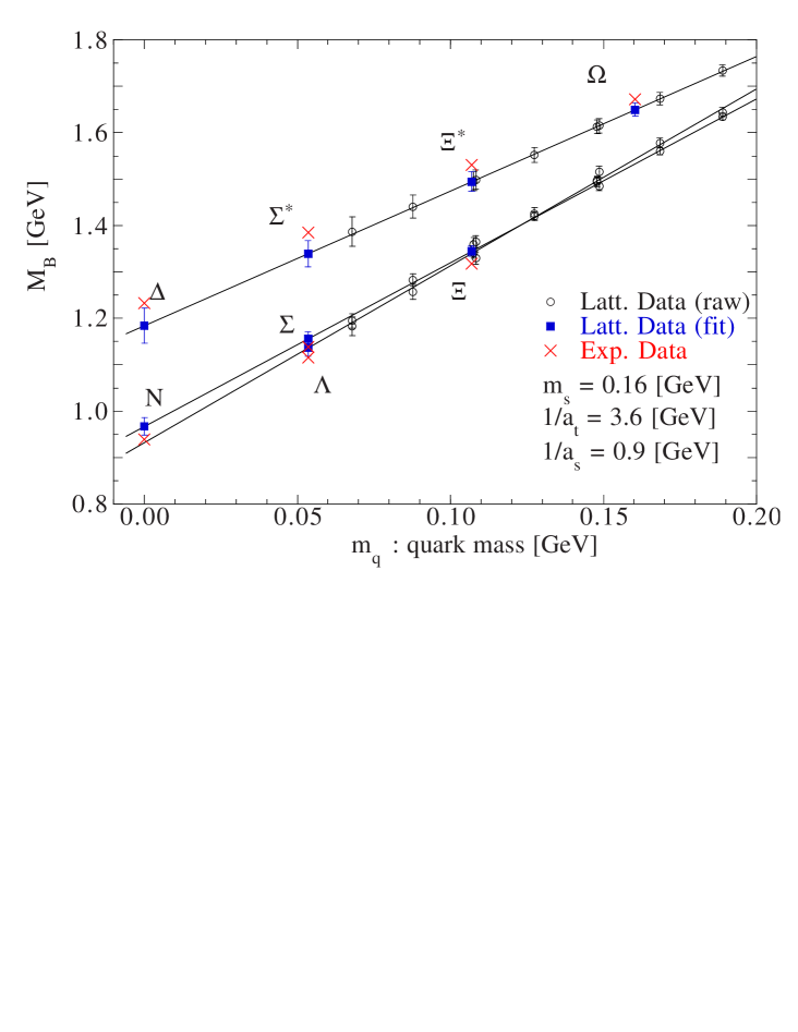
Figure 2: The spectra of octet and decuplet baryons with positive parity. The horizontal axis denotes the averaged current quark mass.

In our calculation, $u,d$ current quark masses are taken to be the same value as $m_{u}=m_{d}$ or $\kappa_{u}=\kappa_{d}$, and the strange current quark mass $m_{s}$ or $\kappa_{s}$ is taken to be an independent value. Then, the baryon masses are expressed as the function of $m_{u}$ and $m_{s}$ like $M_{B}(m_{u},m_{s})$, and therefore the baryon masses $M_{B}(m_{u},m_{s})$ are to be depicted on the $(m_{u},m_{s})$ plane. However, the lattice QCD result for the baryon masses $M_{B}$ seem to be well described as a function of the averaged current quark mass over the three quarks, $m_{q}=(m_{1}+m_{2}+m_{3})/3$, like $M_{B}(m_{q})$ in each channel. Therefore, we will use the simplified figures as the function of $m_{q}$, although the actual lattice QCD calculations are performed with different quark masses on $m_{u}(=m_{d})$ and $m_{s}$.

Let us start with the ground-state baryons shown in Figure 2, where the horizontal axis denotes the averaged current quark mass over the three quarks in the physical unit. We use the naive relation between the current quark mass and the hopping parameter as

$$m_{q}=\frac{1}{3}(m_{1}+m_{2}+m_{3}),\hskip 28.45274ptm_{i}=\frac{1}{2}\left(\frac{1}{\kappa_{i}}-\frac{1}{\kappa_{c}}\right).$$ (9)

The baryon masses are linearly extrapolated to the chiral limit, $m_{q}=0$. In the analysis of the baryon spectrum, we use the lattice scale determined by setting the averaged mass over the octet and the decuplet baryons at the chiral limit to the averaged mass of $N$ and $\Delta$. It results in $a_{\sigma}^{-1}=0.9$ GeV. The strange quark mass is determined so that the octet and the decuplet baryons in Fig. 2 globally reproduce the experimentally measured masses. Thus, for the strange quark, we adopt $\kappa_{s}=0.1229(1)$, which roughly corresponds to $m_{s}\simeq 0.16$ GeV as the current quark mass. This value seems consistent with the standard strange current-quark mass. Hereafter, we will fix $\kappa_{s}=0.1229(1)$ for the strange quark. Figure 2 shows that the lattice result reproduces that the measured baryon spectrum within 5 % deviation.

Octet-Decuplet mass splitting

Let us consider the difference of octet and decuplet baryon masses. This mass splitting monotonously decreases as the current quark mass increases. This tendency is consistent with the one-gluon-exchange explanation in the nonrelativistic quark model, assuming the constituent quark mass $M_{q}$ increases with the current quark mass $m_{q}$, as $M_{q}\simeq M_{0}+m_{q}$.

Figure 3: The positive and negative parity baryon masses in the flavor octet and singlet channels.

Negative parity baryons

Figure 3 shows the mass spectra of the flavor octet and singlet baryons with positive and negative parities as the function of the averaged current quark mass $m_{q}$. In each channel, the baryon mass spectrum shows clear linear behavior on the averaged current quark mass $m_{q}$ in the whole measured mass region. Then, we extrapolate the masses to the physical situation $m_{u}=m_{d}\simeq 0,m_{s}=0.16{\rm GeV}$, i.e., $m_{q}\simeq m_{s}/3$. One striking feature is that the singlet and octet negative parity baryons are almost degenerate. On the other hand, the lowest mass of the flavor-singlet positive-parity baryon is much larger than those in other channels. Extrapolating to the physical situation $m_{u}=m_{d}\simeq 0,m_{s}=0.16{\rm GeV}$ ($m_{q}\simeq m_{s}/3$), we obtain 1.6 GeV for the lowest mass of the flavor-singlet negative-parity baryon, which is described as a three quark state in the quenched lattice. Then, the experimentally observed negative-parity baryon $\Lambda(1405)$ is much lighter than the lowest mass of the flavor-singlet negative-parity baryon obtained in lattice QCD at the quenched level. Since the $q$-$\bar{q}$ pair creation is absent in the quenched QCD, this result implies that the simple three valence quark picture would not valid for $\Lambda(1405)$. One possible explanation is, as frequently suggested, that the $\Lambda(1405)$ is a mixture of a three quark state and an $N\bar{K}$ bound state. To clarify this subject, we are going to measure the $N\bar{K}$ state on the quenched lattice, where genuine bound state properties is apparent owing to the absence of the $q$-$\bar{q}$ pair creation.

4 Summary and outlook

In this paper, we report present status of our investigation of hadron properties using lattice QCD simulations. At this stage, systematic investigation of baryon spectrum is in progress at the quenched level. The result on the anisotropic lattice with $a_{\sigma}^{-1}\simeq 0.9$ GeV and anisotropy $\xi=4$ is as follows: (a) The octet-decuplet baryon mass splitting decreases with increasing current quark mass. This tendency is consistent with the one-gluon-exchange explanation in the constituent quark model. (b) The negative-parity baryons in octet and singlet channels are measured in good statistical precision. However, the experimentally observed negative-parity baryon $\Lambda(1405)$ seems much lighter than the lattice QCD result for the lowest mass of the SU(3) flavor-singlet negative-parity baryon. This may suggest the possibility of that $\Lambda(1405)$ is a mixture of the $N\bar{K}$ bound state and the three quark state. This would be clarified by successive lattice calculations for $qqq$-$q\bar{q}$ system in the quenched approximation.

Our present results have been carried out on rather course lattice. Hence, we need to perform the simulations on finer lattices to remove lattice artifacts. Then, the anisotropic lattice will be a powerful device to study detailed properties of hadrons including excited states, exotics and glueballs. The simulation with dynamical quarks are also to be performed.

Another course of our program is a comparison with the potential model analysis using the static quark potential extracted from lattice QCD. This will give us important information on the quark wave function and novel insight on the quark structure of hadrons.

We are grateful to Profs. Il-Tong Cheon and Su Houng Lee for their warm hospitality at Yonsei University. The lattice QCD simulations have been performed on NEC SX4 at Osaka University, and Hitachi SR8000 at KEK.

References

- [1] CP-PACS Collaboration (S.Aoki et al.), Phys. Rev. Lett. 84, 238 (2000).
- [2] For recent review, see e.g. S.Aoki, Nucl. Phys. B (Proc. Suppl.) 94, 3 (2001).
- [3] See also, H. Suganuma et al., these proceedings.
- [4] T.T. Takahashi, H. Suganuma, H. Matsufuru and Y. Nemoto, these proceedings.
- [5] N. Isgur and G. Karl, Phys. Rev. D 20, 1191 (1979).
- [6] M. Oka and K. Yazaki, Prog. Theor. Phys. 66, 556 (1981), ibid. 572.
- [7] S. Sasaki, T. Blum and S.Ohta, hep-lat/0102010, and references therein.
- [8] F. Karsch, Nucl. Phys. B205, 285 (1982).
- [9] T.R. Klassen, Nucl. Phys. B (Proc. Suppl.) 73, 918 (1999).
- [10] A. El-Khadra, A.S. Kronfeld and P.B. Mackenzie, Phys. Rev. D 55, 3933 (1997).
- [11] T. Umeda, R. Katayama, O. Miyamura and H. Matsufuru, hep-lat/0011085, to appear in Int. J. Mod. Phys. A.
- [12] J. Harada, A.S. Kronfeld, H. Matsufuru, N. Nakajima and T. Onogi, hep-lat/0103026.
- [13] T.R. Klassen, Nucl. Phys. B533, 557 (1998).