Topology and chiral symmetry breaking in SU($N_{c}$)
gauge theories
  

Abstract

We study the low-lying eigenmodes of the lattice overlap Dirac operator for SU$(N_{c})$ gauge theories with $N_{c}=2,3,4$ and 5 colours. We define a fermionic topological charge from the zero-modes of this operator and show that, as $N_{c}$ grows, any disagreement with the topological charge obtained by cooling the fields, becomes rapidly less likely. By examining the fields where there is a disagreement, we are able to show that the Dirac operator does not resolve instantons below a critical size of about $\rho\simeq 2.5a$, but resolves the larger, more physical instantons. We investigate the local chirality of the near-zero modes and how it changes as we go to larger $N_{c}$. We observe that the local chirality of these modes, which is prominent for SU(2) and SU(3), becomes rapidly weaker for larger $N_{c}$ and is consistent with disappearing entirely in the limit of $N_{c}=\infty$. We find that this is not due to the observed disappearance of small instantons at larger $N_{c}$.

I Introduction

The chiral symmetry of QCD is broken in several different ways. First, and most trivially, it is broken explicitly by modest quark mass terms. In addition the symmetry is broken spontaneously, leading to an octet of light pseudoscalars in the observed spectrum. If there were no quark mass terms these would be massless Goldstone bosons. However the flavour singlet $\eta^{\prime}$ is much too heavy to be a ‘near-Goldstone boson’, indicating that the associated U(1) axial symmetry is broken in some other way; and in fact it is known to be anomalous.

The SU(3) gauge fields of QCD possess non-trivial topological properties. In the semi-classical limit, on scales where one has analytic control, we know that the topology is localised in instantons. The anomaly is proportional to the topological charge density and one can show through an explicit calculation 'tHooft:1976fv:1986nc how instantons lead to a massive $\eta^{\prime}$. The mechanism relies on the existence of zero-modes of the Dirac operator in a background instanton field. While this provides a qualitative resolution of the U_A(1) problem, a complete quantitative calculation is still lacking.

In contrast to the anomalous breaking of the axial U(1) symmetry, there is no necessary involvement of topology in the spontaneous breaking of the remaining SU(3) chiral symmetry. Nonetheless it has long been speculated Caldi:1977rcCallan:1978gzCarlitz:1979yj that this might be so. A simple motivation starts with the observation Banks:1980yr that the chiral condensate is proportional to $\rho(\lambda=0)$, the (normalised) density of eigenvalues of the Dirac operator at zero eigenvalue. Now, we know that for a background field with topological charge $Q$ the Dirac operator will have (at least) $|Q|$ zero modes. These are however too few to contribute to the chiral condensate in the infinite volume limit, since a space-time volume $V$ will contain $O(V)$ topological charges of each sign and hence (if $\theta=0$) a net topological charge $Q\sim O(\surd V)$. However there will be $O(V)$ modes obtained through the mixing of what would have been zero modes if the $O(V)$ topological charges had zero overlap with each other. If this overlap is moderately small, the splitting from zero will be small and one would expect the resulting mode spectrum to have $\rho(\lambda=0)\not=0$, and hence to contribute to chiral symmetry breaking. This idea receives support from specific instanton model calculations Diakonov:1995eaSchafer:1998wv . (Indeed there is evidence that, in quenched QCD, $\rho(\lambda=0)$ is not just non-zero but may in fact be divergent Dowrick:1995wrSharan:1998gj:1998vp:1999mg .)

In practice, the topology of realistic gauge fields seems to be carried not only by well-separated instantons but also, and perhaps mainly, by larger heavily overlapping fluctuations which are much less tractable analytically. (See, for example, Smith:1998wt .) This should be no surprise in a theory with one length scale. Moreover there is a simple argument Witten:1979kh that isolated instantons will not survive the limit where the number of colours, $N_{c}$, becomes large: at fixed ’t Hooft coupling $g^{2}N_{c}$ 'tHooft:1974jz , the instanton weight includes a factor $\exp\{-8\pi^{2}/g^{2}\}=\exp\{-(8\pi^{2}/g^{2}N_{c})N_{c}\}$ which disappears exponentially with increasing $N_{c}$. This argument requires modification, but the conclusion that small isolated instantons do not survive the $N_{c}\to\infty$ limit appears to remain valid Teper:1980tq . On the other hand one believes that the chiral symmetry of QCD${}_{N_{c}=\infty}$ is spontaneously broken. While it is possible that the mechanisms for breaking chiral symmetry are different for $N_{c}=3$ and $N_{c}=\infty$, it would seem uneconomical of Nature to make use of such an option.

Whether topology drives part or all of the chiral symmetry breaking and, if so, whether the relevant topological fluctuations are approximately instanton-like, are clearly interesting questions and ones which it is natural to address by the simulation of the corresponding lattice field theories. Such calculations have long existed; for example in Hands:1990wc the spectrum of the Dirac operator in the SU(2) gauge theory is shown to have a non-zero density at $\lambda=0$, demonstrating the spontaneous breaking of the chiral symmetry. In addition it is shown that one loses this chiral symmetry breaking if one excludes eigenmodes that have a topological origin. Unfortunately this interesting conclusion, that topology does indeed drive chiral symmetry breaking, can be criticised because the staggered lattice fermions employed in Hands:1990wc suffer large lattice spacing corrections, particularly where topological zero modes are concerned. Until recently a similar criticism could be made of any of the lattice fermions in common use. However we now know that lattice fermions which satisfy the Ginsparg-Wilson relation, such as overlap fermions Narayanan:1993ss:1994sk:1995gwRandjbar-Daemi:1995sq:1995cq:1996mj:1997iz , domain wall fermions Kaplan:1992btShamir:1993zyFurman:1995ky or classically perfect fermions Hasenfratz:1994spWiese:1993cbDeGrand:1995ji:1995jk:1997ncHasenfratz:2000xz have good chiral properties and satisfy exact index theorems at finite lattice spacing. This opens the door to repeating the kind of calculation found in Hands:1990wc but now on a much sounder theoretical footing. The present work is in this spirit and adds to a number of recent papers on this topic Horvath:2001ir ; DeGrand:2000gq ; Hip:2001hcEdwards:2001ndDeGrand:2001wxGattringer:2001mn ; Horvath:2002gk .

With staggered fermions, lattice artifacts shift the exact topological zero modes away from zero and so when the would-be zero modes of neighbouring instantons and anti-instantons mix, the mixing is, in general, far from maximal. Thus, in practice, such mixed modes retain a substantial residual chirality, $\langle\psi|\gamma_{5}|\psi\rangle\not=0$, which can be used Hands:1990wc to identify the modes that possess a topological origin. With overlap lattice fermions, by contrast, the topological zero modes remain zero on the lattice, so the mixing is maximal and the chirality of non-zero modes is exactly zero, $\langle\psi|\gamma_{5}|\psi\rangle=0$, just as it is in the continuum. It is thus not so simple to determine the extent to which a $\lambda\not=0$ mode has a topological origin. If a mode is significantly influenced by an instanton of size $\rho$, centered at the space-time point $x$, then one would expect that the chiral density would be positive in the region of space-time, $v$, where the core of the instanton is located, i.e.

$$\int_{v}\psi^{\dagger}\gamma_{5}\psi\not=0.$$ (1)

More generally, the chiral density of $\psi$ should be non-zero in extended regions that match the locations of topological charges. Moreover the size of any such region should be related to the size of the corresponding topological charge and the sign of the chiral density should match the sign of that charge. The extent to which a nonzero mode can be described in this way determines the extent to which it can be said to possess a topological origin.

How to make quantitative such an analysis of the low-lying eigenmodes of the Dirac operator is not evident. A simple approach which has been used in much of the recent literature Horvath:2001ir ; DeGrand:2000gq ; Hip:2001hcEdwards:2001ndDeGrand:2001wxGattringer:2001mn ; Horvath:2002gk focuses on the lattice sites at which the eigenmode is large (using some reasonable cut-off) and asks how chiral the mode is at those sites. Qualitatively, the more chiral it is, the more likely it is to have a topological origin. A recently popular measure Horvath:2001ir ; DeGrand:2000gq ; Hip:2001hcEdwards:2001ndDeGrand:2001wxGattringer:2001mn ; Horvath:2002gk is given by the quantity $X(x)$ Horvath:2001ir defined via the ratio of the positive and negative chiral densities $\psi_{\uparrow}^{\dagger}\psi_{\uparrow}$ and $\psi_{\downarrow}^{\dagger}\psi_{\downarrow}$ at the point $x$ through

$$\tan\left(\frac{\pi}{4}(1+X(x))\right)=\biggl{(}\frac{\psi_{\downarrow}^{\dagger}\psi_{\downarrow}}{\psi_{\uparrow}^{\dagger}\psi_{\uparrow}}\biggr{)}^{1/2}\,.$$ (2)

In this paper we shall present our results for this quantity, and for some physically motivated variants, not only for the SU(3) gauge theory considered in Horvath:2001ir ; DeGrand:2000gq ; Hip:2001hcEdwards:2001ndDeGrand:2001wxGattringer:2001mn ; Horvath:2002gk but also for the SU(2), SU(4) and SU(5) gauge theories. In this way we can simultaneously address the interesting question of what happens as $N_{c}\to\infty$.

A more sophisticated approach is to write a non-zero mode, $\psi$, as a linear combination of the would-be zero modes, $\psi^{0}_{I}$, associated with the (anti)instantons, $I$, in the background gauge field under consideration

$$\psi=\sum_{I}c_{I}\psi^{0}_{I}+\delta\psi.$$ (3)

Such an approach has been pursued in DeGrand:2000gq using the semi-classical form of $\psi^{0}_{I}$ and a particular algorithm to determine the topological charges in the gauge field. Clearly there are ambiguities here both to do with what to use for $\psi^{0}_{I}$ and how to determine the topological structure of the gauge field. Our (ongoing) work on this approach will be reported upon in another publication.

In addressing these questions one needs to know how the locality properties of the overlap Dirac operator Hernandez:1998et affects its ability to resolve the topological structure on typical lattice gauge fields. Ideally one would like the situation to be that the overlap operator possesses zero modes for topological charges with sizes (in lattice units) $\rho\geq\rho_{c}$ where $\rho_{c}$ is small enough that reliable calculations are accessible in practice. Because typical SU(2) and SU(3) gauge fields contain a substantial number of small instantons, it has not been easy to establish whether this is the case or not. In typical SU(4) and SU(5) fields, by contrast, narrow topological charges are rare and it becomes possible to address this question with much less ambiguity. We shall be able to show explicitly that the ideal scenario described above, is what actually occurs.

The calculations we perform involve a quark propagating in the vacuum of an SU($N_{c}$) gauge theory rather than in the vacuum of full QCD with $n_{f}\neq 0$ flavours and $N_{c}$ colours. It is interesting to note, however, that for any non-zero quark mass the $N_{c}\to\infty$ limit of quenched QCD is precisely the $N_{c}\to\infty$ limit of full QCD. Thus any statements we are able to make about the former apply to the latter as well.

The paper is organised as follows. In section II we present the setup of our lattice calculation and we give some technical details concerning the implementation of the chirally symmetric overlap lattice Dirac operator. Section III contains the results of the calculation. It is divided into several subsections where we discuss the results for topology, local chirality, correlation functions and instanton size distributions. A summary and conclusions follow in section IV.

II Setup

The explicit form of the standard massless overlap Dirac operator reads Neuberger:1998fp

$$D(0)=\frac{1}{2}(1+\gamma_{5}\text{sgn}(H_{\text{W}}(m)),$$ (4)

where $H_{\text{W}}(m)$ denotes the hermitian Wilson-Dirac operator $\gamma_{5}D_{\text{W}}(m)$ with its mass parameter $m=-1$ in the supercritical mass region. Since $H^{2}(0)=D^{\dagger}(0)D(0)$ commutes with $\gamma_{5}$ we can find eigenmodes of $H^{2}(0)$ with definite chirality Edwards:1998yw :

$$H^{2}(0)\psi_{\uparrow,\downarrow}=\lambda^{2}\psi_{\uparrow,\downarrow},\quad\gamma_{5}\psi_{\uparrow,\downarrow}=\pm\psi_{\uparrow,\downarrow}\,.$$ (5)

The non-zero eigenmodes of $H^{2}(0)$ with $0<\lambda<1$ are doubly degenerate with opposite chirality and the non-zero eigenmodes of $D(0)$ can be obtained as

$$\psi_{\pm}=\frac{1}{\sqrt{2}}\left(\psi_{\uparrow}\pm i\psi_{\downarrow}\right)$$ (6)

with eigenvalues

$$\lambda_{\pm}=\lambda^{2}\pm i\sqrt{\lambda^{2}(1-\lambda^{2})}\,.$$ (7)

In the following we count such an eigenmode pair as one mode.

The overlap Dirac operator possesses exact zero modes with $\lambda=0$ that are stable under small perturbations of the background gauge field. They are used in the definition of the fermionic topological charge $Q_{f}$ via the index of the overlap Dirac operator, i.e.,

$$Q_{f}\equiv n_{+}-n_{-},$$ (8)

where $n_{\pm}$ counts the number of zero modes with positive and negative chirality, respectively.

The local chirality parameter is equal for the two related modes $\psi_{+}$ and $\psi_{-}$ and can be calculated via the ratio of the positive and negative chiral densities, cf. eq. (2). For the exact zero modes we obviously have $X(x)=\pm 1$ according to their chirality.

We generated ensembles of gauge field configurations on $12^{4}$ lattices using the pure gauge Wilson action with four different numbers of colours $N_{c}=2,3,4$ and 5 at a fixed lattice spacing $a\simeq 0.12$ fm set by the string tension $a\sqrt{\sigma}=0.261$ from Lucini:2001ej . This corresponds to a physical volume $V\simeq 4.3\,\text{fm}^{4}$. The configurations are separated by 1000 update sweeps. The simulation parameters are collected in Table 1.

$N_{c}$	$\beta$	conf.
2	12.40	30
3	15.90	50
4	10.84	30
5	17.16	30

Table 1: Simulation parameters for the ensembles of gauge field configurations on $12^{4}$ lattices. The $\beta$-values are interpolated to match a fixed lattice spacing $a\simeq 0.12$ fm set by the string tension $a\sqrt{\sigma}=0.261$ from Lucini:2001ej . The number of colours, $N_{c}$, the values of $\beta$ and the number of generated configurations are given.

It is clear that setting the scale by the string tension is not unique and there are other sensible ways to determine the scale in different theories. Moreover, the interpolation which is needed for extracting the $\beta$-values to match the physical scale introduces an additional ambiguity. In order to assess these kind of uncertainties in the scale we use the mass of the $2^{++}$ glueball to set the lattice spacing for the different gauge groups instead of the string tension. We use the $2^{++}$ rather than the $0^{++}$ glueball mass because the latter suffers from large lattice corrections which are quite different for the different gauge groups. This is due to the different sensibility to the strong-to-weak coupling crossover at finite lattice spacing. For the $\beta$-values quoted in table 1 we obtain interpolated $2^{++}$ glueball masses of $am_{2^{++}}=1.34(4)$ for SU(5) and $am_{2^{++}}=1.33(5)$ for SU(4) which has to be compared to the directly measured $am_{2^{++}}=1.30(4)$ for SU(3) Lucini:2001ej . On the other hand, for SU(2) we obtain $am_{2^{++}}=1.41(5)$ from an interpolation and $am_{2^{++}}=1.50(5)$ from a direct measurement Lucini:2001ej . So, for SU(2) the uncertainty in the lattice spacing is quite substantial while for SU(4) and SU(5) it is completely negligible.

We then calculated all the eigenmodes $\psi_{\uparrow,\downarrow}$ of $H^{2}(0)$ with $\lambda^{2}<0.1$ using the Ritz functional algorithm of Kalkreuter:1996mm . The cut-off amounts to $\text{Im}\lambda_{\pm}<0.3$ and corresponds roughly to a physical value of $520\,\text{MeV}$. The average number of modes per configuration we found below this cut-off (including zero modes) was 6.63(14), 5.46(11), 5.37(13) and 5.17(13) for $N_{c}=2,3,4$ and 5, respectively. The eigenmodes were computed to an accuracy for which the gradient $g$ of the Ritz functional had $|g|<10^{-5}$.

In order to speed up the whole calculation we applied the following two standard methods. Firstly, by working in a given chiral sector where all vectors $b_{\pm}$ obey $\gamma_{5}b_{\pm}=\pm b_{\pm}$ one can write Edwards:1998wx

$$H(0)^{2}b_{\pm}=\frac{1}{2}(1\pm\frac{1}{2}(1\pm\gamma_{5})\text{sgn}(H_{\text{W}}(m)))b_{\pm}\,.$$ (9)

One application of $H(0)^{2}$ on a vector $b_{\pm}$ therefore requires only one application of the sign-function. Secondly, we calculated the 15 lowest eigenmodes of $H_{\text{W}}(m)$ to an accuracy of $|g|<10^{-8}$ and treated the 15 lowest ones exactly by first projecting them out of $b_{\pm}$ and adding their contribution to the sign-function analytically. The 16-th lowest and the highest eigenvalue of $H_{\text{W}}(m)$ were used to define the interval over which we approximated the sign-function using Legendre polynomials Bunk:1998wj .

The reason for employing Legendre polynomial approximations rather than rational approximations was twofold. Firstly, it enabled us to use a ’dynamical’ accuracy for the sign-function, i.e. we could easily change the accuracy of the approximation during the course of calculating the eigenvectors. To be more precise, we started with a low order approximation of the sign-function at the beginning of an eigenvector calculation and increased the order successively so as to have the error of the sign-function applied on the search vector in the Ritz-functional always $10^{-2}$ times smaller than the gradient of the search vector. For the application of the sign-function on the eigenvector itself we chose a higher order approximation in order to avoid destabilisation of the procedure.

In this way we could manage to bring down the number of $H_{\text{W}}(m)^{2}$ multiplications per sgn-function application on a search vector, e.g. for SU(2) to around 50.

Secondly, it turned out that the three term recursion relation inherent in the Legendre polynomial approximation is much more economic with respect to the required computer resources than the multi-shift solver used for the partial fraction expansion of the rational function approximation. As a consequence we found that the Legendre polynomial approximation ran roughly two times faster than the rational function approximation on our Alpha/Linux workstations even when the converged systems were removed from the multi-shift solver. We ascribe this fact to the large memory requirement of the multi-shift solver resulting in a substantially worse performance. In principle the large memory requirement can be partially avoided by resorting to a double pass multi-shift solver Neuberger:1998jk , however, we did not employ this variant here.

These two observations in favour of the Legendre polynomials apply equally well to Chebysheff polynomials. Moreover, the latter allow polynomial approximations which are optimal with respect to the uniform norm and are regarded to be superior to Legendre polynomial approximations. For all practical purposes, i.e. counting the number of $H_{\text{W}}$ applications, it turns out that the difference between Chebysheff and Legendre polynomials are negligible.

Finally we note that our implementation is based on the QCDF90-package Dasgupta:1996nj .

III Results

III.1 Topology

Since the overlap Dirac operator possesses exact zero modes we can use its index, via equation (8), to obtain the total topological charge of the background gauge field. We shall refer to this as the fermionic topological charge $Q_{f}$. In table 2 we list our results for the expectation values of various quantities involving $Q_{f}$ for the different $N_{c}$ ensembles. Since our ensembles are small, the statistical errors are large, but it is already clear that the topological susceptibility $\chi_{t}$, when expressed in units of the string tension $\sigma$, varies little with $N_{c}$. This confirms similar claims made using other methods Lucini:2001ej .

$N_{c}$	$\langle Q_{f}\rangle$	$\langle|Q_{f}|\rangle$	$\langle Q_{f}^{2}\rangle-\langle Q_{f}\rangle^{2}$	$\chi_{t}/\sigma^{2}$	$\langle Q_{g}^{2}\rangle-\langle Q_{g}\rangle^{2}$	$\langle(Q_{f}-Q_{g})^{2}\rangle/\langle Q_{f}^{2}\rangle$
2	0.13(29)	1.20(19)	2.52(63)	0.0261(65)	2.49(51)	0.318(69)
3	0.08(21)	1.08(14)	2.03(51)	0.0211(53)	2.36(49)	0.314(70)
4	0.23(25)	1.17(16)	2.05(45)	0.0213(47)	2.36(52)	0.079(33)
5	0.53(28)	1.27(17)	2.25(49)	0.0234(51)	2.45(57)	0.039(22)

Table 2: Expectation values of the fermionic topological charge, its modulus and variance and the topological susceptibility in units of the string tension as well as the variance of the gluonic topological charge. The last column provides a measure of the violation of the index theorem.

An important question, which we shall now address, is how reliable is the index theorem for these particular lattice ensembles. As with any measure of the topology of lattice gauge fields there must be ambiguities. For example, if we have a smooth lattice gauge field containing a single instanton whose size is much greater than the lattice spacing, $\rho\gg a$, then any reasonable measure of topology should assign the field $Q=1$. We can now smoothly shrink the instanton and eventually we will have $\rho\ll a$. If the instanton is centered well within a lattice hypercube then the link gauge fields will now be those corresponding to a gauge singularity and the same reasonable measure of topology must assign the field $Q=0$. So for any measure of lattice topology there will be some critical value of the size, $\rho_{c}$, at which its value will change from $Q=1$ to $Q=0$. We would like $\rho_{c}$ to be large enough that it excludes any very small instanton with $\rho\sim a$ whose action is grossly distorted from its continuum value by the lattice discretisation, yet small enough that it does not exclude larger continuum-like instantons. As $a\to 0$ the latter requirement is achieved automatically since the usual $\exp\{-8\pi^{2}/g^{2}(\rho)\}$ factor suppresses very small instantons for any SU$(N_{c})$ gauge theory. What happens in our case, where $a\simeq 0.26/\surd\sigma\simeq 0.12$ fm, is a question we shall address in this section.

We also remark that in the case of the overlap Dirac operator, an explicit ambiguity arises from the fact that when one varies the mass parameter $m$ within its theoretically acceptable range, a mode of $H_{\text{W}}(m)$ will occasionally change sign, thus changing the operator index Edwards:1999bm . This creates a corresponding ambiguity in the value of $Q_{f}$ to be assigned to the underlying gauge field.

The extent and nature of all these ambiguities will not only affect the value of $\chi_{t}$ in table 2 , but will also affect any attempt to investigate the topological content of the non-zero but low-lying modes that drive chiral symmetry breaking.

Ideally, and optimistically, one would like the situation to be the following. For the overlap Dirac operator we would like to have $\rho_{c}\sim 2a$ so that it is large enough to exclude lattice ‘dislocations’ yet small enough to have a minimal impact on physical topology. The ambiguity in the choice of $m$ should simply reflect the fact that $\rho_{c}$ varies with $m$, but this variation should be weak enough that for any reasonable choice of $m$, the value of $\rho_{c}(m)$ continues to be as described above. That is to say, the mode crossing of $H_{\text{W}}(m)$ with $m$, should involve very small instantons which are at the margin of being resolved by the overlap Dirac operator: for some values of $m$ they are resolved and give $Q_{f}=1$ while for other values of $m$ they remain unresolved and contribute $Q_{f}=0$. We shall now provide some evidence that this optimistic scenario is indeed the case.

What places us in a position to address these questions is that as $N_{c}$ grows, the continuum density of small instantons is rapidly suppressed Lucini:2001ej . Thus most of our SU(4) and SU(5) lattice field configurations do not contain any small instantons at all; and where they do, they usually only contain one. Thus if there is a correlation between small instantons and the ambiguities in the overlap index, it should be easy to see. In SU(3) by contrast, the fields frequently possess several small instantons and patterns are much harder to discern.

In order to determine something about the topological charge content of the lattice gauge fields, we analyse them using a standard cooling technique Hoek:1987ndTeper:1999wp . This method also has its ambiguities but these are reasonably well understood. We now sketch the method and summarise its uncertainties.

To cool a given rough lattice gauge field we perform a sequence of sweeps through the lattice, always choosing the new link matrices so as to minimise the plaquette action. After each sweep we calculate the lattice topological charge density $Q_{g}(x)$ using a simple lattice version of the continuum $F\widetilde{F}$ operator. The sum of this charge density over the lattice gives us a measure of $Q$ that we label $Q_{g}$. In principle this depends on the number of cooling sweeps. In practice, after a very few such sweeps, the fields become smooth enough that $Q_{g}$ becomes independent of the cooling. This is not quite true: an instanton will (usually) slowly shrink under cooling and will eventually shrink out of the lattice. However such a narrowing instanton produces a prominent $\propto 1/\rho^{4}$ peak in $Q_{g}(x)$ which is easy to monitor and its disappearance within a hypercube is accompanied by characteristic signals. We monitor peaks in $Q_{g}(x)$ (and also in the action density) so that we are able to unambiguously detect the disappearance of any topological charge after about 4 cooling sweeps. Since a few cooling sweeps cannot undo coherent long-range structures in the fields (any more than a few Monte Carlo sweeps can create them) or indeed to change their size by a large amount, we expect that the sizes of the instantons after a few cooling sweeps, are closely related to their sizes in the original uncooled fields. This relationship is however only qualitative, since what happens to an individual instanton depends on its environment. For example, a narrow instanton would normally shrink under cooling. However if it is overlapping strongly with an anti-instanton it might well grow in size instead (so that the two opposite charges can more readily annihilate). Occasionally, if the environment is extreme, one can see that the size increases quite rapidly with cooling.

We shall make the choice of 10 cooling sweeps at which to analyse the topological structure. From the peaks in $Q_{g}(x)$ we can extract an instanton size $\rho$ using the continuum formula $Q_{peak}=6/\pi^{2}\rho^{4}$ (see also the more detailed discussion in section III.4). This is obviously approximate and can be partially corrected for discretisation effects. However we shall not do so here since we are only aiming at uncovering qualitative features. If $\rho$ is small then the peak is large and its identification is unambiguous. For large $\rho$, by contrast, the peak is very small and could be a remnant of the roughness of the original fields. Thus any attempt to identify individual large instantons is not reliable. Instantons that are small after 10 cooling sweeps will usually correspond to instantons that were small in the original uncooled fields. However, as explained above, this will only usually be the case.

The total topological charge $Q_{g}$ should, of course, be an integer but, because of discretisation effects, the sum of $Q_{g}(x)$ will not be. Accordingly we transform this sum to the appropriate nearby integer value. Occasionally it is not evident which integer is appropriate, and in that case it suffices to note the charges of those instantons that are smallest, and therefore suffer the largest lattice corrections, and correct the value of $Q_{g}$ accordingly. (One can finesse this step by using improved lattice topological charge operators which give values of $Q_{g}$ very close to an integer. See Bilson-Thompson:2001ca for a recent discussion.)

Thus the above cooling procedure gives us an integer topological charge $Q_{g}$ and also some detailed information on the smaller instantons. Cooling does not, however, provide us with any information on ‘dislocations’ – fields with $\rho\sim a$ which are close to the $Q=0,1$ boundary and whose action is typically far from the continuum action – since, as one would expect, these appear to be erased in the first one or two cooling sweeps, i.e. before the topological charge density has become smooth enough for topological charges to be identifiable. The density of these dislocations depends on the action used. That such dislocations can be numerous has been confirmed in SU(2) calculations with the plaquette action Pugh:1989qd:1989ek using a geometric definition of $Q$ Phillips:1986qd . Such dislocations are present in small volumes that do not contain any real physical instantons, and one sees explicitly Pugh:1989qd:1989ek by cooling such configurations that dislocations immediately disappear.

We now turn to a comparison between the topological charge $Q_{g}$ that one obtains by cooling and the fermionic topological charge $Q_{f}$. In figure 1 we compare the values of $Q_{f}$ and $Q_{g}$ as obtained for each gauge field ensemble . (For presentational purposes, the values of $Q_{g}$ shown here are prior to any adjustment to integer values, so that the points corresponding to different lattice fields can be distinguished from each other.) We see a dramatic change between these ensembles. For SU$(2)$ the differences are frequent even if a marked correlation is evident. For SU$(5)$ it has become rare for the charges not to be in agreement.

Figure 1: The gluonic field theoretic topological charge $Q_{g}$ after 10 cooling sweeps vs. the fermionic topological charge $Q_{f}=n_{+}-n_{-}$ for $N_{c}=2,3,4$ and 5.

To make the comparison more quantitative we calculate the quantity $\langle(Q_{f}-Q_{g})^{2}\rangle$ and plot it as a function of $N_{c}$ in figure 2 together with the values of $\langle Q_{f}^{2}\rangle$ and $\langle Q_{g}^{2}\rangle$. (In fact we plot $\langle Q^{2}\rangle-{\langle Q\rangle}^{2}$ in the latter two cases. Of course the fact that $\langle Q\rangle\not=0$ is an artifact of our low statistics and happens to be only significant in the case of SU$(5)$.) If the charges were uncorrelated, i.e. $\langle Q_{f}Q_{g}\rangle=0$, then we would expect to find $\langle(Q_{f}-Q_{g})^{2}\rangle=\langle Q_{f}^{2}\rangle+\langle Q_{g}^{2}\rangle$. From the values plotted in figure 2 (cf. also table 2) it is clear that the correlation is strong even for SU(2), and rapidly increases as $N_{c}$ increases. We also note that the susceptibility, when expressed in physical units as $\chi_{t}/\sigma^{2}$, is independent of $N_{c}$ within our errors.

Figure 2: $\langle Q_{f}^{2}\rangle-{\langle Q_{f}\rangle}^{2}$ (circles), $\langle Q_{g}^{2}\rangle-{\langle Q_{g}\rangle}^{2}$ (squares) and $\langle(Q_{f}-Q_{g})^{2}\rangle$ (diamonds) as a function of $N_{c}$.

The fact that disagreement between $Q_{f}$ and $Q_{g}$ becomes rare for SU(4) and SU(5), provides us with an opportunity to determine the reason for such disagreements. We turn to this now.

As $N_{c}$ increases, a striking change is the rapid disappearance of small instantons. This is a simple consequence of the $N_{c}$ dependence of the $\exp\{-8\pi^{2}/g^{2}(\rho)\}$ factor that dominates the weight of small (and therefore approximately ‘dilute’) instantons. It has been explicitly observed in the high statistics calculations of Lucini:2001ej and we will confirm it through a somewhat different analysis later on in this paper (see section III.4). We know that cooling will remove very small instantons, but the SU(2) instanton size distribution Lucini:2001ej tells us that this must be confined to instantons with $\rho<2a$. Thus the suppression we observe for increasing $N_{c}$ at larger $\rho$ must indeed be a dynamical effect.

So, as we increase $N_{c}$ small instantons are suppressed and so is any disagreement between $Q_{f}$ and $Q_{g}$. It is natural to ask if these two phenomena are related. To address this question we take each of our lattice fields after 10 cooling sweeps, find the maximum value of the topological charge density, $\max_{x}|Q_{g}(x)|$, and label by $Q_{\text{max}}$ the corresponding value of $Q_{g}(x)$. If the reason for $Q_{f}\not=Q_{g}$ is that the overlap fermionic operator does not resolve small instantons, then we would expect that plotting $\Delta Q\equiv Q_{f}-Q_{g}$ and $Q_{\text{max}}$ for each field configuration will show that $\Delta Q\not=0$ is associated with a large value of $Q_{\text{max}}$ and, in addition, that the sign of $\Delta Q$ should be the same as that of $-Q_{\text{max}}$. We display such plots in figure 3 for SU(4) and SU(5) respectively. We observe that in the case of SU(5) $\Delta Q\not=0$ is always associated with a very large value of $|Q_{\text{max}}|$ and that the sign of $\Delta Q$ is indeed the same as that of $-Q_{\text{max}}$. In SU(4) that is also the case, except for one configuration where $|Q_{\text{max}}|$ is not very large although the sign matches $\Delta Q$. As we remarked earlier, occasionally a narrow instanton broadens rapidly under cooling and indeed there is evidence from the earlier cooling history of this particular field configuration that this is what has happened here. However rather than appeal to such a much more complicated analysis, we prefer to maintain our simpler analysis, and simply accept occasional mismatches as being consistent with the expected frequency of such effects.

Figure 3: Comparison of the maximum peak value $-Q_{\text{max}}$ (empty circles) with the difference between the fermionic and field theoretic topological charge $\Delta Q=Q_{f}-Q_{g}$ (filled circles) for $N_{c}=5$ and 4. Note that $Q_{\text{max}}$ is rescaled to facilitate comparison. Monte Carlo (MC) time is in units of $10^{3}$ sweeps.

What helps to make these simple plots so compelling is that small instantons are rare in SU(4) and SU(5), so that if one of our lattice fields has one such small instanton it is unlikely to have a second one as well. Otherwise one could frequently have cancellations, and hence $\Delta Q=0$, undermining any simple visual inspection of the kind that suffices here. In SU(3), by contrast, there are more small instantons and things are indeed considerably more complex, as we see from figure 4. Nonetheless even here careful scrutiny of the figure will largely confirm what we have seen in the cases of SU(4) and SU(5).

Figure 4: Same as figure 3 but for $N_{c}=3$.

We believe that all this provides convincing evidence that the overlap Dirac operator resolves all topological charges with, roughly, $\rho\geq 2.5a$ – and perhaps a little less than that. This means that for reasonably small $a$ the operator will resolve all the physical instantons and, at the same time, will exclude all the unphysical (near-)dislocations.

We remarked earlier that an explicit ambiguity in $Q_{f}$ arises from the fact that when we vary the $m$ of $H_{\text{W}}(m)$ in equation (4) within the supercritical mass region, eigenvalues of $H_{\text{W}}(m)$ will sometimes change sign, at which point $Q_{f}$ will change. (All this for a given gauge field.) Is there any evidence for our earlier suggestion that the mode that changes sign may be associated with a very narrow instanton which is resolved by the overlap Dirac operator for one range of $m$ and not for another? To address this question directly one needs to vary $m$ which we have not done in our calculations. However one can go some way following an indirect line of reasoning. If a mode of $H_{\text{W}}(m)$ passes through zero at some value of $m$, then the mode will be very small at nearby values of $m$. Thus we would expect the modes at $m=-1$ to be smaller, on the average, if we are examining a field configuration for which there are modes that change sign at a value of $m$ close to $m=-1$. So we can ask whether fields with small instantons have smaller modes of $H_{\text{W}}(m=-1)$ than fields without such small charges. We show the results of such an exercise for SU(5) in figure 5.

Figure 5: The smallest eigenvalue of the hermitian Wilson Dirac operator $\lambda_{\text{min}}(H_{\text{W}}^{2})$ for each field configuration in the $N_{c}=5$ ensemble against the value of $|Q_{\text{max}}|$ defined in the text.

Here we plot the value of the smallest non-zero eigenvalue $\lambda_{\text{min}}$ of $H_{\text{W}}(m=-1)^{2}$ for each field against the value of $|Q_{\text{max}}|$ defined earlier. We see from figure 5 that there is a significant trend for field configurations with smaller instantons to be more likely to have unusually small modes of $H_{\text{W}}(m=-1)$. This provides some significant evidence that small instantons are indeed the cause of this ambiguity. We also note that there is some evidence that $\lambda_{\text{min}}$ actually has a minimum at $|Q_{\text{max}}|\simeq 0.015$ and then increases again for the narrower instantons that correspond to larger $|Q_{\text{max}}|$. This fits our picture: the very smallest instantons are invisible for any reasonable value of $m$ and so will not involve level crossings near $m=-1$. The position of the minimum suggests that the critical instanton size visible to the overlap operator is $\rho_{c}\simeq 2.5a$. Finally we would like to emphasise again that we owe the possibility of the above argument entirely to the fact that the SU(5) (and also the SU(4)) gauge field configurations are much ’cleaner’ than the ones for SU(3) or SU(2) in the sense that small instantons are much rarer and usually unaccompanied by other small instantons in the configuration. As a consequence it is no surprise that the trend observed in figure 5 is less pronounced in an equivalent plot for SU(4) and almost completely distorted and obscured for SU(3) and SU(2).

More evidence for the smoothness of the gauge fields at larger $N_{c}$ is provided by figure 6.

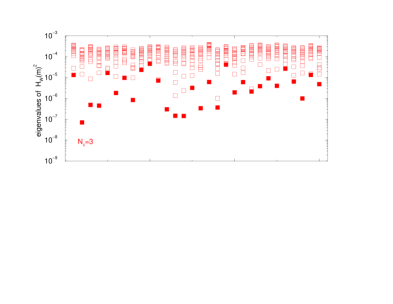
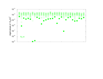
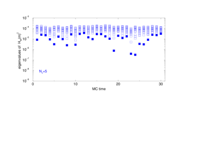
Figure 6: The 15 lowest lying eigenvalues of $H_{\text{W}}(m)^{2}$ with $m=-1$ for $N_{c}=2,3,4$ and 5. Monte Carlo (MC) time is in units of $10^{3}$ sweeps. In the case of $N_{c}=3$ we only show the eigenvalues of configurations 11 to 40 for ease of comparison.

Here we plot the lowest 15 eigenvalues of $H_{\text{W}}(m)^{2}$ with $m=-1$ as a function of Monte Carlo (MC) time. We clearly observe a trend for larger $N_{c}$ field configurations to have less but more isolated unusually small eigenvalues. In addition the lower bound of the bulk of eigenvalues seems to be much more rigid for SU(5) and SU(4) than it is for SU(3) or even SU(2). Another observation which is evident from just a visual inspection of the plots, is that the density of small eigenvalues in the bulk grows with increasing $N_{c}$ just as one would expect. This is, however, in contrast to what we observe for the density of small eigenvalues of the overlap operator $D(0)$ (see section II). There we found that the number of eigenvalues below the cut-off $\lambda^{2}<0.1$ shows a tendency to decrease with increasing $N_{c}$. Although one expects the spectrum of the Dirac operator at small eigenvalues to remain the same for increasing $N_{c}$ the scale of the eigenvalue distribution is governed by the quark condensate growing linearly with $N_{c}$ and thus the spacing of the eigenvalues should become smaller when expressed in terms of the mass of a bound state (or the string tension).

III.2 Local chirality

After the discussion on how the overlap Dirac operator resolves the total topological charge and how that compares to a standard analysis using cooled gauge fields, we would now like to address the question how the low lying modes of the overlap Dirac operator are affected by topology. As discussed in the introduction one possible approach is to investigate the local chirality parameter $X(x)$ defined via the ratio of the positive and negative chiral densities of the eigenmodes, cf. eq. (2). One can then determine from the distribution of $X(x)$ for separate eigenmodes (or ensembles thereof) how chiral they are and so how likely they are to have their origin in the mixing of zero modes.

In figure 7 and 8 we show the results of such a calculation. For each eigenmode we identify a volume fraction $f_{V}$ of the lattice sites for which the wave function density $\psi^{\dagger}\psi(x)$ is largest and include the corresponding value $X(x)$ in the distribution. Figure 7 shows the local chirality probability distributions $P(X)$ at a volume fraction $f_{V}=1.0\%$ (left plots) and $f_{V}=2.0\%$ (right plots), while figure 8 shows the probability distributions for $f_{V}=6.25\%$ (left plots) and $f_{V}=12.5\%$ (right plots). In both figures the upper plots include all the non-zero eigenmodes with $\lambda^{2}<0.03$ and the lower plots the ones with $\lambda^{2}<0.1$, respectively. In order to make the plots more clear we symmetrise the probability distributions $P(X)$ in all cases, i.e. $P(-X)=P(X)=1/2(\tilde{P}(X)+\tilde{P}(-X))$ where $\tilde{P}(X)$ is the original unsymmetrised distribution.

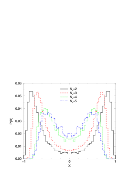
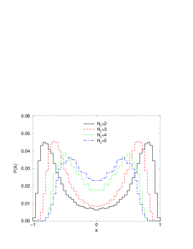
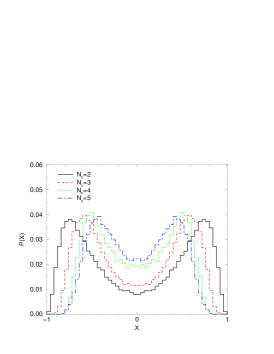
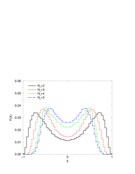
Figure 7: Local chirality histograms for the lowest non-zero modes of the overlap Dirac operator with $\lambda^{2}<0.03$ (top) and $\lambda^{2}<0.1$ (bottom) at a volume fraction $f_{V}=1.0\%$ (left column) and $f_{V}=2.0\%$ (right column) of sites with the largest wave function density $\psi^{\dagger}\psi(x)$.

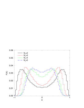
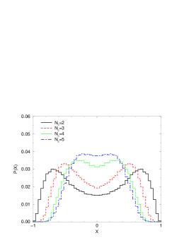
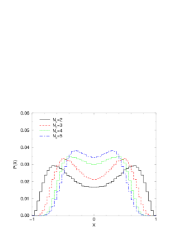
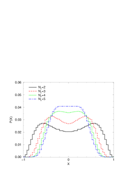
Figure 8: Local chirality histograms for the lowest non-zero modes of the overlap Dirac operator with $\lambda^{2}<0.03$ (top) and $\lambda^{2}<0.1$ (bottom) at a volume fraction $f_{V}=6.25\%$ (left column) and $f_{V}=12.5\%$ (right column) of lattice sites with the largest wave function density $\psi^{\dagger}\psi(x)$.

In the upper plots of figure 7 a clear double peak structure is visible for all the gauge groups we studied. Thus the lowest non-zero eigenmodes of the overlap Dirac operator appear to be chiral in their peaks, however, this is less pronounced as $N_{c}$ increases. As we include more and more non-zero modes while keeping $f_{V}$ fixed, cf. lower plots in figure 7, the double peaking becomes slightly weaker, but the modes appear still rather chiral in their peaks. The weakening is most evident for SU(2) and becomes gradually less apparent with increasing $N_{c}$. This suggests that for SU(2) and SU(3) the non-zero eigenmodes become less chiral, as the modes are lifted away from zero, while for SU(4) and SU(5) the modes below $\lambda^{2}<0.1$ appear to be all similarly (but more weakly) chiral in their peaks.

Of course one might object that comparing the distributions at a fixed volume fraction $f_{V}$ is not the most sensible approach since it does not take into account how big a fraction $f_{W}$ of the total wave function density is considered. In order to assess this issue we calculate for each volume fraction $f_{V}$ the corresponding contribution to the total wave function. In table 3 we collect the wave function fraction $f_{W}$ for each ensemble of gauge fields as a function of $f_{V}$ for all non-zero modes with $\lambda^{2}<0.1$. We observe that for any given $f_{V}$ we account for less and less of the total wave function as we increase $N_{c}$. In fact, the ratio $f_{W}/f_{V}$ in the limit $f_{V}\rightarrow 0$, i.e. the derivative of $f_{W}$ with respect to $f_{V}$ at $f_{V}=0$, can serve as a measure of the smoothness or locality of the eigenmodes. It is obvious from table 3 that the non-zero eigenmodes become less localised with increasing $N_{c}$ and one should keep that in mind when comparing the chirality distributions at a fixed volume fraction.

Since for a volume fraction of $f_{V}=1.0\%$ or 2.0% the wave function fraction $f_{W}$ is rather small, we show in figure 8 the probability distributions for $f_{V}=6.25\%$ (plots in the left column) and $f_{V}=12.5\%$ (plots in the right column).

As we go to larger $N_{c}$ we observe two effects in the $X$-distributions. First we note that the double peak structure for a fixed volume fraction becomes less and less pronounced. This is due to the fact that less of the most active lattice sites have a distinguished chirality as we increase $N_{c}$. Secondly, the two peaks in the distributions move further away from $|X|=1$ towards $X=0$, suggesting that even for the lattice sites where there is a distinguished chirality it is much weaker for larger $N_{c}$. This can for example be seen by looking at the upper left plot in figure 7. While the SU(2) probability distribution has its maximum at $|X|\simeq 0.86$, we find that there is no lattice site at all in the whole SU(5) ensemble contributing to such a high value of $|X|$.

All this holds true independent of the volume fraction we consider. On the other hand, it is clear from table 3 that, again for a fixed volume fraction, we account for less and less of the wave function fraction when $N_{c}$ is increased. In other words, if we are to retain the double peak structure in the $X$-distribution we have to choose a smaller and smaller volume fraction corresponding to an even smaller and smaller wave function fraction. One might therefore ask whether the double peak structure survives the large $N_{c}$ limit at all, i.e. whether the wave function fraction contributing to the double peak structure remains non-zero.

In order to address this question in a quantitative way we resort to the first, second and fourth moment of the chirality angle $X$, i.e.,

$$\langle|X|^{n}\rangle=\sum_{i}p_{X_{i}}|X_{i}|^{n},\quad n=1,2,4.$$ (10)

So for $n=1$ this is just the average value of the chirality angle $|X|$ weighted with the probability distribution $p_{X_{i}}$ Horvath:2002gk which approximately gives the position of the peak (if there is one). In tables 4, 5 and 6 we collect the values of the moments $\langle|X|^{n}\rangle,n=1,2,4$ from all eigenmodes with $\lambda^{2}<0.1$ for different $N_{c}$ and volume fractions $f_{V}$. From the values of $\langle|X|\rangle$ it can be clearly seen that the peaks move towards zero as we increase $N_{c}$ and/or the volume fraction $f_{V}$. By comparing these numbers with the local chirality histograms in figures 7 and 8, one can estimate a value $\langle|X|\rangle\sim 0.3$ for distributions which are essentially flat, i.e. for which the double peaking has disappeared. Taking this value as a sharp criterion we find that for the double peaking to survive in the large $N_{c}$ limit (assuming $1/N_{c}^{2}$ corrections) one is not allowed to include more than a volume fraction $f_{V}\lesssim 1\%$. From table 3 we find that for $N_{c}\rightarrow\infty$ this correspond to a fraction of the wave function $f_{W}\lesssim 2\%$.

Another approach is to calculate from the moments of the chirality angle the cumulant $C=3-\langle|X|^{4}\rangle/\langle|X|^{2}\rangle^{2}$. Such a quantity should tend towards two distinct values depending on whether the probability distribution is single or double peaked. The values of this cumulant are collected in table 7. If the cumulant assumes its maximum value $C=2.0$, the underlying distribution corresponds to one which is peaked at just two values, say e.g. $X=\pm 1$. On the other hand, the minimum value $C=0.0$ is assumed for a single peaked gaussian-like distribution centered around zero. This situation is present if the values of $X$ are more or less randomly distributed, i.e. if we choose, e.g., a very high volume fraction $f_{V}$. Again from an inspection of the plots in figures 7 and 8 and the numbers in table 7 we find that a value of $C\simeq 1.0$ corresponds to a situation where the double peaking has essentially disappeared. One can now attempt to find the minimum volume fraction $f_{V}$ for which the criterion $C\gtrsim 1.0$ is still fulfilled in the limit $N_{c}\rightarrow\infty$. As before, it seems that if the double peaking is to survive in the large $N_{c}$ limit one can not include more than $f_{V}\gtrsim 2\%$ corresponding roughly to $f_{W}\lesssim 4\%$ and we are essentially lead to the same conclusion as in the previous paragraph.

Although all these considerations look rather quantitative, they should not distract from the fact that the whole discussion at this stage is still understood to be on a very qualitative level. Nevertheless, we think it is safe to conclude that local regions of definite chirality in the low-lying fermion modes do not survive the large $N_{c}$ limit .

At this point the more interesting question about what is the mechanism behind the obvious suppression if not disappearance of local chirality at large $N_{c}$ imposes itself. In the previous section we have presented some evidence that the ambiguity in the topological charge is caused by the presence of small instantons with $\rho\lesssim 2.5a$ and that, because these small instantons are suppressed for larger $N_{c}$, this ambiguity quickly becomes rare. It is therefore not far fetched to suggest that the suppression of local chirality at large $N_{c}$ is also caused by that rarer appearance of small instantons (dislocations). In order to check this proposition we exclude from our SU(3) ensemble as an experiment all the field configurations which contain one or several such small instantons. We do so by monitoring for each configuration the value $|Q_{\text{max}}|$ introduced before and extract from it an instanton size $\rho$ using the continuum $Q_{\text{peak}}=6/\pi^{2}\rho^{4}$ as discussed in section III.1. We then produce probability distributions for the local chirality parameter $X$ as before, but on the reduced ensemble corresponding to a given cut-off size $\rho_{\text{cut-off}}$ for the smallest allowed instanton. If our proposition is correct we would expect to observe a gradual change from the SU(3) distributions to the ones for SU(4) and eventually SU(5) when $\rho_{\text{cut-off}}$ is slowly increased. However, the result of such a calculation is disillusioning: we do not observe any significant change in the probability distributions at all. Nonetheless, this exercise leaves us with the realisation that the suppression of local chirality in the lowest non-zero modes of the overlap Dirac operator is not due to very small instantons (dislocations) causing ambiguities in the topological charge and therefore a more detailed investigation of the local structures in the chiral densities of those eigenmodes is now in order.

III.3 Correlation functions

One way of studying local structures in the eigenmodes is to examine correlation functions DeGrand:2000gq . Thus we now consider the autocorrelation function of the pseudoscalar (chiral) density $\omega(x)=\psi^{\dagger}(x)\gamma_{5}\psi(x)$ obtained from the eigenmodes $\psi(x)$ of the overlap Dirac operator $D(0)$,

$$C_{\omega,\omega}(r)=\frac{1}{V}\int d^{4}x\omega(x)\frac{1}{\Omega_{3}(r)}\int_{|x-y|=r}d^{4}y\omega(y).$$ (11)

Here, $\Omega_{3}(r)$ is the surface of the four-dimensional sphere with radius $r$. In figure 9 we show the correlator $C_{\omega,\omega}(r)$ averaged over all the non-zero modes below the cutoff $\lambda^{2}<0.1$ in the left column and the average over all the zero modes in the right column. The peak of the autocorrelation functions at small $r$ indicates that the chiral density is localised in the near-zero modes and even more so in the zero modes. However, the amount of localisation is gradually decreasing for both the zero modes and the non-zero modes for increasing $N_{c}$ as can be seen from the values of the autocorrelation functions at the origin, $C_{\omega,\omega}(0)$. For comparison we list the values in table 8 and 9 in the appendix. (Note that the decrease of $C_{\omega,\omega}(0)$ with $N_{c}$ is essentially a reflection of the loss of chirality discussed in the previous subsection.) By normalising the correlators of the non-zero modes by their value at the origin we see that the typical size of a localised region in the non-zero modes depends only slightly on $N_{c}$ suggesting that the bulk of local chirality regions present in the pseudoscalar density of these eigenmodes have roughly the same size for the different gauge groups. On the other hand, from the normalised autocorrelators of the zero modes (lower right plot in figure 9) it becomes clear that the typical sizes of local chirality regions dominating the chiral density of the zero modes become larger quite distinctively for increasing $N_{c}$.

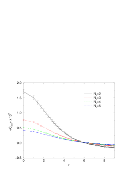
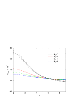
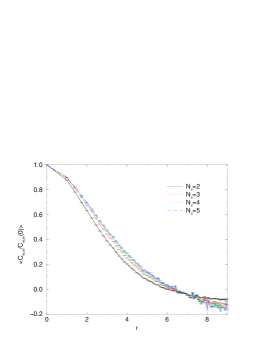
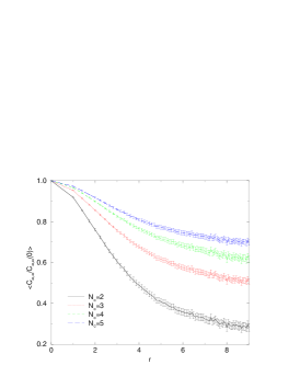
Figure 9: Autocorrelation functions of the pseudoscalar density for the near-zero modes (left column) and the zero modes (right column).

Similarly to eq. (11) we construct correlation functions of the chiral density with the topological charge density obtained after 10 cooling sweeps,

$$C_{\omega,Q}(r)=\frac{1}{V}\int d^{4}x\omega(x)\frac{1}{\Omega_{3}(r)}\int_{|x-y|=r}d^{4}yQ(y).$$ (12)

The results are shown in figure 10 where we show $C_{\omega,Q}(r)$ averaged over all the non-zero modes below the cutoff $\lambda^{2}<0.1$ in the left column and the average over all the zero modes in the right column.

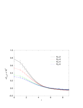
Figure 10: Correlation functions of topological charge density and pseudoscalar density for the near-zero modes (left column) and the zero modes (right column). The topological charge density is taken after 10 cooling sweeps.

The features are very similar to the ones observed in the case of the pseudoscalar density autocorrelation functions. Again the correlators are peaked at small $r$ showing that the pseudoscalar density is large where also the topological charge density is large. Again $C_{\omega,Q}(r=0)$ decreases for increasing $N_{c}$ suggesting that the typical regions with large chirality and topological charge density are less and less localised. However, the typical sizes of regions where the two densities correlate change only weakly with $N_{c}$ for the non-zero modes while the change is again more distinctive for the zero modes. This can be seen again by looking at the corresponding correlators normalised by their value at the origin, cf. the two lower plots in figure 10.

Comparing the mixed correlators $C_{\omega,Q}$ with the autocorrelators $C_{\omega,\omega}$ we observe that the latter are slightly broader. This is just a reflection of the fact that the fermionic eigenmodes are generally less localised compared to the topological charge density due to the different localisation properties of the probing operators. It is also in accordance with the size distributions of objects found in the pseudoscalar and topological charge density, respectively (see section III.4).

All the features observed above are exactly what one would expect from a model of interacting instantons and anti-instantons. The zero modes typically couple to the few narrowest (anti-)instantons which overlap and interact weakly with each other and with other charges, while the non-zero modes couple to the bulk of broader instantons which interact with each other more strongly. The fact that the very small instantons are suppressed for larger $N_{c}$ while the bulk of instantons is only weakly affected by going to larger $N_{c}$ explains the qualitatively different behaviour of the zero modes and the non-zero modes.

For completeness let us now look at the autocorrelation of the topological charge density. Again we define the correlators as in eq. (11) with the pseudoscalar density $\omega(x)$ replaced by the topological charge density $Q(x)$. The resulting correlators are shown in figure 11.

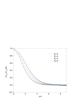
Figure 11: Autocorrelation functions of the topological charge density after 10 cooling sweeps.

The characteristic features are very similar to the ones seen in the autocorrelation functions of the pseudoscalar density of the near-zero modes (cf. left column of figure 9). Again, the peaking of the correlators at small $r$ indicates that the density is concentrated in localised regions. However, it is evident that the apparent localisation of the topological charge is less and less pronounced as we go to larger $N_{c}$. This is reflected both in the values of the correlators at the origin (cf. table 8 in the appendix) as well as in the fall-off of the correlators which becomes slightly weaker for larger $N_{c}$. Again, this is most easily seen by normalising the correlators by their value at the origin, cf. lower plot in figure 11.

III.4 Instanton size distributions

To further corroborate our findings in the previous sections we attempt to generate the size distributions of topological, instanton-like objects from both the topological charge density and the (pseudo-)scalar density of the eigenmodes. In order to do so we identify peaks in the densities and relate the shape of the density distribution around those peaks directly to the instanton radius $\rho$.

To be more precise, we assign a size $\rho$ to each peak $\omega(x_{0})$ in the (pseudo-)scalar density of the eigenmodes by assuming an instanton profile

$$\omega_{I}(x;x_{0})=\pm\frac{2\rho^{2}}{\pi^{2}(\rho^{2}+(x-x_{0})^{2})^{3}}$$ (13)

corresponding to the (pseudo-)scalar density of an eigenmode from a single instanton configuration. We then make the assumption that the low-lying eigenmodes are just linear combinations of such instanton and anti-instanton modes, cf. eq. (3). However, a priori we do not know the weight with which an (anti-)instanton mode contributes to a lifted mode. By forming ratios of the (pseudo-)scalar density at neighbouring points, i.e. by looking at the shape rather than just the peak value of the (pseudo-)scalar density we can cancel out these unknown factors $c_{I}$. Thus using eq. (13) for the peak and its neighbouring points we obtain

$$\rho^{2}=\frac{\sqrt[3]{d}}{1-\sqrt[3]{d}},\quad d=\frac{1}{8}\sum_{\mu=1}^{4}\frac{\omega(x_{0}+\hat{\mu})+\omega(x_{0}-\hat{\mu})}{\omega(x_{0})}.$$ (14)

Similarly, we assume for each peak $Q(x_{0})$ in the topological charge density an instanton profile

$$Q_{I}(x;x_{0})=\frac{6}{\pi^{2}}\frac{\rho^{4}}{(\rho^{2}+(x-x_{0})^{2})^{4}}.$$ (15)

The radius $\rho$ is then calculated from the fall-off of the topological charge density, i.e. from the shape of the instanton profile according to

$$\rho^{2}=\frac{1}{1-\sqrt[4]{d}},\quad d=\frac{1}{8}\sum_{\mu=1}^{4}\frac{Q(x_{0}+\hat{\mu})+Q(x_{0}-\hat{\mu})}{Q(x_{0})}.$$ (16)

To summarise we essentially apply the same procedure for the identification of instanton-like objects and for the calculation of their sizes to both the topological charge density and the (pseudo-)scalar density of the eigenmodes.

Before discussing the results we should point out the limitations and the reliability of such an approach. For both the distributions from the topological charge density and from the (pseudo-)scalar density, the analysis outlined above is limited by the fact that a peak has to be prominent enough in order to stand out of the background fluctuations. This provides a natural cut-off for very broad objects having a flat profile. This constraint, however, is not rigid and therefore puts a limitation on the accuracy of the size distribution for large radii $\rho$, that is, one should exercise caution when considering the tail of the distribution for large $\rho$. On the other hand, due to the finite resolution of the probing operators as discussed in section III.1, there is a lower cut-off for the size of objects which can be seen at all.

Furthermore, a problem which we face by looking at the peaks in the (pseudo-)scalar density of the fermionic modes is the fact that a topological object can cause a prominent peak in several of the eigenmodes, although they might be slightly shifted and distorted. In order to avoid a multiple counting of those peaks we collect all the peaks present in the eigenmodes of a given configuration and impose a minimal distance $r_{\text{min}}$ between any two peaks in order to count as two separate ones. If two or more peaks lie within this minimal radius, all are discarded but the one yielding the smallest radius. While the size distributions from the topological charge density is obviously not much affected by a change in $r_{\text{min}}$, the distributions from the (pseudo-)scalar densities are more sensitive. However, it is interesting to see that a change in $r_{\text{min}}$ almost exclusively affects only the larger objects and not the tail of the distribution at small $\rho$. Another approach is to use the cumulated density of the modes in a given configuration, i.e. to identify the peaks in

$$\omega(x)=\sum_{\lambda}\psi_{\lambda}^{\dagger}(x)\Gamma\psi_{\lambda}(x)\,,$$ (17)

where the sum is over all the eigenmodes below a given cut-off and where $\Gamma=\gamma_{5}$ and $1$ for the pseudoscalar and scalar density, respectively. In this way, we collect the peaks from just one density per configuration and so it is less likely to double count some of the peaks. Moreover, small distortions in the shape of the peaks will average out in the sum over the eigenmodes.

Taking all these considerations into account we are quite confident that the size distributions are reasonably accurate in the range of sizes we are most interested in, that is, in the range $2.0<\rho/a<6.0$.

Figure 12 collects the size distributions obtained from the topological charge densities for the different $N_{c}$. Here we use the topological charge density after 10 cooling sweeps and impose $r_{\text{min}}/a=2.0$.

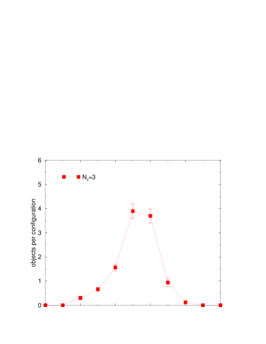
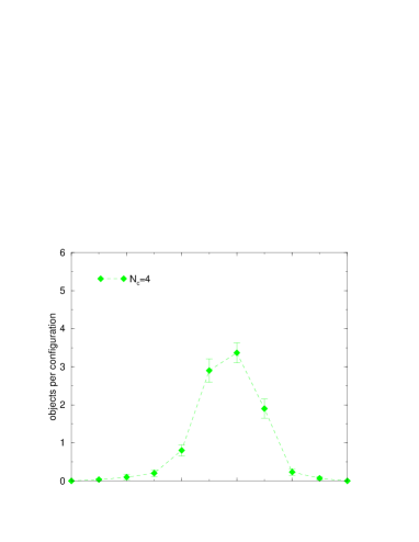
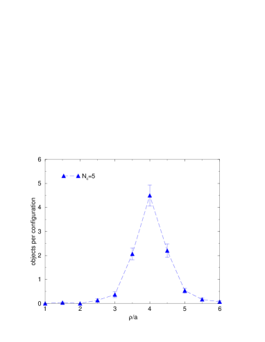
Figure 12: The size distribution of instanton-like objects as seen in the topological charge density after 10 cooling sweeps. The radius is calculated from the shape around the peak value, cf. eq. (16).

There are two important features of the distributions for which a change is evident as we go to larger $N_{c}$. Firstly, the peak of the distribution moves slowly from about $\rho/a\simeq 3.0$ for $N_{c}=2$ to about $\rho/a\simeq 4.0$ for $N_{c}=5$. In physical units this amounts to a change of roughly 0.12 fm in the size of the bulk instantons, i.e. from $\rho\simeq 0.36$ fm to $\rho\simeq 0.48$ fm. It supports our conclusion from section III.3 that the typical size of regions with large topological charge density is slowly growing and thereby causing only a weak broadening of the correlation functions of the near-zero modes, which mainly couple to the bulk of the topological objects.

Secondly, we observe a suppression of small instantons at large $N_{c}$ which is quite dramatic for instantons smaller than $\rho/a\lesssim 3.0$ and still clearly visible for objects with $\rho/a\simeq 3.5$. Again this supports our conclusion from section III.3 where we found that the correlation functions of the topological charge density with the pseudoscalar density of the zero modes broaden considerably for larger $N_{c}$. This is exactly what one would expect if the zero modes couple mainly to only a few rather small objects. On the other hand the near-zero modes are expected to mainly couple to the bulk of instantons not just the smallest ones. One would therefore expect the correlation functions to depend only weakly on $N_{c}$ since the size distribution of the bulk of instantons is only slightly shifted. The correlation functions in section III.3 comply indeed with these expectations.

It is now interesting to look at the size distributions obtained from identifying peaks in the (pseudo-)scalar densities of the near-zero modes and the zero modes. In figure 13 we show the size distributions for the eigenmodes of the different gauge groups. The plots in the left column contain the distributions from the non-zero modes below $\lambda^{2}<0.1$ while the plots in the right column show the distributions from the zero modes. Here we use the cumulated pseudoscalar density, cf. eq. (17). . The sum is taken over all the non-zero modes with $\lambda^{2}<0.1$ or all the zero modes of a given configuration and we impose again $r_{\text{min}}/a=2.0$. It is important to note that these size distributions do not involve any cooling or smearing of the underlying gauge field configurations at all.

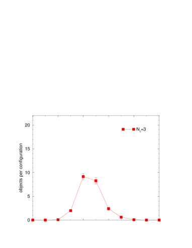
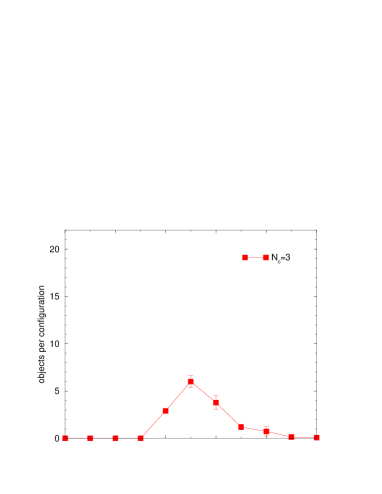
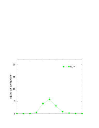
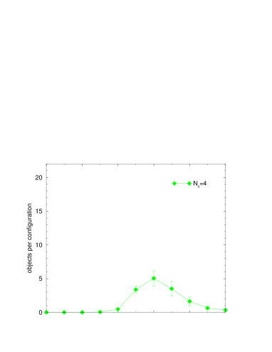
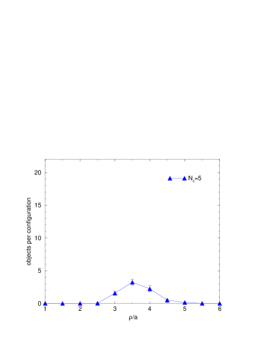
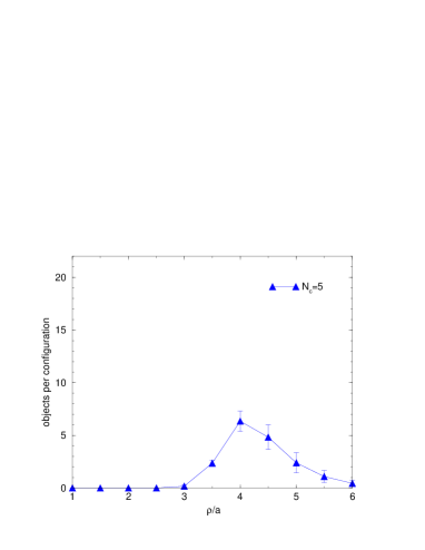
Figure 13: The size distribution of instanton-like objects as seen in the cumulated pseudoscalar density of the near-zero modes with $\lambda^{2}<0.1$ (left column) and the cumulated scalar density of the zero modes (right column). The radius is calculated from the shape around the peak value, cf. eq. (13).

Let us first concentrate on the size distributions calculated from the cumulated pseudoscalar densities of the near-zero modes (plots in the left column). The two main features already observed in the distributions obtained from the topological charge densites are essentially reproduced. Firstly, as we increase $N_{c}$ from 2 to 5 the peak of the distribution moves slowly from about $\rho/a=3.0$ to about $\rho/a=3.5$. So, as we increase $N_{c}$ the regions with pronounced chiral density slowly become more delocalised. Again, this complies with our conclusion from the autocorrelation functions of the chiral densities in section III.3, where we observed that the typical size of local chirality regions in the near-zero modes changes only slightly with increasing $N_{c}$. Secondly, the suppression of small instantons at large $N_{c}$ is again clearly visible. It is most evident for instantons smaller than $\rho/a\lesssim 3.0$ and still apparent for objects with $\rho/a\simeq 3.5$. By contrast, the number of objects with $\rho/a\gtrsim 4.0$ is completely unaffected by an increase in $N_{c}$. In addition to these two features, we also observe that the total number of objects seen in the chiral densities decreases significantly as we go from SU(2) to SU(5) indicating that the chiral densities of the eigenmodes become not only more delocalised but simultaneously smoother for larger $N_{c}$.

The two characteristic features are also present in the size distributions obtained from the cumulated (pseudo-)scalar densities of the zero modes. The peak of the distribution moves from about $\rho/a\simeq 3.0$ for SU(2) to about $\rho/a\simeq 4.0$ for SU(5) and we observe a suppression of objects smaller than $\rho/a\simeq 3.5$ as we increase $N_{c}$. Essentially all instanton-like objects with $\rho/a\lesssim 3.0$ have disappeared by the time we arrive at $N_{c}=5$ or even $N_{c}=4$.

Of course there is a large freedom in how the distributions are extracted from the eigenmodes. So, in addition to the distributions in figure 13 one can also obtain size distributions from the scalar densities of the near-zero modes as well as from the uncumulated scalar and chiral densities of both the near-zero and zeromodes. Moreover, one can look at the distributions for a large range of varying parameters. For example, we may consider the peaks from only the lowest few modes with $\lambda^{2}<0.03$ in each configuration instead of all the modes below our cut-off $\lambda^{2}<0.1$. The results further support our confidence in the distributions so obtained: the shape of the distributions remains exactly the same – it is only the total number of objects that changes. In fact it turns out that the total number of objects seen in the densities differs considerably for the various distributions. This is already clear by comparing for example the distributions in figure 12 with the ones in figure 13. By contrast, the qualitative features, in particular the behaviour at large $N_{c}$, essentially persist in all the distributions we looked at.

To summarise we can confidently say that we observe a shift in the typical sizes of the bulk of instanton-like objects from about 0.36 fm to 0.48 fm as we increase $N_{c}$ from 2 to 5 and a suppression of small instantons with $\rho\lesssim 0.45$ fm at large $N_{c}$.

IV Conclusions

There have been a number of lattice calculations, during this past year, that have addressed long-standing conjectures concerning the role of topology in driving the spontaneous breaking of chiral symmetry. The resurgence of interest in these questions has been largely driven by the recent development of lattice fermion actions, such as overlap fermions, that possess exact topological zero modes and good chiral symmetries at finite lattice spacing.

The main aim of this paper has been to perform an analysis for various SU($N_{c}$) gauge groups in order to address directly an old puzzle that has motivated many of these recent studies: instantons are expected to disappear from the vacuum as $N_{c}\to\infty$ while chiral symmetry breaking is expected to persist.

As a preliminary to addressing this question we needed to determine how well the overlap Dirac operator resolves lattice topology for the moderately coarse lattice spacings, $a$, with which we work. To address this question we compared the fermionic topological charge, $Q_{f}$, obtained from the number of exact zero modes, with the gluonic topological charge, $Q_{g}$, obtained by first cooling the lattice field and then integrating its topological charge density. In SU(2) and SU(3) we found that $Q_{f}$ and $Q_{g}$ frequently disagree with each other; but that any such mismatch becomes rapidly less frequent as we go to larger $N_{c}$. At the same time we found, as observed earlier, that the gauge vacuum rapidly loses all small instantons as $N_{c}$ increases, so that the distinction between physical topology and lattice artifacts becomes unambiguous even for our modest value of $a$. The ‘clean’ character of the large-$N_{c}$ vacuum enabled us to show that in fact the disagreements between $Q_{f}$ and $Q_{g}$ arise because the former does not resolve topological charges which are smaller than about $\rho\simeq 2.5a$ (as calculated after ten cooling sweeps). This demonstrates that $Q_{f}$ is indeed a good measure of lattice topology: it excludes (near-)dislocations but includes all the physical continuum-like topology, at least once $a$ is small enough that the corresponding length scales are distinct.

The agreement between $Q_{f}$, which is calculated directly from the Monte-Carlo generated lattice fields, and $Q_{g}$, which is calculated from the fields only after they have been smoothened, also provides reassurance that the process of cooling does not distort the topological content of the lattice fields in some unexpected way. Indeed we found that the agreement between the fermionic and gluonic measures goes well beyond the global topological properties and extends to the qualitative behaviour of the way the size distribution of the topological charges changes as $N_{c}$ increases. This study confirms that at large $N_{c}$ there are essentially no instantons with $\rho\lesssim 0.45$ fm.

Having established how well the overlap Dirac operator sees topology on our lattice fields we proceeded to perform local chirality analyses of the kind that had been previously performed for SU(3). We found that as $N_{c}$ increases the low-lying eigenmodes rapidly lose their definite chirality properties and our results are consistent with this loss becoming total at $N_{c}=\infty$.

Since the gauge fields lose their smaller instantons as $N_{c}$ increases from $N_{c}=2$ to $N_{c}=5$, it is natural to ask whether this might not be responsible for the change in the local chirality properties of the eigenmodes. However this does not appear to be the case: we found that when we excluded from our SU(3) ensemble any lattice fields with small instantons (the large majority), this did not change the local chirality properties appreciably.

We also calculated the pseudoscalar densities of the low-lying eigenmodes and looked at how these are correlated with themselves and with the topological charge density. All the modes, but the zero-modes most dramatically, become more delocalised as $N_{c}$ increases, consistent with the increasing smoothness of the topological charge density and, indeed, of the eigenmode densities.

A straightforward reading of our results would be that instantons, at least those that are readily identifiable as such, do not survive at large $N_{c}$ and do not drive the chiral symmetry breaking there. Such a conclusion must however be regarded as very preliminary; local chirality provides a limited probe of the properties of the vacuum. We are now in the process of performing what we hope will prove to be a more realistic analysis and one which we hope will provide a more definitive answer to these interesting questions.

Appendix

$f_{V}$ [%]	$N_{c}=2$	3	4	5
1.00	5.18(12)	3.32(05)	2.76(04)	2.54(04)
2.00	8.86(17)	5.90(08)	5.01(07)	4.66(06)
6.25	19.90(28)	14.72(14)	13.00(13)	12.30(12)
12.50	33.09(34)	25.27(17)	22.86(18)	21.76(18)

Table 3: Percentages of the wave function fraction $f_{W}$ as a function of volume fraction $f_{V}$. The first column gives the volume fraction of included lattice sites with largest scalar density while the remaining four give the contribution of these points to the total wave function for different $N_{c}$. All eigenmodes with $\lambda^{2}<0.1$ are included.

$f_{V}$ [%]	$N_{c}=2$	3	4	5
1.00	0.577(33)	0.482(52)	0.394(53)	0.360(56)
2.00	0.539(28)	0.447(40)	0.365(37)	0.333(48)
6.25	0.477(19)	0.383(19)	0.315(23)	0.286(31)
12.50	0.438(15)	0.343(10)	0.286(15)	0.259(24)

Table 4: Weighted average value of the chirality angle $\langle|X|\rangle$, cf. eq. (10), for different $N_{c}$ from all eigenmodes with $\lambda^{2}<0.1$. The first column denotes the volume fraction $f_{V}$ of included points.

$f_{V}$ [%]	$N_{c}=2$	3	4	5
1.00	0.387(25)	0.276(28)	0.192(29)	0.164(29)
2.00	0.348(21)	0.243(21)	0.169(20)	0.144(24)
6.25	0.287(14)	0.189(09)	0.133(12)	0.111(15)
12.50	0.250(10)	0.158(04)	0.113(07)	0.094(11)

Table 5: Weighted average value of the chirality angle $\langle|X|^{2}\rangle$, cf. eq. (10), for different $N_{c}$ from all eigenmodes with $\lambda^{2}<0.1$. The first column denotes the volume fraction $f_{V}$ of included points.

$f_{V}$ [%]	$N_{c}=2$	3	4	5
1.00	0.209(17)	0.110(10)	0.059(11)	0.045(10)
2.00	0.179(14)	0.091(07)	0.048(08)	0.037(07)
6.25	0.134(08)	0.062(02)	0.033(04)	0.024(04)
12.50	0.110(06)	0.047(01)	0.026(02)	0.019(03)

Table 6: Weighted average value of the chirality angle $\langle|X|^{4}\rangle$, cf. eq. (10), for different $N_{c}$ from all eigenmodes with $\lambda^{2}<0.1$. The first column denotes the volume fraction $f_{V}$ of included points.

$f_{V}$ [%]	$N_{c}=2$	3	4	5
1.00	1.61(25)	1.55(34)	1.42(51)	1.32(55)
2.00	1.52(21)	1.46(27)	1.32(38)	1.22(48)
6.25	1.36(15)	1.26(12)	1.12(25)	1.01(33)
12.50	1.24(12)	1.11(07)	0.98(15)	0.87(26)

Table 7: Value of the chirality cumulant $3-\langle|X|^{4}\rangle/\langle|X|^{2}\rangle^{2}$ for different $N_{c}$ from all eigenmodes with $\lambda^{2}<0.1$. The first column denotes the volume fraction $f_{V}$ of included points.

$N_{c}$	$\langle C_{Q,Q}(0)\rangle\cdot 10^{7}$	$\langle C_{\omega,\omega}(0)\rangle\cdot 10^{9}$	$\langle C_{\omega,Q}(0)\rangle\cdot 10^{8}$	$\langle\tilde{C}(0)\rangle$
2	4.27(35)	1.711(79)	0.771(61)	0.29(3)
3	2.34(16)	0.766(23)	0.534(25)	0.40(3)
4	1.34(10)	0.509(14)	0.351(16)	0.43(3)
5	1.30(11)	0.413(10)	0.305(14)	0.42(3)

Table 8: Values of the correlation functions $\langle C_{Q,Q}(0)\rangle,\langle C_{\omega,\omega}(0)\rangle,\langle C_{\omega,Q}(0)\rangle$ at the origin for the near-zero modes. The last column gives the ratio defined by $\tilde{C}(0)=\langle C_{\omega,Q}(0)\rangle/\sqrt{\langle C_{Q,Q}(0)\rangle\langle C_{\omega,\omega}(0)\rangle}$.

$N_{c}$	$\langle C_{\omega,\omega}(0)\rangle\cdot 10^{9}$	$\langle C_{\omega,Q}(0)\rangle\cdot 10^{8}$	$\langle\tilde{C}(0)\rangle$
2	17.19(35)	1.727(163)	0.31(4)
3	4.210(93)	1.117(58)	0.36(3)
4	3.512(66)	0.737(50)	0.34(2)
5	3.174(47)	0.707(53)	0.35(3)

Table 9: Same as table 8 but for the zero modes.