DESY 01-204
                                                                     CPT-2001/P.4272
From enemies to friends: chiral symmetry on the lattice

Abstract

The physics of strong interactions is invariant under the exchange of left-handed and right-handed quarks, at least in the massless limit. This invariance is reflected in the chiral symmetry of quantum chromodynamics. Surprisingly, it has become clear only recently how to implement this important symmetry in lattice formulations of quantum field theories. We will discuss realizations of exact lattice chiral symmetry and give an example of the computation of a physical observable in quantum chromodynamics where chiral symmetry is important. This calculation is performed by relying on finite size scaling methods as predicted by chiral perturbation theory.

1 Introduction

Nature as well as physicists like symmetries. The –somewhat amusing– reason for this is that symmetries can be broken. A very important concept is the spontaneous breakdown of a symmetry: here some symmetry is broken down to a situation with less symmetry when tuning a parameter (e.g. the temperature or the coupling strength) of the theory to a critical value. In the process a non-vanishing vacuum expectation value is developed that breaks the symmetry of the interaction. The process is accompanied by the appearance of so-called Goldstone particles (spinwaves) that are massless. This phenomenon comes under the name of the Goldstone theorem. An example is the spontaneous magnetization: a metal at high temperature is in a symmetric state – the elementary magnets or spins can point in any direction such that the net magnetization vanishes. Decreasing the temperature below some critical value, a spontaneous magnetization occurs, the spins point into a prefered direction and the metal becomes magnetic.

Within the standard model of elementary particle interactions we know two places where such a spontaneous symmetry breaking is supposed to have occurred: in the electroweak sector spontaneous symmetry breaking manifests itself in the Higgs phenomenon with the development of a Higgs field expectation value $\langle\Phi\rangle$, giving mass to the elementary particles, and the appearance of Goldstone particles leading to the W- and Z-bosons.

In our theory of strong interactions, quantum chromodynamics (QCD), it is a chiral symmetry that is assumed to be spontaneously broken. This symmetry allows for an interchange of left handed and right handed quarks while leaving physics invariant – at least when these quarks are massless. In this case a scalar quark-antiquark $q\bar{q}$ condensate is developed and the Goldstone particles are identified with the light pions that are observed in nature.

As stated above the occurrence of spontaneous symmetry breaking is an assumption. The phenomenon is inherently non-perturbative and cannot be addressed with approximative methods like perturbation theory. However, even with numerical simulations it is difficult to test, whether a certain model exhibits spontaneous symmetry breaking (SSB). The reason for this becomes clear when the way to detect SSB is considered. Let us choose a system that has a finite physical volume $V$ as would be required for numerical simulations. Further, we couple the system to an external magnetic field. Spontaneous symmetry breaking is tested in a double limit, where first the volume of the system is sent to infinity and then the external magnetic field is sent to zero. If a non-vanishing magnetization remains, spontaneous symmetry breaking is identified. Obviously, such a procedure is unfeasible within the approach of numerical simulations.

The way out is the use of chiral perturbation theory [1]. In this approach chiral symmetry breaking is taken as an assumption with the consequences of the appearance of non-vanishing field expectation values and Goldstone particles. A special situation arises when the size of the box becomes comparable to or even smaller than the Compton-wavelength of the Goldstone particle. Then the corresponding field can be considered as being uniform and it is possible to set up a systematic expansion that starts in the lowest order with an effective lagrangian of this constant mode and then taking systematically higher order fluctuations into account [2].

2 Example of $\Phi^{4}$-theory

Let us give an example of the Ginsburg-Landau or $\Phi^{4}$ theory with $O(N)$-symmetry in four dimensions. The action of this theory is defined by

$$S=\int d^{4}x\frac{1}{2}\left(\partial_{\mu}\Phi(x)\right)^{2}+\frac{1}{2}m_{0}^{2}\Phi(x)^{2}+\lambda_{0}\Phi(x)^{4}+j^{\alpha}\Phi^{\alpha}(x)$$ (1)

with $\Phi$ a $N$-component vector, $m_{0}$ the bare mass, $\lambda_{0}$ the bare quartic coupling and $j^{\alpha}$ a constant external source in direction $\alpha$ of the group $O(N)$.

Expectation values of observables are computed through the partition function or path integral in finite volume $V=L^{4}$,

$$\langle\Phi\rangle_{j,V}=\int{\cal D}\Phi\Phi e^{-S}\;.$$ (2)

Symmetry breaking is detected via a spontaneous magnetization $\langle\Phi\rangle\neq 0$ in the double limit

$$\langle\Phi\rangle=\lim_{j\rightarrow 0}\lim_{V\rightarrow\infty}\langle\Phi\rangle_{j,V}\;.$$ (3)

Chiral perturbation theory can provide now a prediction for the behaviour of $\langle\Phi\rangle_{j,V}$, i.e. the expectation value in finite volume and at non vanishing external field. In a situation when the external field $j$ and $1/V$ are very small, $\langle\Phi\rangle_{j,V}$ is given in terms of the expectation value of $\langle\Phi\rangle$ at $j=0$ and $V=\infty$:

$$\langle\Phi\rangle_{j,V}=f(u)$$ (4)

where $u$ is a scaling variable

$$u=\langle\Phi\rangle jV$$ (5)

that contains the infinite volume and $j=0$ spontaneous magnetization $\langle\Phi\rangle$.

Let us give for completeness the function $f(u)$:

$$f(u)=\frac{u^{2}\eta(u)}{jV}\;\;\;\mathrm{with}\;\;\;\eta(u)=\frac{1}{u}\frac{I_{2}(u)}{I_{1}(u)}$$ (6)

with $I_{1}$, $I_{2}$ modified Bessel functions. The important point here is that these functions only depend on a single scaling variable $u$ and hence on the quantity of interest, the magnetization $\langle\Phi\rangle$.

In an already quite old work [3] the prediction of chiral perturbation theory, eq. (4), was confronted with numerical data. In this test the data obtained through numerical simulations were described very well by the theoretical formulae of chiral perturbation theory and the method of chiral perturbation theory turned out to be very fruitful, at least in this example of a relatively simple model. The lesson that is to be learnt from this example is that finite size effects can actually be used to determine properties of an infinitely large system. In this sense, the finite volume system can be regarded as a probe of the target theory in infinite volume. This gives an entirely new perspective on finite size effects: instead of being afraid of them, they can be used to determine important physical information.

3 The example of quantum chromodynamics

Chiral perturbation theory as well as the lattice method was developed for quantum chromodynamics in order to deepen our understanding of the strong interactions. Still, until relatively recently, both approaches could not really come together, at least in the region of very small quark masses where chiral symmetry starts to get restored. The reason was that the lattice seemed to be lacking the concept of chiral symmetry and for many years the infamous Nielson-Ninomiya theorem [4] was telling us that it would even be impossible to implement chiral symmetry in a consistent way on a lattice.

The situation only changed a few years ago, when an old work by Ginsparg and Wilson [5] was rediscovered [6]. The Ginsparg-Wilson paper contained actually a clue for answering the problem of chiral fermions on the lattice. The interaction of the fermions is described by some particular operator, the Dirac operator, the details of which should not be discussed here. Now, in the continuum theory this Dirac operator anticommutes with a certain 4-dimensional matrix $\gamma_{5}=\mathrm{diag}(1,1,-1,-1)$. On a lattice with non-vanishing lattice spacing $a$, such an anti-commutation property cannot be demanded. If the anticommutation property is insisted on, the fermion spectrum of the lattice theory does not correspond to the one of the target continuum theory.

The suggestion of Ginsparg and Wilson was to replace the anticommutation condition by a relation (now known as the Ginsparg-Wilson (GW) relation) for a lattice Dirac operator $D$:

$$\gamma_{5}D+D\gamma_{5}=aD\gamma_{5}D\;.$$ (7)

Clearly, in the limit that the lattice spacing vanishes the usual anti-commutation relation of the continuum theory is recovered.

The fact that renders the relation eq. (7) conceptually extremely fruitful is that it implies an exact chiral symmetry on the lattice even if the value of the lattice spacing does not vanish [7]. The notion of a chiral symmetry on the lattice is a conceptual breakthrough and renders the lattice theory in many respects to behave like its continuum counterpart with far reaching consequences.

However, as nice as the theoretical progress that followed the rediscovery of the Ginsparg-Wilson relation was as much of a challenge are realizations of operators $D$ that satisfy the Ginsparg-Wilson relation (see [8, 9, 10] for reviews). Let us give a particular example for such a solution as found by H. Neuberger [11] from the overlap formalism [12], based on the pioneering work of D. Kaplan [13]. To this end, we first consider the standard Wilson Dirac operator on the lattice:

$$D_{\rm w}=\frac{1}{2}\left\{\gamma_{\mu}(\nabla_{\mu}^{*}+\nabla_{\mu})-a\nabla_{\mu}^{*}\nabla_{\mu}\right\}$$ (8)

with $\nabla_{\mu}$, $\nabla_{\mu}^{*}$ the lattice forward, backward derivatives, i.e. nearest neighbour differences, acting on a field $\Phi(x)$

$$\nabla_{\mu}\Phi(x) = \Phi(x+\mu)-\Phi(x)$$

$$\nabla^{*}_{\mu}\Phi(x) = \Phi(x)-\Phi(x+\mu)\;.$$

We then define

$$A=1+s-D_{\rm w}$$ (9)

with $0<s<1$ a tunable parameter. Then Neuberger’s operator $D_{\rm N}$ with mass $m$ is given by

$$D_{\rm N}=\left\{1-\frac{m}{2(1+s)}D_{\rm N}^{(0)}+m\right\}$$ (10)

where

$$D_{\rm N}^{(0)}=(1+s)\left[1-A(A^{\dagger}A)^{-1/2}\right]\;.$$ (11)

What is important here in the definition of Neuberger’s operator is the appearance of the square root of the operator $A^{\dagger}A$. This means that $D_{\rm N}$ connects all points of the lattice with each other. Note, however, that despite this the operator is a local operator in the field theoretical sense [15]. In practice, the operator $A^{\dagger}A$ is represented by a matrix that is, unfortunately, very large. Having a physical volume of size $L^{4}$, the number of sites is $N^{4}=(L/a)^{4}$. As the internal number of degrees of freedom per lattice point is $12$, we end up with $A$ being a $(12N^{4})\otimes(12N^{4})$ complex matrix with $N$ typically in the range $10<N<30$ for present days simulations. Hence we have to construct the square root of a very large matrix. What is worse, to compute relevant physical observables, we don’t need the operator $D_{\rm N}$ itself but its inverse. Such an inverse is constructed by iterative methods like the conjugate gradient algorithm and its relatives [14].

The square root can be constructed by a polynomial expansion, normally based on a Chebyshev approximation, or by rational approximations. Both methods give comparable performances in practice. The convergence of the approximation to the square root is determined by the condition number of the (positive definite) matrix $A^{\dagger}A$. When the matrix $A^{\dagger}A$ is normalized such that the largest eigenvalue is one, the condition number is given by the inverse of the lowest eigenvalue. We show in figure 1 the low-lying eigenvalues of $A^{\dagger}A$ for different values of $\beta$ where the parameter $\beta$ is inversely proportional to the coupling strength of the theory.

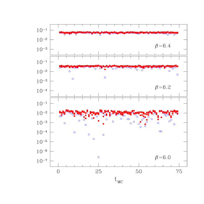
Figure 1: The low-lying end of the eigenvalue spectrum of the matrix $A^{\dagger}A$.

It can clearly be observed that very small eigenvalues can occur resulting in large condition numbers. In such situations the convergence of the approximations chosen can be rather slow and special tricks have to be implemented to accelerate the convergence. The most fruitful improvement is to treat a part of the low-lying end of the spectrum exactly by projecting this part out of the matrix $A^{\dagger}A$ [16, 17]. Further improvements can be implemented, examples of which are discussed in ref. [17].

Despite all these technical improvements it is found that a typical value for the degree of a polynomial is $O(100)$ and a typical value for the number of iterations to compute the inverse of $D_{\mathrm{N}}$ is again $O(100)$. Since in each iteration to compute $D_{\mathrm{N}}^{-1}$ the Chebyshev polynomial has to be evaluated, this means that for a value of a physical observable on a single configuration ten thousand applications of a huge matrix on a vector has to be performed. To compute the expectation value of some observable, this observables has to be averaged over many gluonic configurations. Clearly, this results in a very demanding computational effort and gives rise to a numerical challenge well suited for NIC.

The only thing that helps a lot in this problem is that the matrix $A$ is sparse. Only the diagonal and a few sub-diagonals are actually filled, a fact that finally makes the problem manageable – although, still a very large amount of computer resources are needed to tackle it.

4 The scalar condensate

The existence of an exact lattice chiral symmetry allows the use of finite size effects to test for SSB in QCD as in the case of the $\Phi^{4}$-theory. Using a chiral invariant formulation of lattice QCD, it is possible to reach the region of very small quark masses where it is to be expected that chiral symmetry starts to get restored.

The “magnetization” in the case of quantum chromodynamics is the condensate of a quark-antiquark state $\Sigma=\langle\psi\bar{\psi}\rangle$. The role of the external magnetic field is played by the quark mass $m_{q}$. We have developed a fully parallelized code with all technical improvements implemented. This allowed us to compute the scalar condensate as a function of the quark mass at several volumes. A (standard) caveat here is the fact that all computations are done in the so-called quenched approximation where all internal quark loops are neglected. In QCD there is a peculiarity: the field configurations can have topological properties, characterized by the so-called topological charge which can be measured –unambiguously– through the number of zero modes of the operator $D_{\mathrm{N}}$. In fact, the formulae from quenched chiral perturbation theory are parametrized by the topological charge and it is hence very important to be able to identify the topological charge of the gauge field configurations. Without the special properties of lattice Dirac operators that satisfy the Ginsparg-Wilson relation such an identification would be very difficult.

Let us give the complete theoretical formula from quenched chiral perturbation theory in lowest order:

$$\Sigma_{\nu=\pm 1}(m_{q},V)=\Sigma\;z\;[I_{\nu}(z)K_{\nu}(z)+I_{\nu+1}(z)K_{\nu-1}(z)]+C\cdot m_{q}/a^{2}\;.$$ (12)

The only important thing to notice here is that this relatively involved combination of Bessel functions do, as in the case of the $\Phi^{4}$-theory, only depend on one scaling variable

$$z=\Sigma m_{q}V$$ (13)

that contains the quantity of interest, namely the infinite volume, chiral limit scalar condensate $\Sigma$. The additional term $C\cdot m_{q}/a^{2}$ is a power divergence that comes from the renormalization properties of the theory. We will not discuss this field theoretical aspect here but just notice that this term has to be included in the fit.

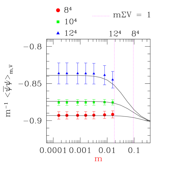
Figure 2: The scalar condensate computed on lattices of various size as a function of the quark mass. The solid lines are 2-parameter ($\Sigma$ and the constant $C$ of eq. (12)) fits according to the prediction of chiral perturbation theory.

In figure 2, we show the result of our numerical computation of the scalar condensate [18] in a fixed topological charge sector $|\nu|=1$ as a function of the quark mass at several volumes. The solid line is a fit to the prediction of chiral perturbation theory, eq.(12). We find that the simulation data are described by this prediction very well. This means that we find evidence for the basic assumption on which the theoretical prediction relies: the appearance of spontaneous chiral symmetry breaking in (quenched) QCD.

We want to remark that this work that has been performed at NIC was the first of this kind. The project consumed 1400 CPU hours on a typical distribution of the lattice on 128 nodes. After this work, a number of other groups repeated such an analysis [21, 22, 23] and it was reassuring to observe that very consistent results were found. In a subsequel work [19, 20] we developed also a quite general method for renormalizing the value of the bare scalar condensate as extracted from the finite size scaling analysis performed here.

5 Conclusion

In this contribution we have demonstrated that by a combination of theoretical ideas, improved numerical methods and the use of powerful supercomputer platforms it is possible to test basic properties of field theories. Of particular interest was the question of whether the phenomenon of spontaneous symmetry breaking does occur in certain field theories important in elementary particle physics. The phenomenon of SSB leads to far reaching consequences in theories like QCD or the scalar sector of the electroweak interactions. In the work performed here, we found strong evidence for the appearance of spontaneous chiral symmetry breaking in quenched lattice QCD. This conclusion is the result of the fact that two theoretical concepts, the lattice approach to quantum field theories and chiral symmetry, met finally – and that enemies became friends.

We are very much indebted to Hartmut Wittig for numerous discussions, suggestions and finally participating in the project at the stage when the non-perturbative renormalization of the scalar condensate was computed. L.L. thanks the INT at the University of Washington for its hospitality and the DOE for partial support during the completion of this work. This work was supported in part by the EU TMR program under contract FMRX-CT98-0169 and the EU HP program under contract HPRN-CT-2000-00145.

References

- [1] S. Weinberg, Physica A96 (1979) 327; J. Gasser and H. Leutwyler, Ann. Phys. (N.Y.) 158 (1984) 142.
-
[2]
J. Gasser and H. Leutwyler,
Phys. Lett. B188 (1987) 477;
H. Neuberger, Phys. Rev. Lett. 60 (1988) 889; Nucl. Phys. B 300 (1988) 180;
F. C. Hansen, Nucl. Phys. B345 (1990) 685; F. C. Hansen and H. Leutwyler, Nucl. Phys. B 350 (1991) 201;
P. Hasenfratz and H. Leutwyler, Nucl. Phys. B 343 (1990) 241. - [3] A. Hasenfratz, K. Jansen, J. Jersák, H.A. Kastrup, C.B. Lang, H. Leutwyler and T. Neuhaus, Nucl. Phys. B356 (1991) 332.
- [4] H. B. Nielsen and M. Ninomiya, Phys.Lett.B105 (1981) 219.
- [5] P.H. Ginsparg and K.G. Wilson, Phys. Rev. D25 (1982) 2649.
- [6] P. Hasenfratz, Nucl. Phys. B (Proc.Suppl.) 63A-C (1998) 53; P. Hasenfratz, V. Laliena and F. Niedermayer, (1998), hep-lat/9801021.
- [7] M. Lüscher, Phys. Lett. B428 (1998) 342, hep-lat/9802011.
- [8] F. Niedermayer, Nucl. Phys. Proc. Suppl. 73 (1999) 105, hep-lat/9810026.
- [9] T. Blum Nucl. Phys. Proc. Suppl. 73 (1999) 167, hep-lat/9810017.
- [10] P. Hernández hep-lat/0110218.
- [11] H. Neuberger, Phys. Lett. B417 (1998) 141, hep-lat/9707022.
- [12] R. Narayanan, H. Neuberger, Nucl.Phys. B412 (1994) 574, hep-lat/9307006.
- [13] D.B. Kaplan, Phys.RLett. B288 (1992) 342.
- [14] W. H. Press, S. A. Teukolsky, W. T. Vetterling and B. P. Flannery, Numerical Recipes, Second Edition, Cambridge University Press, Cambridge, 1992.
- [15] P. Hernández, K. Jansen and M. Lüscher, Nucl. Phys. B552 (1999) 363, hep-lat/9908010.
- [16] R.G. Edwards, U.M. Heller and R. Narayanan, Phys. Rev. D59 (1999) 094510, hep-lat/9811030.
- [17] P. Hernández, K. Jansen and L. Lellouch, hep-lat/0001008.
- [18] P. Hernández, K. Jansen and L. Lellouch, Phys. Lett. B469 (1999) 198, hep-lat/9907022.
- [19] P. Hernández, K. Jansen, L. Lellouch and H. Wittig, JHEP 07 (2001) 18.
- [20] P. Hernández, K. Jansen, L. Lellouch and H. Wittig, (2000), in preparation.
- [21] T. DeGrand, hep-lat/0007046.
- [22] L. Giusti, C. Hoelbling and C. Rebbi, hep-lat/0108007.
- [23] P. Hasenfratz, S. Hauswirth, K. Holland, T. Jorg and F. Niedermayer, hep-lat/0109007.