Study of Confinement Using the
Schrödinger Functional

Abstract

We use a gauge-invariant effective action defined in terms of the lattice Schrödinger functional to investigate vacuum dynamics and confinement in pure lattice gauge theories. After a brief introduction to the method, we report some numerical results.

1 Introduction

To study the vacuum structure of the lattice gauge theories we introduced [1, 2, 3] a gauge invariant effective action, defined by using the lattice Schrödinger functional.

The Schrödinger functional can be expressed as a functional integral [4, 5]

$${\mathcal{Z}}[\mathbf{A}^{(f)},\mathbf{A}^{(i)}]=\int{\mathcal{D}}A_{\mu}\;e^{-\int_{0}^{T}dx_{4}\,\int d^{3}\vec{x}\,{\mathcal{L}}_{YM}(x)}\,,$$ (1)

with the constraints $\mathbf{A}(x_{0}=0)=\mathbf{A}^{(i)}$, $\mathbf{A}(x_{0}=T)=\mathbf{A}^{(f)}$, where $\mathbf{A}(\vec{x})$ are static classical gauge fields. The Schrödinger functional Eq. (1) is invariant under arbitrary static gauge transformations of $\mathbf{A}(\vec{x})$’s fields. The lattice implementation of the Schrödinger functional is discussed in Ref. [6].

Our lattice effective action for the static background field $\mathbf{A}^{\mathrm{ext}}(\vec{x})=\mathbf{A}^{\mathrm{ext}}_{a}(\vec{x})\lambda_{a}/2$ ($\lambda_{a}/2$ generators of the SU(N) algebra) is defined as

$$\Gamma[\mathbf{A}^{\mathrm{ext}}]=-\frac{1}{T}\ln\left\{\frac{{\mathcal{Z}}[U^{\mathrm{ext}}]}{{\mathcal{Z}}[0]}\right\}\,\,,\,\,\,\,\mathcal{Z}[U^{\mathrm{ext}}_{\mu}]=\int_{U_{k}(x)|_{x_{4}=0}=U^{\mathrm{ext}}_{k}(x)}{\mathcal{D}}U\;e^{-S_{W}}\,.$$ (2)

$\mathcal{Z}[U^{\mathrm{ext}}_{\mu}]$ is the lattice Schrödinger functional (invariant, by definition, for lattice gauge transformations of the external links), $U^{\mathrm{ext}}_{\mu}(x)$ is the lattice version of the external continuum gauge field $\mathbf{A}^{\mathrm{ext}}(x)$, and $S_{W}$ is the standard Wilson action. $\mathcal{Z}[0]$ is the lattice Schrödinger functional with $\mathbf{A}^{\mathrm{ext}}=0$ ($U^{\mathrm{ext}}_{\mu}={\mathbf{1}}$).

Our definition of lattice effective action can be extended to gauge systems at finite temperature as

$$\mathcal{Z}_{T}\left[\mathbf{A}^{\text{ext}}\right]=\int_{U_{k}(\beta_{T},\vec{x})=U_{k}(0,\vec{x})=U^{\text{ext}}_{k}(\vec{x})}\mathcal{D}U\,e^{-S_{W}}\,,\,\,\beta_{t}=L_{4}=\frac{1}{aT}\,.$$ (3)

The integrations are over the dynamical links with periodic boundary conditions in the time direction. If we send the physical temperature to zero the thermal functional Eq. (3) reduces to the zero-temperature Schrödinger functional.

2 Abelian Monopoles and Vortices

Monopole or vortex condensation can be detected by means of a disorder parameter $\mu$ defined in terms of the lattice Schrödinger functional $\mathcal{Z}[\mathbf{A}^{\text{ext}}]$ introduced in the previous Section. At zero-temperature

$$\mu=e^{-E_{\text{b.f.}}L_{4}}=\frac{\mathcal{Z}\left[\mathbf{A}^{\text{ext}}\right]}{\mathcal{Z}[0]}\,,$$ (4)

$\mathbf{A}^{\text{ext}}$ is the monopole or vortex static background field. According to the physical interpretation of the effective action Eq. (2) $E_{\text{b.f.}}$ is the energy to create a monopole or a vortex in the quantum vacuum. If there is condensation, then $E_{\text{b.f.}}=0$ and $\mu=1$.

At finite temperature the disorder parameter is defined in terms of the thermal partition function Eq. (3) in presence of the given static background field

$$\mu=e^{-F_{\text{b.f.}}/T_{\text{phys}}}=\frac{\mathcal{Z}_{T}\left[\mathbf{A}^{\text{ext}}\right]}{\mathcal{Z}_{T}[0]}\,,$$ (5)

$F_{\text{b.f.}}$ is now the free energy to create a monopole or a vortex (if there is condensation $F_{\text{b.f.}}=0$ and $\mu=1$).

Our disorder parameter $\mu$ is invariant for time-independent gauge transformations of the external background fields. This implies that we have not to fix the gauge before performing the Abelian projection. Indeed, after choosing the Abelian direction, needed to define the Abelian monopole or vortex fields through the Abelian projection, due to gauge invariance of the Schrödinger functional for transformations of background field, our results do not depend on the selected Abelian direction, which, actually, can be varied by a gauge transformation.

2.1 U(1) monopoles and vortices

In the U(1) l.g.t. we considered a Dirac magnetic monopole background field. In the continuum

$$e\vec{b}({\vec{x}})=\frac{n_{\mathrm{mon}}}{2}\frac{\vec{x}\times\vec{n}}{|\vec{x}|(|\vec{x}|-\vec{x}\cdot\vec{n})}\,,$$ (6)

$\vec{n}$ is the direction of the Dirac string, $e$ is the electric charge and, according to the Dirac quantization condition, $n_{\mathrm{mon}}$ is an integer (magnetic charge = $n_{\mathrm{mon}}/2e$). The lattice implementation of the continuum field Eq. (6) is straightforward. As well we can consider a vortex background field:

$$A^{\text{ext}}_{1,2}=\mp\frac{n_{\text{vort}}}{e}\frac{x_{2,1}}{(x_{1})^{2}+(x_{2})^{2}}\,,\quad A^{\text{ext}}_{3}=0\,.$$ (7)

We can evaluate, by lattice numerical simulation, the energy to create a Dirac monopole or a vortex. It is easier to first evaluate the derivative $E^{\prime}_{\mathrm{mon}}=\partial E_{\mathrm{mon}}/\partial\beta$ ($\beta=1/g$, $g$ is the gauge coupling constant):

$$E^{\prime}_{\text{mon,vort}}=V\left[<U_{\mu\nu}>_{n_{\text{mon,vort}}=0}-<U_{\mu\nu}>_{n_{\text{mon,vort}}\neq 0}\right]\,,$$ (8)

$V$ is the lattice spatial volume. $E_{\text{mon,vort}}$ is then computed by means of a numerical integration in $\beta$. Our numerical results [3] show that Dirac monopoles condense in the confined phase (i.e. for $\beta\lesssim 1.01$) of U(1) lattice gauge theory. While in the case of vortices we do not find a signal of condensation.

Thus, we may conclude that in U(1) lattice theory the strong coupling confined phase is intimately related to magnetic monopole condensation [7].

2.2 SU(2) Abelian monopoles and Abelian vortices

It is well known that SU(2) lattice gauge theory at finite temperature undergoes a transition between confined and deconfined phase. We studied if Abelian monopoles or Abelian vortices condense in the confined phase of SU(2). To this purpose we considered in turn an Abelian monopole and an Abelian vortex background field. We found [3] that both Abelian monopoles and Abelian vortices condense in the confined phase of SU(2).

2.3 SU(3) Abelian monopoles and Abelian vortices

For SU(3) gauge theory the maximal Abelian group is U(1)$\times$U(1), therefore we may introduce two independent types of Abelian monopoles or Abelian vortices associated respectively to the $\lambda_{3}$ and the $\lambda_{8}$ diagonal generator (one can also consider [3] linear combinations of $\lambda_{3}$ and $\lambda_{8}$).

Let us focus on the $\lambda_{8}$ Abelian monopole ($T_{8}$ monopole):

$$U_{1,2}^{\text{ext}}(\vec{x})=\begin{bmatrix}e^{i\theta^{\text{mon}}_{1,2}(\vec{x})}&0&0\\ 0&e^{i\theta^{\text{mon}}_{1,2}(\vec{x})}&0\\ 0&0&e^{-2i\theta^{\text{mon}}_{1,2}(\vec{x})}\end{bmatrix}\,,\quad U^{\text{ext}}_{3}(\vec{x})={\mathbf{1}}\;\,,$$ (9)

with

$$\theta^{\text{mon}}_{1,2}(\vec{x})=\frac{1}{\sqrt{3}}\left[\mp\frac{n_{\text{mon}}}{4}\frac{(x_{2,1}-X_{2,1})}{|\vec{x}_{\text{mon}}|}\frac{1}{|\vec{x}_{\text{mon}}|-(x_{3}-X_{3})}\right]\,.$$ (10)

Analogously, we can define the $T_{3}$ Abelian vortex.

Fig. 1 shows that both $T_{8}$ Abelian monopoles and Abelian vortices condense in the confined phase of SU(3) l.g.t. at finite temperature (simulations have been performed on $32^{3}\times 4$ lattice using the APE100 crate in Bari).

     

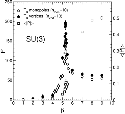
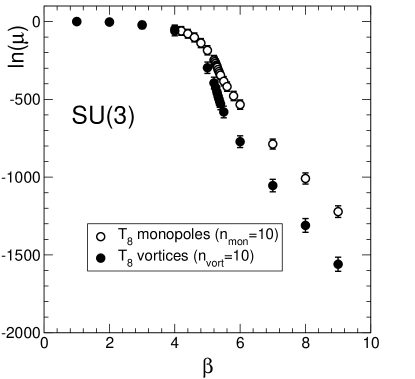
Figure 1: (a) The derivative of the free energy versus $\beta$ for monopoles (open circles) and vortices (full circles). The absolute value of the Polyakov loop is also displayed (open squares). (b) The logarithm of the disorder parameter, Eq. (5), versus $\beta$ for $T_{8}$ monopoles (open circles) and $T_{8}$ vortices (full circles).

2.4 SU(3) Center Vortices

In the case of center vortices the thermal partition function $\mathcal{Z}_{T}[{\mathcal{P}_{\mu\nu}}]$ is defined [8, 9] by multiplying by the center element $\exp(i2\pi/3)$ the set $\mathcal{P}_{\mu\nu}$ of plaquettes $\mathcal{P}_{\mu\nu}(x_{1},x_{2},x_{3},x_{4})$ with $(\mu,\nu)=(4,2)$, $x_{4}=x_{4}^{\star}$, $x_{2}=\frac{L_{s}}{2}$ and $L_{s}^{\text{min}}\leq x_{1,3}\leq L_{s}^{\text{max}}$ , with $L_{s}$ the lattice spatial linear size. By numerical integration of $F^{\prime}_{\text{vort}}$ we can compute $F_{\text{vort}}$ and the disorder parameter $\mu$ (see Eq. (5)). Our numerical results (see Fig. 2) suggest that in the confined phase $F_{\text{vort}}=0$ (in the thermodynamic limit) and center vortices condense.

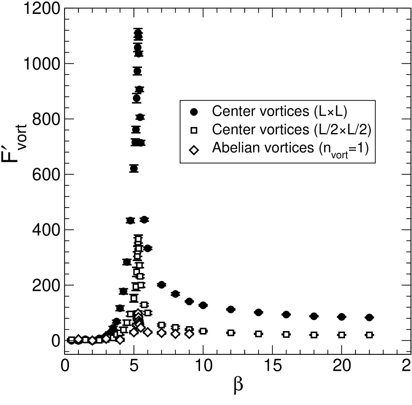
Figure 2: $F^{\prime}_{\text{vort}}$ for center vortices and $T_{8}$ Abelian vortices (vortex charge $n_{\text{vort}}=1$).

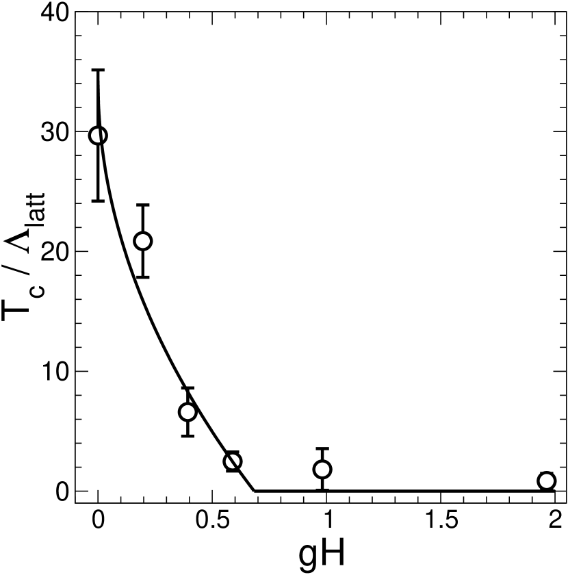
Figure 3: $T_{c}/\Lambda_{\text{latt}}$ versus the applied external field strength $gH$.

3 Constant Abelian Chromomagnetic Field

We want to study the SU(3) gauge system at finite temperature in presence of an external constant Abelian magnetic field

$$\vec{A}^{\mathrm{ext}}_{a}(\vec{x})=\vec{A}^{\mathrm{ext}}(\vec{x})\delta_{a,3}\,,\quad\vec{A}^{\mathrm{ext}}_{k}(\vec{x})=\delta_{k,2}x_{1}H\,.$$ (11)

Spatial links belonging to a given time slice are fixed to

$$U^{\mathrm{ext}}_{1}(\vec{x})=U^{\mathrm{ext}}_{3}(\vec{x})={\mathbf{1}}\,,\quad U^{\mathrm{ext}}_{2}(\vec{x})=\begin{bmatrix}e^{i\frac{gHx_{1}}{2}}&0&0\\ 0&e^{-i\frac{gHx_{1}}{2}}&0\\ 0&0&1\end{bmatrix}\;\,,$$ (12)

that corresponds to the continuum gauge field in Eq. (11). The magnetic field $H$ turns out to be quantized (due to periodic boundary conditions): $a^{2}gH/2=(2\pi)/L_{1})n_{\text{ext}}$ ($n_{\mathrm{ext}}$ integer).

Since the gauge potential in Eq. (11) gives rise to a constant field strength we can consider the density $f[\vec{A}^{\mathrm{ext}}]$ of the free energy functional $F[\vec{A}^{\mathrm{ext}}]$

$$f[\vec{A}^{\mathrm{ext}}]=\frac{1}{V}F[\vec{A}^{\mathrm{ext}}]=-\frac{1}{VL_{t}}\ln\frac{\mathcal{Z_{T}}[\vec{A}^{\mathrm{ext}}]}{{\mathcal{Z_{T}}}[0]}\,,\quad V=L_{s}^{3}\,.$$ (13)

As is well known, the pure gauge system undergoes the deconfinement phase transition by increasing the temperature. The deconfinement temperature in $\Lambda_{\mathrm{latt}}$ units is

$$\frac{T_{c}}{\Lambda_{\mathrm{latt}}}=\frac{1}{L_{t}}\frac{1}{f_{SU(3)}(\beta^{*}(L_{t}))}\,,$$ (14)

where $f_{SU(3)}(\beta)$ is the two-loop asymptotic scaling function and $\beta^{*}(L_{t})$ is the pseudocritical coupling $\beta^{*}(L_{t})$ at a given temporal size $L_{t}$, and can be determined by fitting the peak of $f^{\prime}[\vec{A}^{\mathrm{ext}}]=\partial f[\vec{A}^{\mathrm{ext}}]/\partial\beta$ for the given $L_{t}$.

Following [10] we can perform a linear extrapolation to the continuum of our data for $T_{c}/\Lambda_{\mathrm{latt}}$. We vary the strength of the applied external Abelian chromomagnetic background field in order to analyze a possible dependence of $T_{c}$ on $gH$. We perform numerical simulations on $64^{3}\times L_{t}$ lattices with $n_{\text{ext}}=1,2,3,5,10$. Our numerical results show that the critical temperature decreases by increasing the external Abelian chromomagnetic field. For dimensional reasons one expects that $T_{c}^{2}\,\,\sim\,\,gH\,$ . Indeed we get a satisfying fit to our data with

$$\frac{T_{c}(gH)}{\Lambda_{\text{latt}}}=t+\alpha\sqrt{gH}\,.$$ (15)

From Fig. 3 one can see that there exists a critical field $H_{c}$ such that the deconfinement temperature $T_{c}=0$ for $H>H_{c}$.

References

[1]
P. Cea, L. Cosmai and A. D. Polosa,
Phys. Lett. B 392, 177 (1997).
[2]
P. Cea and L. Cosmai,
Phys. Rev. D 60, 094506 (1999).
[3]
P. Cea and L. Cosmai,
\JHEP0111, 064 (2001).
[4]
D. J. Gross, R. D. Pisarski and L. G. Yaffe,
\RMP53, 43 (1981).
[5]
G. C. Rossi and M. Testa,
Nucl. Phys. B 163, 109 (1980).
[6]
M. Luscher, R. Narayanan, P. Weisz and U. Wolff,
Nucl. Phys. B 384, 168 (1992).
[7]
E. H. Fradkin and L. Susskind,
Phys. Rev. D 17, 2637 (1978).
[8]
T. G. Kovacs and E. T. Tomboulis,
PRL 85, 704 (2000).
[9]
L. Del Debbio, A. Di Giacomo and B. Lucini,
Nucl. Phys. B 594, 287 (2001).
[10]
J. Fingberg, U. Heller and F. Karsch,
Nucl. Phys. B 392, 493 (1993).