DUKE-TH-02-219 Unexpected Results in the Chiral Limit with Staggered Fermions

Abstract

A cluster algorithm is constructed and applied to study the chiral limit of the strongly coupled lattice Schwinger model involving staggered fermions. The algorithm is based on a novel loop representation of the model. Finite size scaling of the chiral susceptibility based on data from lattices of size up to $64\times 64$ indicates the absence of long range correlations at strong couplings. Assuming that there is no phase transition at a weaker coupling, the results imply that all mesons acquire a mass at non-zero lattice spacings. Although this does not violate any known physics, it is surprising since typically one expects a single pion to remain massless at non-zero lattice spacings in the staggered fermion formulation.

1 Motivation

Consider a two dimensional $U(1)$ lattice gauge theory with staggered fermions. This model has been studied extensively on the lattice for over two decades [5, 6, 7, 8, 9, 10, 11]. In the limit when the lattice gauge coupling goes to zero, the model is believed to describe the continuum two flavor Schwinger model; the fermions are confined and the low energy physical particles are mesons. Further, in the chiral limit three massless and one massive pseudo-scalar mesons emerge like in QCD [12]. However, since in two dimensions continuous chiral symmetries remain unbroken, the chiral condensate vanishes in the chiral limit. The actual prediction is

$$\langle\overline{\psi}\psi\rangle\;\sim\;m^{1/3},$$ (1)

as discussed in [13]. This means that the chiral susceptibility $\chi\;=\;\frac{\partial}{\partial m}\langle\overline{\psi}\psi\rangle$ diverges in the chiral limit reflecting the presence of massless excitations. This is consistent with the fact that $M_{\pi}\sim m^{2/3}$, i.e., the pion mass vanishes at $m=0$. If one computes the susceptibility at $m=0$ in a finite box of size $L\times L$, one expects

$$\chi\;\sim\;L,$$ (2)

i.e., it diverges linearly with $L$ [14].

When the lattice gauge coupling is non-zero, lattice artifacts in the staggered fermion formulation break the chiral symmetry of the two flavor Schwinger model explicitly down to a $U(1)$ subgroup. As far as we know, no one has completely analyzed the effects of lattice artifacts on the particle spectrum. Do massless particles remain in the spectrum? The conventional wisdom from higher dimensions is that there should be one massless pion, since the remnant $U(1)$ chiral symmetry is expected to break spontaneously at strong couplings. Of course the Mermin-Wagner theorem forbids the breaking of a continuous symmetry in two dimensions, although non-interacting massless bosons can emerge. On the other hand a $U(1)$ (or equivalently an $O(2)$) symmetry is special. In such a case bosons can interact through topological excitations as discovered by Kosterlitz and Thouless [15]. Thus, the lattice model could either be in a massive or a massless phase depending on the effective couplings of the low energy effective theory describing the bosonic excitations. In the massless phase there are predictions for the behavior of the chiral condensate and the susceptibility based on universality [16]. One expects

$$\langle\overline{\psi}\psi\rangle\;\sim\;m^{\eta/(4-\eta)}.$$ (3)

where $0\leq\eta\leq 0.25$. Again the susceptibility $\chi$ diverges in the chiral limit reflecting the presence of massless excitations. In this case the finite size scaling formula for the susceptibility is given by

$$\chi\;\sim\;L^{2-\eta}.$$ (4)

It is amusing that if we set $\eta=1$ in eqs. (3) and (4) we recover eqs. (1) and (2).

Most results from earlier work on the lattice Schwinger model favor the view point that there is one massless pion at finite lattice spacings. This is based on the observation that the pion mass decreases with the fermion mass like in the continuum Schwinger model. However, on closer examination the lattice model shows deviations, which become larger at stronger couplings as one might expect [8, 9]. On the other hand, no one has ever found scaling relations expected from universality in a massless phase of an $O(2)$ model in two dimensions. In particular no one has been able to confirm relations similar to eqs. (3) or (4). Thus, inspite of the large amount of literature on the subject, questions related to the chiral limit of the lattice Schwinger model with staggered fermions still remain unanswered.

The essential difficulty is the absence of a reliable numerical approach to study interacting fermionic field theories close to the chiral limit. For this reason most previous studies alluded to above, have focused on calculations away from the chiral limit and have used extrapolation techniques to predict the chiral limit. As we will see this can be misleading. In the last few years fermion algorithms based on cluster updates have emerged, which do not suffer from problems that conventional algorithms face near the chiral limit [17]. One can now work directly in the chiral limit using the new approach, a luxury not available with earlier methods. Recently, a fermion cluster algorithm has confirmed the scaling predictions near a Kosterlitz-Thouless transition in a Hubbard type model with unmatched precision [18]. Interestingly, these new ideas can also be applied to study the chiral limit of the lattice Schwinger model at strong couplings [19]. The algorithm is based on a novel loop representation of the model. Although, it may be possible to extend the method to weaker couplings, in this article we concentrate on the strong coupling limit. We focus on the question of whether there are massless excitations at strong couplings by looking for a divergence in the chiral susceptibility as predicted by eq.(4).

2 The Model

The two dimensional $U(1)$ lattice gauge theory with staggered fermions is described by the action

$$S = -\frac{1}{g^{2}}\sum_{x,\mu,\nu,\mu\neq\nu}\mathrm{Re}[U_{\mu}(x)U_{\nu}(x+\hat{\mu})U^{\dagger}_{\mu}(x+\hat{\nu})U^{\dagger}_{\nu}(x)]$$ (5)

$$+\sum_{x,\mu}\;\overline{\psi}_{x}\eta_{\mu}(x)\left(U_{\mu}(x)\psi_{x+\hat{\mu}}-U^{\dagger}_{\mu}(x-\hat{\mu})\psi_{x-\hat{\mu}}\right)$$

$$\hskip 36.135pt+\;m\sum_{x}\overline{\psi}_{x}\psi_{x},$$

where $x\equiv(x_{1},x_{2})$ represents a lattice site on an $L\times L$ lattice, $\mu,\nu=1,2$ represent the two directions and $\hat{\mu},\hat{\nu}$ are the unit vector in the $\mu$ and the $\nu$ direction respectively. The phase factors $\eta_{1}(x)=1$ and $\eta_{2}(x)=(-1)^{x_{1}}$ are the staggered fermion phase factors. The gauge fields $U_{\mu}(x)$ are elements of $U(1)$ phase factors and the fermion fields $\psi(x)$ and $\overline{\psi}(x)$ are Grassmann numbers.

In the strong coupling limit ($g=\infty$) it is possible to integrate over the gauge fields and obtain

$$Z(m) = \;\int[d\psi][d\overline{\psi}]\;\prod_{x}\;\left(1-m\overline{\psi}_{x}\psi_{x}\right)$$ (6)

$$\;\;\;\;\;\;\;\;\;\prod_{x,\mu}\;\left(1+\overline{\psi}_{x}\psi_{x}\overline{\psi}_{x+\mu}\psi_{x+\mu}\right),$$

which can be written as a sum over weights of configurations of monomers and dimers [20]. Each configuration consists of $n_{x}=0,1$ monomers on site $x$ and $b_{x,\mu}=0,1$ dimers on the bond connecting $x$ and $x+\hat{\mu}$. In order for the Grassmann integration to give a non-zero result we need

$$n_{x}+b_{x,1}+b_{x,2}+b_{x-\hat{1},1}+b_{x-\hat{2},2}\;=\;1.$$ (7)

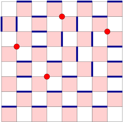
Figure 1: A typical monomer-dimer configuration satisfying eq.(7). The weight of the configuration is $m^{4}$.

Assuming this constraint the partition function can be written as

$$Z(m)\;=\;\sum_{[n,b]}\exp\left[\log(m)\;\sum_{x}\;n_{x}\right]$$ (8)

A typical configuration is shown in figure 1.

When $m=0$ no monomers are allowed and the partition function is given by the number of closely-packed-dimer (CPD) configurations on the lattice. Such configurations are interesting even in condensed matter physics and have played an important role in the study of the 2-d Ising model [21]. The chiral symmetry of staggered fermions is manifest at finite volumes through the fact that the chiral condensate vanishes since it is impossible to find a CPD configuration with just one monomer. The chiral susceptibility on the other hand is non-zero and is a useful observable in the chiral limit. It is equal to the total number of CPD configurations with two monomers, where one of the monomers is constrained to be at a fixed position, divided by the partition function.

3 Loop Representation

It is easy to construct a local Metropolis algorithm for the monomer-dimer model when $m\neq 0$. The algorithm is based on an update which either breaks a dimer into two monomers or vice-versa. This algorithm works reasonably well for $m\geq 0.01$. However, the algorithm fails in the chiral limit since no monomers are allowed when $m=0$. In fact in the chiral limit it is easy to find configurations where simple local updates do not lead to another allowed configuration. Perhaps for this reason, as far as we know, no one has successfully studied the chiral limit.

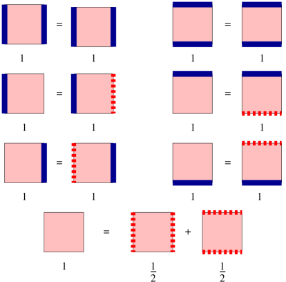
Figure 2: Rules for extending the CPD configurations to include additional bond variables.

To construct an algorithm that is applicable in the chiral limit we extend CPD configurations to configurations of loops made up of bonds which include the original or “filled” dimers (represented here by “solid” bonds) and “empty” dimers (represented by “dashed” bonds) such that the partition function can be expressed as a sum over weights of new loop configurations. Figure 2 shows the rules of one such extension. If we ignore monomers each shaded plaquette of the configuration of Fig. 1 carries one of the seven plaquette configurations given on the left side of equations in Fig. 2. On the other hand, the right side of the equations represent the new configurations and their weights. Figure 3 gives an example of a loop configuration.

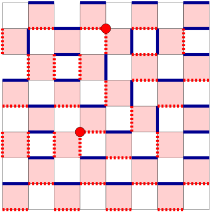
Figure 3: An example of a loop configuration with two monomers.

In the absence of monomers it is easy to check that all constraints are satisfied if each loop is made up of a repeating sequence of filled and empty dimers. This means that there are two allowed configurations associated with each loop. The usefulness of the loop variable is that a dimer system can be updated by “flipping” a loop where filled dimers are emptied and vice versa. The Metropolis acceptance of such a loop flip is found to be reasonable although large loops are not flipped as often as small loops. When monomers are allowed each loop consists of an even number of them. Further, when monomers are present in a loop then it contains a unique pattern of filled and empty dimers and a flip is not allowed. However, close to the chiral limit loops containing monomers are negligible.

The algorithm to measure the susceptibility in the chiral limit is straight forward in the loop representation. Typically, we choose a point at random on the lattice and traverse the loop it is on, starting in the direction of a filled bond. As one goes around the loop, the bonds are flipped and the change in the weight of the configuration is noted. Interestingly, every time a filled bond is emptied one gets a configuration that contributes to the susceptibility. Since its weight relative to the original configuration is known at the time of the flip, it is recorded as a part of the measurement. When the whole loop is flipped one knows the change in the weight of the configuration and a Metropolis accept-reject step can be performed. If the configuration is accepted then one gets a new configuration. Otherwise the loop is flipped back to the original configuration. In any case, the sum over all the weight changes recorded while flipping the filled bonds in the loop divided by one plus the total weight change due to the loop flip is taken as a contribution to the susceptibility during that update. It is possible to show that this algorithm is ergodic.

4 Results

Since the remnant $U(1)$ chiral symmetry of staggered fermions can break spontaneously in higher dimensions, the chiral condensate can approach a constant in the chiral limit. However, in two dimensions a continuous symmetry cannot break and it is almost guaranteed that

$$\langle\overline{\psi}\psi\rangle\;\sim\;m^{\delta}.$$ (9)

with $0<\delta\leq 1$. Comparing with eqs. (1) and (3) we see that $\delta=1/3$ in the continuum two flavor Schwinger model and $\delta\leq 1/15$ is expected from $O(2)$ universality in two dimensions. It is important to remember that the $U(1)$ chiral symmetry of staggered fermions is non-anomalous. Thus, a non-zero expectation value of $\langle\overline{\psi}\psi\rangle$ in the chiral limit would definitely imply a spontaneous breaking of the $U(1)$ symmetry.

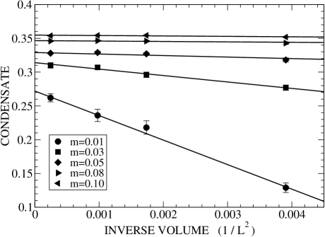
Figure 4: Chiral Condensate as a function of inverse volume at various masses.

Using the local Metropolis algorithm we calculated the chiral condensate for five masses in the region $0.01\leq m\leq 0.1$ for $L=16,24,32$ and $64$. Below $m=0.01$ the algorithm slows down and is not very efficient. Our results are shown in figure 4. The solid lines are linear fits of the data to the finite size scaling formula $\langle\overline{\psi}\psi\rangle=A+B/L^{2}$ at a fixed value of $m$. The constant $A$ then yields the condensate at infinite volume for a fixed mass. Figure 5 shows the condensate as a function of the mass for $L=16$ and for infinite $L$ obtained from fits shown in figure 4. At $L=16$ we see that the condensate goes linearly to zero as expected due to finite volume effects. On the other hand the infinite volume results fit beautifully to a power law of the form $\langle\overline{\psi}\psi\rangle=0.455(6)m^{0.108(5)}$. Since we are in the strong coupling limit it is not surprising that the power does not match the continuum two flavor result of eq. (1). However, it neither matches the predictions of the two dimensional $O(2)$ model based on universality (see eq.(3)).

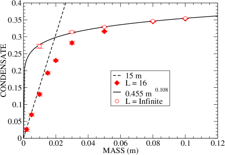
Figure 5: Chiral condensate as a function of mass.

Before attempting to understand the unexpected value of the power it is useful to confirm that the power law behavior is valid all the way to the chiral limit. A power law for the chiral condensate implies that the chiral susceptibility will diverge at $m=0$ in the thermodynamic limit. This divergence typically manifests itself in a finite size scaling of the form

$$\chi=\frac{\partial}{\partial m}\langle\overline{\psi}\psi\rangle\;\sim\;L^{\gamma},$$ (10)

consistent with eqs. (2) and (4). This behavior is difficult to study with conventional algorithms. However, the loop cluster algorithm discussed in the earlier section is designed exactly for this purpose. In figure 6 we plot our results for the chiral susceptibility obtained with the new algorithm at $m=0$ as a function of the lattice size.

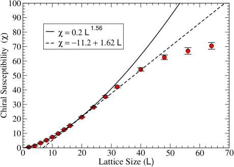
Figure 6: Finite size scaling of the chiral susceptibility.

Notice that for $L=16$ the value of the susceptibility is consistent with $15$, the slope of the condensate at $m=0$ shown in figure 5.

As a function of $L$ the susceptibility behaves differently in different regions. The data is described well by a power law in the region $8\leq L\leq 20$ with $\gamma=1.56$, while a straight line fits the data in the region $20\leq L\leq 40$. For $L>40$ the susceptibility appears to be approaching a constant. If we compare the power law behavior of the susceptibility in the region $8\leq L\leq 20$ with eq. (4) we find that $\eta\sim 0.44$ which is inconsistent with the predictions of $O(2)$ universality in which one would expect $0\leq\eta\leq 0.25$. However, it explains the strange power law behavior of the infinite volume chiral condensate we encountered in figure 5. If we substitute $\eta=0.44$ in eq. (3) we find that $\langle\overline{\psi}\psi\rangle\sim m^{0.12}$, which is quite close to the $L=\infty$ results of figure 5 in the region $0.01\leq m\leq 0.1$. Since the power law behavior of the susceptibility does not extend to larger volumes, it is clear that the power law behavior of the infinite volume chiral condensate shown in figure 5 cannot hold all the way to the chiral limit. In fact the susceptibility at $m=0$ saturates at large volumes. Equivalently, the first derivative of the chiral condensate with respect to the mass at $m=0$ reaches a constant as the volume becomes large. This means the infinite volume chiral condensate will also vanish linearly at $m=0$. Typically, divergence of a susceptibility such as the one defined in eq. (10), is related to the presence of massless particles in the theory. Our results indicate that there are no such particles.

5 Discussion

The results that we have obtained are somewhat surprising. The conventional wisdom is that strong couplings break chiral symmetry at least in three or more dimensions. This suggests that the low energy effective model that describes the $U(1)$ chiral dynamics of the lattice Schwinger model with staggered fermions is most likely in the low temperature (massless) phase at strong couplings. This reasoning appears to be in contradiction with our findings since we do not find the expected divergence described by eq. (4) which in turn implies that there are no massless particles at strong couplings.

Is it possible we have missed something? Of course, we rely heavily on our algorithm. It is rather new and may have weaknesses like long auto-correlation times that we have not yet appreciated. In order to alleviate such fears we have compared our Monte Carlo results with exact calculations of the susceptibility at $m=0$ on small lattices. Table 1 shows this comparison.

Table 1: Chiral Susceptibility: algorithm vs. exact results.

Lattice Size	Exact	Algorithm
$4\times 4$	1.70588235…	1.7059(1)
$6\times 6$	3.33640880…	3.3364(1)
$6\times 8$	4.07961565…	4.0796(2)
$8\times 8$	5.27221660…	5.2722(2)

Clearly, we can reproduce the exact results with great precision at least on small lattices. We have not seen any pathologies in the simulations at larger volumes except for the fact that the fluctuations increase which require us to increase the statistics proportionally. Based on this we are prejudiced to believe in our estimate of the errors within a factor of two or three.

Assuming our results are correct, we find that at strong couplings the lattice model is in the high temperature (massive) phase of the low energy effective model. We know from experience in higher dimensions that chiral symmetry breaking effects become weaker at smaller couplings. This, coupled with the fact that there is no deconfinement transition in two dimensions, suggests that it is unlikely that there is a phase transition to a massless phase at weaker couplings. Our results then imply that there are no massless excitations for all $g\neq 0$ (or equivalently at finite lattice spacings); the non-singlet pseudo-scalar meson (which would be expected to become the Goldstone boson in higher dimensions ) is actually massive at all non-zero couplings. This conclusion may come as a surprise to some, but it does not contradict any known physics as far as we can tell. In particular it does not contradict our expectations that in the zero coupling limit one must recover the continuum two flavor Schwinger model. It is well known that two other non-singlet pseudo-scalar mesons acquire a mass due to lattice artifacts in the staggered fermion formulation. Our data is suggesting that all mesons become massive at non-zero couplings contrary to expectations from higher dimensions where the Goldstone boson will remain massless at finite lattice spacings. In the lattice Schwinger model this boson is still perhaps the lightest. The gauge coupling controls the lattice spacing in the model; typically one uses the mass of the iso-singlet meson to set the lattice spacing. This means that in order to recover the correct continuum limit the singlet and the non-singlet meson masses must become smaller in lattice units as one approaches weaker couplings but their ratio must diverge.

The current work can be extended in many directions. There are results in the large $N_{c}$ and large $d$ limits at strong couplings which show that chiral symmetry is indeed broken [22, 23]. Here we have shown that at $N_{c}=1$ and $d=2$ chiral symmetry remains unbroken and the theory is in the massive phase. It would be interesting to find the value of $N_{c}$ for $d=2$ at which the theory will move into a phase with massless excitations. There is a lot of evidence from lattice simulations and chiral extrapolations that shows lattice QCD with staggered fermions to be in the chirally broken phase. However, as we have seen in the present context, chiral extrapolations can sometimes be misleading. Fortunately, cluster algorithms of the type used here can be developed for any $N_{c}$ and $d$ so that these questions can be answered directly in the chiral limit. One can start with the results presented in [24]. It would be useful to confirm that chiral symmetry is indeed broken at $N_{c}=3$ and $d=4$. On the algorithmic side, it is exciting that we have a new method to explore the chiral limit in certain gauge theories. Loop variables play an important role in this method. Such variables have already been discovered in a limited class of models [25, 26]. Perhaps it is possible to extend them to other interesting models.

References

- [1]
- [2]
- [3]
- [4]
- [5] E. Marinari, G. Parisi, C. Rebbi Nucl. Phys. B190, 734 (1981).
- [6] S.R. Carson and R.D. Kenway (Edinburgh U.), Ann. of Phys. 166, 364 (1986).
- [7] H. Dilger, Nucl. Phys. B434, 321 (1995).
- [8] C. Gutsfeld, H. A. Kastrup, K. Stergio and J. Westphalen Nucl. Phys. (Proc. Suppl.) 63, 266 (1998)
- [9] C. Gutsfeld, H. A. Kastrup and K. Stergio, Nucl. Phys. B560, 431 (1999)
- [10] W. Bietenholz and H. Dilger, Nucl.Phys. B549, 335 (1999).
- [11] Farchioni et al., Phys. Lett. B471, (1999) 58
- [12] C. Gattringer and E. Seiler Annals Phys. 233, 97 (1994).
- [13] S.R. Coleman, Annals Phys. 101, 239 (1976).
- [14] A. Smilga and J.J.M. Verbaarschot, Phys. Rev. D54, 1087 (1996).
- [15] J. M. Kosterlitz and D.J. Thouless, J. Phys. C 6, 1181 (1973).
- [16] J. Zinn-Justin, Quantum Field Theory and Critical Phenomena, 3rd Edition, (Oxford Science Publications), Chapter 32.
- [17] S. Chandrasekharan and U.-J. Wiese, Phys. Rev. Lett 83, 3116 (1999).
- [18] S. Chandrasekharan and J. C. Osborn, cond-mat/0109424.
- [19] S. Chandrasekharan, Nucl. Phys. (Proc.Suppl.) 106, 1025 (2002).
- [20] P. Rossi, U. Wolff, Nucl. Phys. B248, 105, (1984).
- [21] B.M. McCoy and T.T. Wu, The Two-Dimensional Ising Model, Harvard Univ. Press, (1973).
- [22] N. Kawamoto and J. Smit, Nucl. Phys. B192, 100 (1981).
- [23] H. Kluberg-Stern, A. Morel, O. Napoly and B. Petersson, Nucl. Phys. B190, 504 (1981).
- [24] F. Karsch and K.H. Mutter, Nucl. Phys. B313, 541, (1989).
- [25] M. Salmhofer, Nucl. Phys. B362, 641 (1991).
- [26] C. Gattringer, Nucl. Phys. B543, 533 (1999); Nucl.Phys. B559, 539 (1999);