WUB 02-03
Numerical Methods for the QCD Overlap Operator:I. Sign-Function and Error Bounds

Abstract

The numerical and computational aspects of the overlap formalism in lattice quantum chromodynamics are extremely demanding due to a matrix-vector product that involves the sign function of the hermitian Wilson matrix. In this paper we investigate several methods to compute the product of the matrix sign-function with a vector, in particular Lanczos based methods and partial fraction expansion methods. Our goal is two-fold: we give realistic comparisons between known methods together with novel approaches and we present error bounds which allow to guarantee a given accuracy when terminating the Lanczos method and the multishift-CG solver, applied within the partial fraction expansion methods.

, , , , and

1 Introduction

Strongly interacting matter, according to the present standard model of elementary particle physics, is built from quarks interacting by gluons. This hadronic binding problem is highly relativistic: for instance the mass of the proton is 934 MeV while its constituents, the light quarks up and down, carry renormalized masses of about 5 MeV only. The fundamental relativistic gauge theory describing the strong interactions on the level of quarks and gluons is quantum chromodynamics (QCD). Due to asymptotic freedom, the high-momentum sector of QCD can be treated by perturbative methods. However, on the energy scale of the hadronic binding problem, the coupling of QCD becomes large. As a consequence, perturbative methods do not apply to. In a seminal paper of 1974, K. Wilson has proposed to treat QCD numerically on a 4-dimensional space-time lattice. This idea has been brought to life by M. Creutz [1] in the form of a stochastic computer simulation on a 4-dimensional space-time lattice applied to the static quark-antiquark interaction. Today, after two decades of research, simulations by lattice-QCD are considered as the only known way to solve QCD ab initio without recourse to modelling [2].

A serious shortcoming of Wilson’s original discretization of the fermionic sector of QCD [3] is the fact that it violates, at finite lattice spacing $a$, the chiral symmetry of the continuum QCD Lagrangian [4]. Chiral symmetry, which holds at vanishing quark mass, is of vital importance for our understanding of the spectrum of elementary particles. Unfortunately, violation of chiral symmetry through discretization gives rise to a host of lattice artifacts, in particular to additive renormalization of the bare lattice quark mass of the Wilson-Dirac fermion operator,

$$M=I-\kappa D_{W}.$$ (1)

The “hopping term” $D_{W}$ is a non-normal sparse matrix, see eq. (37), coupling nearest neighbours on the 4-dimensional space-time lattice. The associated Green’s function, $G=M^{-1}$, the quark propagator, is a basic building block of both the stochastic simulation and the subsequent computation of hadronic operators. From a numerical point of view, the quantity of interest is $G$ multiplied by a source vector $b$, which can be computed solving the system of equations

$$M\,x=b,$$ (2)

with efficient Krylov-subspace procedures [5, 6, 7]. Such calculations represent the bulk of the computational effort in lattice-QCD simulations.

The recent years have witnessed intensive activity in constructing chiral fermion formulations on the lattice. An intriguing approach has been advanced by Neuberger. His so-called overlap operator [8], defined through

$$D=I-M\cdot(M^{\dagger}M)^{-\frac{1}{2}},$$ (3)

fulfills the Ginsparg-Wilson relation [9] that has been re-discovered by Hasenfratz [10]. It has been shown by Lüscher that this relation implies a novel lattice version of chiral symmetry [11].

The operation of the Green’s function of $D$ on the source vector $b$ can be recast into the equivalent form

$$(r\gamma_{5}+\hbox{\rm\,sign}(Q))x=b\quad(|r|\geq 1),$$ (4)

with $\gamma_{5}$ being defined in eq. (40). The matrix $Q$ is the hermitian form of the Wilson-Dirac matrix, see eq. (39).

The task in solving (4) is two-fold:

1. An outer iteration with the matrix $r\gamma_{5}+\hbox{\rm\,sign}(Q)$ has to be performed. Each step of the outer iteration requires one or two matrix-vector products of the form $\left(r\gamma_{5}+\hbox{\rm\,sign}(Q)\right)\cdot v$.

2. Since $\hbox{\rm\,sign}(Q)$ is not given explicitly, one needs an additional inner iteration for each outer step in order to accurately approximate the product of $\hbox{\rm\,sign}(Q)$ with the generic vector $v$,

   $$s=\hbox{\rm\,sign}(Q)v.$$ (5)

This latter problem has been dealt with in a number of papers, using polynomial approximations [12, 13, 14, 15, 16], Lanczos based methods [17, 18, 19, 20] and partial fraction expansion [21, 22, 23]. For an overview consult Ref. [24]. From these investigations we know that the computational effort in dealing with overlap fermions is at least two orders of magnitude larger than with conventional Wilson fermions due to the repeated application of the sign-function of $Q$ to a vector $v$.

Therefore, it is of particular importance to improve the convergence of the inner iteration process, which is the focus of the present paper: we analyze various known methods and present some novel approaches to iteratively approximate the matrix-vector product with the generic vector $v$ and the hermitian Wilson-Dirac fermion matrix $Q$.

A key issue that we are addressing in this paper is to determine explicit accuracy bounds for each step of the inner iteration. This point is crucial: so far, for error control a fixed order of the given polynomial approximation had to be estimated in advance and/or an additional end-control using the identity $\hbox{\rm\,sign}(Q)^{2}=I$ had to be performed. In practice, this procedure leads to an overhead of at least a factor of two. Furthermore, one might suspect that different stages of the outer iteration require different accuracy of the inner iteration in order to obtain an overall efficient method, see Ref. [25].

This paper is organized as follows: in Section 2 we start by setting up the general Krylov subspace framework that is common to all methods considered in this paper (as well as in the literature known to us). Within this framework, a ‘best-you-can-do’ method can be identified. Though infeasible in practice, this method serves for theoretical comparison purposes, establishing bounds on the maximum performance which cannot be exceeded by any of the considered methods. In Section 3 we shortly describe the Chebyshev approach to approximate (5). This is a numerically feasible method which has already been used repeatedly in QCD computations. Here it will serve as reference for comparison with other approaches, from the practical point of view.

Section 4 discusses various practical methods for approximating (5) with the Lanczos algorithm. We consider known methods as well as new ones and we give a detailed analysis explaining the behavior of the various methods. In addition, within the Lanczos framework, we present a new and cheaply computable convergence criterion through which a given accuracy in the approximation to (5) is guaranteed. In this manner we answer an important question which as yet seems to have remained open.

In Section 5 we turn to the partial fraction expansion (PFE) approach as proposed by Neuberger [21]. Here, (5) is approximated with rational approximations to the sign-function in combination with the multishift-CG algorithm. After discussing two different existing rational approximations used by Neuberger [21] and Edwards et al. [23], we propose a new, best rational approximation based on a result by Zolotarev, see [26]. Our approximation can be computed explicitly, that is there is no need for running the Remez algorithm.

As a result, the number of poles in the rational approximation (and thus the number of shifted systems to be solved concurrently in the shifted CG method) is substantially reduced compared to Ref.  [21] and also Ref. [23].

Moreover, we propose a modification of the multishift-CG method which saves computational work through early termination of converged iterations. Again, we develop a procedure to guarantee a given accuracy. Section 6 presents the results of numerical experiments for realistic computations on a $16^{4}$-lattice performed on the parallel cluster computer ALiCE at Wuppertal University. These results indicate that our new partial fraction expansion approach is the most efficient, at least in the present circumstances where a two-pass strategy for the Lanczos based methods is necessary.

2 Krylov Subspace Framework

The $k$-th Krylov subspace $K_{k}(Q,b)$ of the operator $Q$ with respect to the vector $b$ is the linear space spanned by $b,Qb,Q^{2}b,\ldots,Q^{k-1}b$,

$$K_{k}(Q,b)\equiv\{p_{k-1}(Q)b:p_{k-1}\in\Pi_{k-1}\},$$

with $\Pi_{k-1}$ the space of all polynomials of degree $\leq k-1$.

Krylov subspaces are natural subspaces to approximate vectors of the form $f(Q)b$ with $f$ defined on the spectrum of $Q$, $\mbox{spec}(Q)$, with values in $\mathbb{C}$: If $\mbox{spec}(Q)$ is given as $\mbox{spec}(Q)=\{\lambda_{1},\ldots,\lambda_{n}\}$ and if $p\in\Pi_{n-1}$ interpolates $f$ at the points $\lambda_{1},\ldots,\lambda_{n}$, then $f(Q)b=p_{n-1}(Q)b$, which shows

$$f(Q)b\in K_{n}(Q,b).$$

We can get approximations $x_{k}\in K_{k}(Q,b)$ to $f(Q)b$ by (explicitly or implicitly) computing a polynomial $p_{k-1}\in\Pi_{k-1}$ which approximates $f$ on $\mbox{spec}(Q)$ and setting

$$x_{k}=p_{k-1}(Q)b.$$

Note that $K_{k}(Q,b)\subseteq K_{k+1}(Q,b)$, so building up a basis for the Krylov subspaces can be done in an incremental manner.

In our QCD context we are concerned with situations where $f$ is either the sign-function

$$f(t)=\hbox{\rm\,sign}(t)\equiv\left\{\begin{array}[]{cc}+1&t>0\\ -1&t<0\end{array}\right.$$ (6)

or the inverse modulus

$$f(t)=\frac{1}{|t|}=\frac{1}{\sqrt{t^{2}}}\quad(\hbox{for }t\neq 0).$$ (7)

The following observation is crucial: all methods proposed in the literature on numerical methods for Neuberger fermions known to us – including methods based on rational approximations and all those in the present paper – turn out to be Krylov subspace methods, i.e., they determine (different) approximations $x_{k}\in K_{k}(Q,b)$ for $f(Q)b$ with $f$ from (6) or (7). We therefore have a common Krylov subspace framework to present and analyze these methods.

In this context, when trying to compare different methods, it is certainly interesting to introduce a ‘best you can do method’ – even if such a method is not really feasible from a practical point of view. The ‘best you can do method’ is the following optimal Krylov subspace method: It computes iterates $y_{k}\in K_{k}(Q,b)$ which are best possible in the sense that they have minimal $l_{2}$ distance from $f(Q)b$. This means that $y_{k}$ is the orthogonal projection of $f(Q)b$ onto $K_{k}(Q,b)$ which, given an orthonormal basis $v_{1},\ldots,v_{k}$ of $K_{k}(Q,b)$ can be computed as

$$y_{k}=\sum_{i=1}^{k}v_{i}v_{i}^{\dagger}f(Q)b.$$

Note that in order to get the coefficients $v_{i}^{\dagger}f(Q)b$ we need $f(Q)b$, the quantity we want to compute. So the above optimal method is not computationally feasible a priori. But once we have computed $f(Q)b$ to high accuracy, we can use this ‘best you can do method’ for comparison purposes a posteriori: For any computationally practical Krylov subspace method with iterates $x_{k}\in K_{k}(Q,b)$ one has the inequality

$$\|f(Q)b-x_{k}\|_{2}\geq\|f(Q)b-y_{k}\|_{2},$$

and if the ratio $\|f(Q)b-x_{k}\|_{2}/\|f(Q)b-y_{k}\|_{2}$ is close to $1$, the practical method is a good one. On the other hand, methods for which the ratio $\|f(Q)b-x_{k}\|_{2}/\|f(Q)b-y_{k}\|_{2}$ becomes large are far from being optimal.

The methods that are most often used in computations for QCD applications exploit some polynomial approximation, $s(t)$, for $t^{-1/2}$ and take $p(t)=ts(t^{2})$. Therefore $p$ is an odd polynomial with $p(0)=0$. In general this restriction can have severe consequences. To see this we use the following lemma.

Lemma 1

Define $b^{+}\equiv\frac{1}{2}(I+\hbox{\rm\,sign}(Q))b$ and $b^{-}\equiv\frac{1}{2}(I-\hbox{\rm\,sign}(Q))b$. Let $r_{k}^{+}$ denote the GMRES (see [27]) residual at step $k$ for the equation $Qx=b^{+}$ and similarly, $r_{k}^{-}$ for $Qx=b^{-}$. Then for any polynomial $t\cdot q_{k}(t)$, yielding the approximation $Qq_{k}(Q)b$ we have

$$\|\hbox{\rm\,sign}(Q)b-Qq_{k}(Q)b\|_{2}^{2}\geq\|r_{k+1}^{+}\|_{2}^{2}+\|r_{k+1}^{-}\|_{2}^{2}.$$

[Proof.] We use that $\frac{1}{2}(I+\hbox{\rm\,sign}(Q))$ and $\frac{1}{2}(I-\hbox{\rm\,sign}(Q))$ are the projections onto the two orthogonal invariant subspaces spanned by the eigenvectors corresponding to the positive and negative eigenvalues of $Q$, respectively.

$$\|\hbox{\rm\,sign}(Q)b-Qq_{k}(Q)b\|_{2}^{2} = \|b^{+}-b^{-}-Qq_{k}(Q)(b^{+}+b^{-})\|_{2}^{2}$$

$$= \|b^{+}-Qq_{k}(Q)b^{+}\|_{2}^{2}+\|b^{-}+Qq_{k}(Q)b^{-}\|_{2}^{2}.$$

The proof follows by noting that

$$\|b^{+}-Qq_{k}(Q)b^{+}\|_{2}^{2}\geq\min_{p_{k+1}\in\Pi_{k+1},\\ p_{k+1}^{(0)}=1}\|p_{k+1}(Q)b^{+}\|_{2}^{2}=\|r_{k+1}^{+}\|_{2}^{2}$$

and similar for the system corresponding to the negative part.

To illustrate a possible drawback of a polynomial form with a zero at zero we assume that $Q$ is positive definite. We then have $\hbox{\rm\,sign}(Q)b=b$ and the optimal polynomial is simply given by a polynomial of degree zero. However, from Lemma 1 we see that, if we restrict the approximation to the class of odd polynomials, we need at least a degree equal to the number of iterations required by GMRES for solving $Qx=b$. Which is, in general, much more. In Section 4.4 we show that this restriction on the approximating polynomials is not a severe restriction in QCD applications.

3 The Chebyshev Approach

A common way to get an approximation from a Krylov subspace for a matrix function times a vector is using a suitable polynomial approximation for this function on some set that at least contains the spectrum of the matrix. For the sign-function of $Q$ different polynomial approximations have been proposed on the set $[-b,-a]\cup[a,b]$, if all eigenvalues of $Q$ are contained in this interval. A conceptually very elegant approach is using Gegenbauer polynomials, see [15].

As a reference for the other methods discussed in this paper, we briefly discuss the use of a Chebyshev series and summarize the key points here; for details on the theory see for instance Ref. [28].

Assume for the moment that $f$ is to be approximated on the interval $[-1,1]$. The Chebyshev polynomials $T_{i}(t)\in\Pi_{i}$ are the orthonormal polynomials with respect to the inner product

$$\langle f,g\rangle\equiv\int_{-1}^{1}\frac{1}{\sqrt{1-t^{2}}}f(t)g(t)\hbox{\rm d}t.$$

We thus have

$$\langle T_{i},T_{j}\rangle=\delta_{ij}.$$

Every function $f$ for which $\langle f,f\rangle$ exists can be expanded into its Chebyshev series

$$f=\sum_{i=0}^{\infty}c_{i}T_{i}\enspace\mbox{ with }c_{i}\equiv\langle f,T_{i}\rangle.$$ (8)

Truncating the series at the $k$-th summand gives the polynomial approximation of degree $k$

$$p_{k}=\sum_{i=0}^{k}c_{i}T_{i}$$ (9)

which is ‘best we can do’ in a weighted $L_{2}$-sense, i.e. for all polynomials $q\in\Pi_{k}$ we have

$$\langle p_{k}-f,p_{k}-f\rangle\leq\langle q-f,q-f\rangle.$$

Moreover, $\lim_{i\to\infty}\langle p_{i}-f,p_{i}-f\rangle=0$, which means that we have convergence in a weighted $L_{2}$-sense. If $f$ is continuous, we also have convergence at every point, i.e.

$$\lim_{i\to\infty}p_{i}(t)=f(t)\mbox{ for all }t\in[-1,1].$$

For the approximation of $f$ on a general interval $[\alpha,\beta]$, we use the linear transformation $t\to\frac{1}{\beta-\alpha}(2t-(\beta+\alpha))$ which maps $[\alpha,\beta]$ onto $[-1,1]$. This brings us back to the situation just described.

In a practical numerical computation, the integral defining the coefficient $c_{i}$ in (8) can be approximated by a quadrature rule

$$c_{i}\equiv\frac{2}{k}\sum_{j=1}^{k}f(t_{j})T_{i}(t_{j})\approx\int_{-1}^{1}\frac{1}{\sqrt{1-t^{2}}}f(t)T_{i}(t)\hbox{\rm d}t,$$

with $t_{j}=\cos\left(\pi(j-\frac{1}{2})/k\right)$. Moreover, the approximating polynomial $p_{k}$ from (9) is evaluated by using the numerically stable and efficient Clenshaw-Curtis relation [28, Section 3.2].

For the Dirac overlap operator, truncated Chebyshev series approximations have been introduced by Hernández, Jansen and Lellouch [12, 14]. Here, the polynomial approximations $p_{k}$ from (9) are computed for the function $f(t)=1/\sqrt{t}$ over an interval $[a^{2},b^{2}]$, where $\mbox{spec}(Q)\subseteq[-b,-a]\cup[a,b]$. The approximation to $\hbox{\rm\,sign}(Q)b$ is then obtained as $Q\cdot p_{k}(Q^{2})b$ where $p_{k}(Q^{2})b$ is evaluated using the Clenshaw-Curtis recurrence. We will use this Chebyshev approach as a standard for comparison with the other methods of this paper.

4 Methods Based on the Lanczos Reduction

The polynomials constructed by the methods mentioned in the previous section only depend on the radius of the spectrum, i.e. on $a$ and $b$ with $\mbox{spec}(Q)\subseteq[-b,-a]\cup[a,b]$. In this section and the next one we discuss methods that construct polynomials which use implicitly or explicitly information from the Lanczos reduction. From a practical point of view, this means that they introduce dynamically computed parameters in the construction of the polynomial. Therefore, they are potentially more efficient with respect to the degree of the required polynomial (the number of matrix-vector multiplications) but in general are more expensive to construct (they require inner products and, in general, require more memory). This dichotomy is similar to the one known for iterative methods for linear systems, e.g. [29, Section 2.2].

4.1 Lanczos approximations

The Lanczos method (e.g. [30, 31]) exploits a three-term recurrence for the construction of an orthonormal basis $v_{1}$,$\dots$,$v_{k+1}$ for the subspace $K_{k+1}(A,b)$ as defined in Section 2. This algorithm is given in Alg. 1.

Input: a device to compute $Ax$ and a vector $b$ Output: an orthonormal matrix $V_{k+1}=[v_{1},\dots,v_{k+1}]$ and $T_{k}$ 1. $v_{1}=b/\|b\|_{2}$, $\beta_{0}=0$ for $i=1,2,\ldots,k$ 2. $v=Av_{i}-\beta_{i-1}v_{i-1}$ 3. $\alpha_{i}=v_{i}^{\dagger}v$ 4. $v=v-\alpha_{i}v_{i}$ 5. $\beta_{i}=\|v\|_{2}$ 6. $v_{i+1}=v/\beta_{i}$

Algorithm 1 Lanczos algorithm

The Lanczos algorithm can be expressed in matrix form as

$$AV_{k}=V_{k}T_{k}+\beta_{k}v_{k+1}e_{k}^{\dagger}=V_{k}\underline{T}_{k}$$ (10)

where $T_{k}$ is a $k\times k$ tridiagonal matrix containing the $\alpha_{i}$’s and $\beta_{i}$’s computed in the Lanczos iteration, and $\underline{T}_{k}$ is $T_{k}$ appended with the additional row $\beta_{k}e_{k}^{\dagger}$,

$$T_{k}=\left[\begin{array}[]{ccccc}\alpha_{1}&\beta_{1}\\ \beta_{1}&\alpha_{2}&\ddots\\ &\ddots&\ddots&\ddots\\ &&\ddots&\ddots&\beta_{k-1}\\ &&&\beta_{k-1}&\alpha_{k}\\ \end{array}\right]\enspace\underline{T}_{k}=\left[\begin{array}[]{ccccc}\alpha_{1}&\beta_{1}\\ \beta_{1}&\alpha_{2}&\ddots\\ &\ddots&\ddots&\ddots\\ &&\ddots&\ddots&\beta_{k-1}\\ &&&\beta_{k-1}&\alpha_{k}\\ &&&&\beta_{k}\\ \end{array}\right]\;.$$

We refer to the eigenvalues of $T_{k}$ as the Ritz values (with respect to the search- and test-space $V_{k}$).

A well-known technique, see [32, 33] and the references therein, for the approximation of $f(A)b$ – a matrix function times a vector – is to reduce the problem to a matrix function of the low dimensional matrix $T_{k}$ as in

$$f(A)b\approx V_{k}f(T_{k})V_{k}^{\dagger}b=V_{k}f(T_{k})e_{1}\|b\|_{2}.$$ (11)

The idea of using this Lanczos approximation in (11) for the overlap operator has been considered by several authors. We review the different approaches in this section. Our starting point is the Lanczos algorithm for $Q$ with starting vector $b$, for which the matrix formulation reads

$$QV_{k}=V_{k}T_{k}+\beta_{k}v_{k+1}e_{k}^{\dagger}=V_{k+1}\underline{T}_{k}.$$ (12)

Boriçi [19] applies the Lanczos approximation in (11) to the function $f(t)=(t^{2})^{-1/2}=|t|^{-1}$. This results in

$$\hbox{\rm\,sign}(Q)b=Q|Q|^{-1}\approx QV_{k}{(T_{k}^{2})}^{-1/2}e_{1}\|b\|_{2}=V_{k+1}\underline{T}_{k}{(T_{k}^{2})}^{-1/2}e_{1}\|b\|_{2}.$$ (13)

The first expression is the one originally given in [19]; we have added the second expression to show that the final multiplication with $Q$ can be circumvented by exploiting the vector $v_{k+1}$ in Alg. 1. For more details and a heuristical stopping condition for this method we refer to [19].

A different approach is proposed by van der Vorst [20]. He suggests the following approximation

$$\hbox{\rm\,sign}(Q)b\approx V_{k}\hbox{\rm\,sign}(T_{k})e_{1}\|b\|_{2}.$$ (14)

We note that this approximation is contained in the subspace $K_{k}(Q,b)$ instead of $K_{k+1}(Q,b)$ as for (13). At the end of Section 4.3, we will focus on the difference between both methods.

The errors, as function of $k$, for both methods show large oscillations; see, for instance, Ref. [19, Figure 3] and our discussion in the coming sections. In order to avoid such oscillations, Boriçi has introduced an alternative method based on the Lanczos process for $Q^{2}$ [17]. If we denote the corresponding quantities with hats we obtain

$$Q^{2}\widehat{V}_{k}=\widehat{V}_{k}\widehat{T}_{k}+\widehat{\beta}_{k+1}\widehat{v}_{k+1}e_{k}^{\dagger},$$ (15)

and the resulting approximation is

$$\hbox{sign}(Q)b=Q(Q^{2})^{-1/2}\approx Q\widehat{V}_{k}\widehat{T}_{k}^{-1/2}e_{1}\|b\|_{2}.$$ (16)

Numerical experiments indicate that this method indeed converges smoothly. However, the subspace that contains the approximation $QK_{k}(Q^{2},b)$ is only a subset of the subspace $K_{2k}(Q,b)$, but it requires the same number of matrix vector multiplications (MVs) for its construction (the number of required inner products is less). The question is whether (16) requires many more MVs than (13) and (14) in order to attain a comparable accuracy, see also the discussion following Lemma 1. We return to this question in Section 4.4. In Section 4.3 we consider, for theoretical reasons, another Lanczos approximation based on Lanczos for $Q$, that does have a smoother convergence and we will compare the different methods.

4.2 The idea behind Lanczos approximations

In this section we assume $f$ to be some sufficiently smooth function. The Lanczos approximation (11) implicitly constructs a polynomial $p\in\Pi_{k-1}$ that approximates the function $f$ such that

$$\|f(Q)b-p(Q)b\|_{2}$$ (17)

is small. It is known [34, Theorem 3.3] that this polynomial $p$ interpolates the function $f$ in the Ritz values. To understand the idea behind (11) we consider the more general polynomial $p\in\Pi_{k-1}$ that interpolates $f$ in the (distinct) points $\mu_{i}$, i.e.

$$p(\mu_{i})=f(\mu_{i})\quad\hbox{for }i=1,\dots,k\ ,$$ (18)

and we consider how these $\mu_{i}$ should be chosen such that (17) is small. For this polynomial we have the following bounds for (17):

Lemma 2

For any set of distinct interpolation points $\{\mu_{i}:i=1,\dots,k\}$ and for any function $f\in\mathbb{C}^{k}$, let $p\in\Pi_{k-1}$ satisfy (18) and $q(t)\equiv\prod_{j=1}^{k}(t-\mu_{j})$. Then, if all $\mu_{i}$ and all eigenvalues of $Q$ are contained in the interval $[\alpha,\beta]$ we have

$$\|q(Q)b\|_{2}\inf_{t\in[\alpha,\beta]}\left|\frac{f^{(k)}(t)}{k!}\right|\leq\|f(Q)b-p(Q)b\|_{2}\leq\|q(Q)b\|_{2}\sup_{t\in[\alpha,\beta]}\left|\frac{f^{(k)}(t)}{k!}\right|.$$ (19)

[Proof.] By a standard result on the approximation error of interpolating polynomials, see [35, Thm 2.1.4.1], e.g., there exist values $\xi_{i}\in[\alpha,\beta]$ such that

$$f(\lambda_{i})-p(\lambda_{i})=q(\lambda_{i})\frac{f^{(k)}(\xi_{i})}{k!}.$$

Now, let $b$ be represented as $b=\sum_{i=1}^{n}\gamma_{i}w_{i}$, where the $w_{i}$ are orthogonal and unit length eigenvectors of $Q$ with eigenvalue $\lambda_{i}$. This gives

$$\|f(Q)b-p(Q)b\|_{2}^{2}=\sum_{i=1}^{n}\gamma_{i}^{2}\left(f(\lambda_{i})-p(\lambda_{i})\right)^{2}=\sum_{i=1}^{n}\gamma_{i}^{2}q(\lambda_{i})^{2}\left(\frac{f^{(k)}(\xi_{i})}{k!}\right)^{2}.$$

Bounding this expression results in (19). As discussed in Section 2, finding the polynomial that minimizes (17) is not really feasible. Nevertheless, if $f$ is smooth enough, we can expect nearly optimal results by choosing the $\mu_{i}$’s such that $\|q(Q)b\|_{2}$ is as small as possible. The polynomial that minimizes $\|q(Q)b\|_{2}$ over all monic polynomials in $\Pi_{k}$ is known as the Lanczos polynomial and is equal to $\pi_{k}(t)\equiv\det(tI-T_{k})$, see [36]. Hence, we expect nearly optimal results when the $\mu_{i}$ are equal to the Ritz values. This gives us some justification for the use of (11) and explains the often good experience with this method in practice.

The sign-function has a discontinuity in zero and therefore the result from Lemma 2 cannot be applied. However, we can use that only the function values in the eigenvalues of $T_{k}$ and $Q$ are of importance and we are free to replace the sign-function with some function that has a smooth transition around zero. It can happen in practice that an eigenvalue of $T_{k}$ is close to zero even though the eigenvalues of $Q$ are far from zero. In this case the smoothed sign-function still can have a quite steep transition around zero. In the convergence history of the errors we observe this as a peak in the curve.

In order to achieve smoother convergence for ‘Lanczos on $Q$’ we consider in the next section the use of alternative interpolation points, known as harmonic Ritz values. These are bounded away from zero.

4.3 Smooth convergence with Lanczos on $Q$

The convergence of the methods described by (13) and (14) is rather irregular. In fact, for (13) the error can be infinitely big for a certain $k$ if $T_{k}$ has a very small eigenvalue. For (14) the error never exceeds $2\|b\|$ (because the constructed approximations have the same length as $b$). Therefore the peaks are bounded for this method.

Krylov subspace methods for linear systems that are based on a Galerkin condition, like CG, often show a similar convergence behavior for indefinite problems. In this situation the peaks in the convergence history can cause instabilities in the linear solver, see e.g. [37, 38]. For the Lanczos approximations (13) and (14) of the sign function this poses no serious problem if the case of zero Ritz values is properly handled. It only requires that we skip the result for one iteration. (It can be shown that a Ritz value close to zero in two consecutive iterations implies that this Ritz value is close to an eigenvalue and not a so-called ghost Ritz-value.)

The resulting oscillating behavior led Boriçi to propose his alternative algorithm, which we discussed in Section 4.1. We will propose an alternative for (14) that is still based on (12). The idea is to construct a polynomial $p\in\Pi_{k-1}$ that interpolates $f$ at the harmonic Ritz values instead of the Ritz values. The main reason for this is that the harmonic Ritz values have the property [36] that the smallest harmonic Ritz value (in absolute value) is always outside the interval formed by the largest negative and the smallest positive eigenvalue of $Q$. Therefore, the harmonic Ritz values stay away from the discontinuity in the sign-function.

Our main tool is the following lemma which generalizes a result by Saad [34, Lemma 3.1].

Lemma 3

For all $p\in\Pi_{k-1}$ and all $k$-vectors $z$, we have

$$V_{k}p(T_{k}+ze_{k}^{\dagger})e_{1}\|b\|_{2}=p(A)b.$$ (20)

[Proof.] We show by induction that (20) is correct for all monomials $t^{j}$ with $j<k$. Note that $e_{k}^{\dagger}T_{k}^{j}e_{1}=0$ for $j<k-1$.

$$V_{k}(T_{k}+ze_{k}^{\dagger})e_{1}\|b\|_{2}=V_{k}T_{k}e_{1}\|b\|_{2}=AV_{k}e_{1}\|b\|_{2}-\beta_{k}v_{k+1}e_{k}^{\dagger}e_{1}\|b\|_{2}=Ab$$

Now suppose (20) holds for $t^{i}$ with $i\leq j$ and let $j<k-1$,

$$V_{k}(T_{k}+ze_{k}^{\dagger})^{j+1}e_{1}\|b\|_{2}=V_{k}(T_{k}+ze_{k}^{\dagger})T_{k}^{j}e_{1}\|b\|_{2}=V_{k}T_{k}^{j+1}e_{1}\|b\|_{2},$$

$$V_{k}T_{k}T_{k}^{j}e_{1}\|b\|_{2}=AV_{k}T_{k}^{j}e_{1}\|b\|_{2}+\beta_{k}v_{k+1}e_{k}^{\dagger}T_{k}^{j}e_{1}\|b\|_{2}=A^{j+1}b.$$

This lemma has an interesting corollary which generalizes another result by Saad [34, Theorem 3.3].

Corollary 4

Let $p\in\Pi_{k-1}$ be the unique polynomial that interpolates $f$ in the eigenvalues of $T_{k}+ze_{k}^{\dagger}$. Then we have

$$V_{k}f(T_{k}+ze_{k}^{\dagger})e_{1}\|b\|_{2}=p(A)b.$$

[Proof.] Decompose $f$ in $p+e$ where $p\in\Pi_{k-1}$ is the unique polynomial that interpolates $f$ in the eigenvalues of $T_{k}+ze_{k}^{\dagger}$. We have that $f(T_{k}+ze_{k}^{\dagger})=p(T_{k}+ze_{k}^{\dagger})$. The proof is concluded by using Lemma 3. The harmonic Ritz values are the reciprocals of the Ritz values of $A^{-1}$ with respect to the search- and test-space $AV_{k}$ [36], or, equivalently, the eigenvalues of

$$T_{k}^{-1}\left(T_{k}^{2}+\beta_{k}^{2}e_{k}e_{k}^{\dagger}\right)=T_{k}+ze_{k}^{\dagger}\hbox{ with }z=\beta_{k}^{2}T_{k}^{-1}e_{k}.$$

It is important to realize that the harmonic Ritz values are all distinct (e.g. [36]) and therefore, we have from Corollary 4 the following harmonic Lanczos approximation

$$f(A)b\approx V_{k}f(T_{k}+ze_{k}^{\dagger})e_{1}\|b\|_{2}\hbox{ with }z=\beta_{k}^{2}T_{k}^{-1}e_{k}.$$ (21)

In practical applications the matrix function for the small matrix can be computed using a non-symmetric spectral decomposition (which exists because the harmonic Ritz values are distinct). However, due to the inverse of $T$ this can lead to inaccurate results in case there is a Ritz value close to zero. It is interesting to observe that if $f(t)=t^{-1}$, then the Lanczos approximation is identical to the CG approximation from $V_{k}$ and the harmonic Lanczos approximation is equal to the MINRES approximation. (Note that the usual implementation of MINRES uses a more stable updating procedure than (21).)

Returning to the context of the overlap operator with Lanczos relation (12) the harmonic Lanczos approximation becomes

$$\hbox{sign}(Q)b\approx V_{k}\hbox{sign}(T_{k}+ze_{k}^{\dagger})e_{1}\|b\|_{2}\hbox{ with }z=\beta_{k}^{2}T_{k}^{-1}e_{k}.$$ (22)

We now have three methods to approximate $\hbox{sign}(Q)b$ based on Lanczos for $Q$. We demonstrate their differences for a simple diagonal matrix $Q$. The diagonal of $Q$ contains the elements $-30$,$-29$, $\dots$,$-10$, $1$,$2$,$\dots$,$100$. The vector $b$ has unit-length and all its components are equal. In Figure 1 we plotted the error as a function of $k$. The error of the optimal method is the error of the ‘best you can do method’ from Section 2, computed as $\|(I-V_{k+1}(V_{k+1}^{\dagger}V_{k+1})^{-1}V_{k+1}^{\dagger})\hbox{sign}(Q)b\|$.

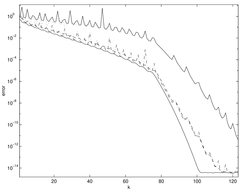
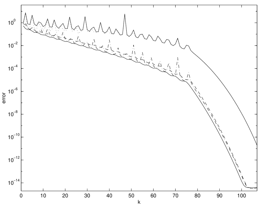
Figure 1: Above: Lanczos without extra orthogonalization, below: Lanczos with extra orthogonalization. optimal (solid lower), Eq. (13) (dotted), Eq. (14) (dash dot), Eq. (22) (dashed), norm of the CG residual (solid top)

From Figure 1 a few features are apparent. In the first place, the loss of orthogonality between the $v_{i}$’s in the Lanczos algorithm due to finite precision arithmetic only delays the convergence, see also [32]. The error for (13) coincides after a while (in norm) with the residual for the CG process. The harmonic Lanczos approximation indeed shows a smoother convergence than the Lanczos approximation but seems in general slightly less accurate. Finally, we note that (14) is in every other step almost optimal and superior to the other approaches. Both (14) and (13) implicitly construct polynomials that interpolate the sign-function on the Ritz values. The approximation in (13) uses the additional degree of freedom for a root in zero. A possible explanation for the better results of (14) in comparison with (13) is that this additional root is a restriction. Further analysis is necessary to understand these phenomena.

4.4 The quality of the polynomials

In this section we compare several ways to construct polynomial approximations to the sign-function by methods from the different classes that we discussed. The methods are the ‘best’ method from Section 2, the Chebyshev approach from Section 3, Lanczos on $Q^{2}$ with (16) and Lanczos on $Q$ with (14). The results for a realistic problem in QCD are given in Figure 2. The lattice is $16^{4}$, $\kappa=0.208$ and $\beta=6$.

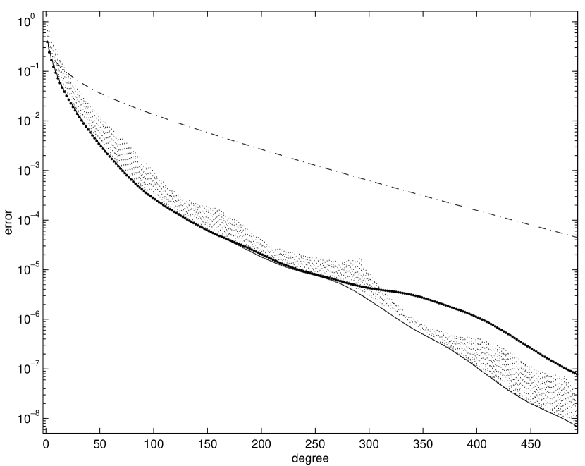
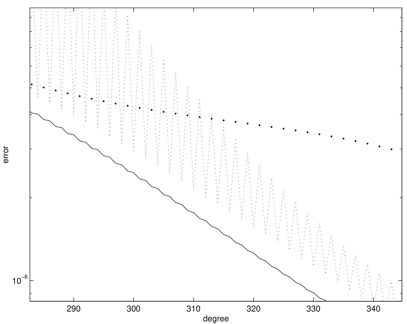
Figure 2: The error as a function of the polynomial degree: optimal (solid), Chebyshev method (-.), Eq. (4.7) (dots), Eq. (4.5) (dotted). The second diagram shows a detail of the first one.

All methods considered are not too far away from the ‘best you can do’ method. It thus appears that for realistic QCD matrices, $Q$, it is not a real drawback to restrict the approximation to the class of odd polynomials (i.e. to the space $QK_{k/2}(Q^{2},b)$), as might have been anticipated from the discussion in Section 2. Therefore, we consider in the remainder of this paper ‘Lanczos on $Q^{2}$’ with (16) as an efficient method within the class of Lanczos approximations.

4.5 Error estimation

An important question is when to terminate Alg. 1 such that the approximation (16) is within a distance $\epsilon$ to the exact vector $\hbox{\rm\,sign}(Q)\cdot b$. In [17] it is proposed to use the norm of the residual of the related CG process as an upper bound for the error in $2$-norm. The norm of this residual can be computed at little additional cost in Alg. 1, see [17] for details. Note that no theoretical justification for this stopping criterion was given in [17]. In this section we will prove that the norm of the CG residual is always larger than the error for (16). This result is formulated in Theorem 6.

For the proof we will use the following integral representation of the inverse square root, see, e.g., [19]:

$$A^{-1/2}=\frac{2}{\pi}\int_{t=0}^{\infty}(A+t^{2}I)^{-1}\hbox{\rm d}t.$$ (23)

Furthermore, we will exploit the following convenient property of the conjugate gradient method applied to a shifted system.

Lemma 5

Let $r_{k}$ denote the CG residual for $k$ steps CG when solving $Ax=b$ and, similarly, $r_{k}^{\tau}$ for solving $(A+\tau I)x=b$, both methods starting with the initial iterate zero. Then

$$r_{k}^{\tau}=\phi_{k}^{\tau}r_{k}$$

with

$$\phi_{k}^{\tau}\equiv\prod_{j=1}^{k}\frac{\theta_{j,k}}{\theta_{j,k}+\tau},$$

where $\theta_{j,k}$ denotes the $j$-th eigenvalue of $T_{k}$.

[Proof.] From e.g. [36] we have the following polynomial characterizations for the residuals

$$\begin{array}[]{ll}r_{k}=\pi_{k}(A)b/\pi_{k}(0),&\pi_{k}(t)\equiv\det(tI-T_{k})\\ r_{k}^{\tau}=\pi_{k}^{\tau}(A+\tau I)b/\pi_{k}^{\tau}(0),&\pi_{k}^{\tau}(t)\equiv\det(tI-(T_{k}+\tau I)).\\ \end{array}$$

Hence,

$$r_{k}^{\tau}=\pi_{k}^{\tau}(A+\tau I)b/\pi_{k}^{\tau}(0)=\phi_{k}^{\tau}\pi_{k}(A)b/\pi_{k}(0)=\phi_{k}^{\tau}r_{k}.$$

We are now in a position to formulate the main theorem in this section.

Theorem 6

Let $\det(Q)\neq 0$. Then

$$\|\hbox{\rm sign}(Q)b-Q\widehat{V}_{k}\widehat{T}_{k}^{-1/2}e_{1}\|_{2}\leq\|r_{k}\|_{2}\leq 2\kappa\left(\frac{\kappa-1}{\kappa+1}\right)^{k}\cdot\|b\|_{2},$$ (24)

where $\kappa\equiv\|Q\|_{2}\|Q^{-1}\|_{2}$ and $r_{k}$ is the residual in the $k$-th step of the CG method applied to the system $Q^{2}x=b$ (with initial residual $b$, i.e. initial guess $0$).

[Proof.] The expression $\hbox{\rm sign}(Q)b-Q\widehat{V}_{k}\widehat{T}_{k}^{-1/2}e_{1}$ can be rewritten with (23) as

$$\frac{2}{\pi}\int_{0}^{\infty}Q(t^{2}I+Q^{2})^{-1}b-Q\widehat{V}_{k}(t^{2}I+\widehat{T}_{k})^{-1}\widehat{V}_{k}^{\dagger}b\ \hbox{\rm d}t=$$

$$\frac{2}{\pi}\int_{0}^{\infty}Q(t^{2}I+Q^{2})^{-1}(t^{2}I+Q^{2})\left((t^{2}I+Q^{2})^{-1}-\widehat{V}_{k}(t^{2}I+\widehat{T}_{k})^{-1}\widehat{V}_{k}^{\dagger}\right)b\ \hbox{\rm d}t=$$

$$\frac{2}{\pi}\int_{0}^{\infty}Q(t^{2}I+Q^{2})^{-1}r^{t^{2}}_{k}\ \hbox{\rm d}t,$$

where $r^{t^{2}}_{k}\equiv b-(Q^{2}+t^{2}I)\widehat{V}_{k}(\widehat{T}_{k}+t^{2}I)^{-1}e_{1}$. With Lemma 5 this can be expressed as

$$\frac{2}{\pi}\int_{0}^{\infty}Q(t^{2}I+Q^{2})^{-1}\phi_{k}^{t^{2}}r_{k}\ \hbox{\rm d}t=Xr_{k}\ \hbox{, with}\ X\equiv\frac{2}{\pi}\int_{0}^{\infty}Q(t^{2}I+Q^{2})^{-1}\phi_{k}^{t^{2}}\ \hbox{\rm d}t.$$ (25)

Then the first bound in (24) follows by bounding the eigenvalues of the operator $X$ in (25). To this purpose, note that the eigenvalues of $X$ are given as

$$\frac{2}{\pi}\int_{0}^{\infty}\lambda_{i}(t^{2}+\lambda_{i}^{2})^{-1}\phi_{k}^{t^{2}}\ \hbox{\rm d}t$$ (26)

with $\lambda_{i}$ the eigenvalues of $Q$. For $\lambda_{i}$ fixed, the integrand in (26) has constant sign. Since $0\leq\phi_{k}^{t^{2}}\leq 1$ we therefore get

$$\left|\frac{2}{\pi}\int_{0}^{\infty}\lambda_{i}(t^{2}+\lambda_{i}^{2})^{-1}\phi_{k}^{t^{2}}\ \hbox{\rm d}t\right|\;\leq\;\left|\frac{2}{\pi}\int_{0}^{\infty}\lambda_{i}(t^{2}+\lambda_{i}^{2})^{-1}\ \hbox{\rm d}t\right|\;=\;1.$$

This proves $\|X\|_{2}\leq 1$ and thus $\|Xr_{k}\|_{2}\leq\|r_{k}\|_{2}$.

The a priori upper bound follows directly from a priori error estimates for CG, as in Theorem 3.1.1 in [29].

The question is how tight the lower bound in (24) may be. After one step of Alg. 1, i.e. for $k=1$, where we have a simple expression for $\phi_{1}^{t^{2}}$, we can explicitly integrate (26). As a result we then see that the residual is overestimated by at most a factor $1+\frac{\lambda}{\sqrt{T_{1}}}$, in the direction of the eigenvector corresponding to $\lambda$. Hence, we are at most a factor $1+\kappa(Q)$ off and at least a factor $1+\kappa(Q)^{-1}$.

When a precision $\epsilon$ is required, the process can be safely terminated as soon as $\|r_{k}\|_{2}\leq\epsilon$.

4.6 Practical implementations

In practice it is not feasible to store all $k$ vectors $\widehat{v}_{i}$ for the evaluation of (16). This problem can be circumvented by executing Alg. 1 twice [19, 17]. In the first step the tridiagonal matrix $\widehat{T}_{k}$ is constructed after which the vector $\widehat{T}_{k}^{-1/2}e_{1}\|b\|_{2}$ is computed. In the second run of Alg. 1 the $\widehat{v}_{i}$’s are combined to compute $\widehat{V}_{k}\widehat{T}_{k}^{-1/2}e_{1}\|b\|_{2}$. This doubles the number of MVs but, as remarked by Neuberger [21], this method can be still competitive because of a potentially better exploitation of the computer memory hierarchy (e.g., cache effects).

Another issue is the computation of $\widehat{T}_{k}^{-1/2}e_{1}\|b\|_{2}$. Our own numerical experiments show that a computation with a full spectral decomposition, as in [17, Algorithm 2], is too CPU-time consuming. Instead it seems natural to exploit the special tridiagonal structure of $\widehat{T}_{k}$ in a similar way as done for the exponential function in [34], for example. In our numerical experiments we computed $\widehat{T}_{k}^{-1/2}e_{1}\|b\|_{2}$ using a rational approximation expanded as the sum over poles (called a partial fraction expansion, PFE)

$$\widehat{T}_{k}^{-1/2}\approx\sum_{i=1}^{m}\omega_{i}(\widehat{T}_{k}+\tau_{i}I)^{-1}.$$

A discussion of the choice of suitable coefficients $\tau_{i}$ and $\omega_{i}$ can be found in Section 5.2. We are now required to solve $m$ tridiagonal linear systems $(\widehat{T}_{k}+\tau_{i}I)z=e_{1}\|b\|_{2}$ and this can be done efficiently with the LAPACK function DPTSV. This results in $O(km)$ flops which can be much less than the $O(k^{2})$ flops that are needed for the computation of a full spectral decomposition. In the remainder of this paper we will refer to this implementation of (16) as Lanczos/PFE.

5 The PFE/CG Method

The Lanczos approximations in the previous section require two passes of the Lanczos method to limit memory requirements. This doubles the number of matrix-vector multiplications. An elegant idea for working with only a fixed number of vectors without requiring two passes was proposed, in the context of QCD, by Neuberger [21]. Suppose $r(t)$ is a rational function approximating the sign-function in the interval $[-b,-a]\cup[a,b]$ that contains the eigenvalues of $Q$. Let $r(t)$ be represented by the following partial fraction expansion

$$\hbox{\rm\,sign}(t)\approx r(t)=\sum_{i=1}^{m}\omega_{i}\frac{t}{t^{2}+\tau_{i}},$$ (27)

then

$$\hbox{\rm\,sign}(Q)b\approx x^{\mbox{pfe}}\equiv r(Q)b=\sum_{i=1}^{m}\omega_{i}\frac{Q}{Q^{2}+\tau_{i}I}b.$$ (28)

The idea is now to solve the $m$ linear systems in (28) with a multi-shift Conjugate Gradient method [39, 40]. The philosophy behind the multi-shift CG method is the following Lanczos relation for shifted matrices

$$(Q^{2}+\tau_{i}I)\widehat{V}_{k}=\widehat{V}_{k}(\widehat{T}_{k}+\tau_{i}I)+\widehat{\beta}_{k}\widehat{v}_{k+1}e_{k}^{\dagger}.$$ (29)

Hence, the orthonormal basis has to be constructed only once for the various shifts and after $k$ steps Lanczos we can construct $m$ approximate solutions and the corresponding residuals as

$$x_{k}^{i}\equiv\widehat{V}_{k}(\widehat{T}_{k}+\tau_{i}I)^{-1}e_{1}\|b\|_{2}\hbox{ and }r_{k}^{i}\equiv b-(Q^{2}+\tau_{i}I)x_{k}^{i}.$$

Similar in spirit to other Krylov subspace methods for shifted linear systems ([39, 41, 42, 40], e.g.) the multi-shift CG method computes these vectors in an efficient way. The final approximation to $\hbox{\rm\,sign}(Q)b$ now reads

$$\hbox{\rm\,sign}(Q)b\approx x^{\mbox{pfe}}\approx x_{k}\equiv\sum_{i=1}^{m}\omega_{i}Qx_{k}^{i}.$$ (30)

We refer to this method as PFE/CG (of course, in a practical implementation the solutions of the $m$ different systems are not stored but are immediately combined to save memory). We are again in the Krylov subspace framework described in Section 2, since $x^{\mbox{pfe}}$ is from the Krylov subspace $K_{l}(Q,b)$ with $l=2k+1$, $k$ being the maximum number of iterations in multi-shift CG. Note also that this method is, for the same shifts and poles, mathematically equivalent to the Lanczos/PFE method from Section 4.6.

5.1 Error estimation

We need a criterion for the termination of the multi-shift CG method such that $x_{k}$ in (30) is close enough to $\hbox{\rm\,sign}(Q)b$, or $\|\hbox{sign}(Q)b-x_{k}\|\leq\epsilon$. The error in the PFE/CG method consists of two parts. First, we demand the following accuracy of the rational function (this can be cheaply monitored in its construction)

$$|\hbox{\rm\,sign}(t)-r(t)|\leq\epsilon/2\hbox{ for }t\in\mbox{spec}(Q)\subset[-b,-a]\cup[a,b].$$ (31)

This gives

$$\|\hbox{\rm\,sign}(Q)b-x^{\mbox{pfe}}\|_{2}\leq\epsilon/2.$$

Furthermore, we require that

$$\|x^{\mbox{pfe}}-x_{k}\|_{2}\leq\epsilon/2.$$

Our termination condition consists of checking if this condition is fulfilled. We use the following theorem for this which is similar in spirit to Theorem 6.

Theorem 7

Let the rational approximation satisfy (31) and $\omega_{i}\geq 0$ for $i\in\{1,\dots,m\}$ and $0<\tau_{1}\leq\tau_{2}\leq\dots\leq\tau_{m}$, then

$$\|x^{\mbox{\rm pfe}}-x_{k}\|_{2}\leq(1+\epsilon/2)\|r_{k}^{1}\|_{2}.$$

[Proof.]

$$x^{\mbox{pfe}}-x_{k}=\sum_{i=1}^{m}\omega_{i}Q\left(\frac{I}{Q^{2}+\tau_{i}I}b-x_{k}^{i}\right)=\sum_{i=1}^{m}\omega_{i}\frac{Q}{Q^{2}+\tau_{i}I}r_{k}^{i}$$

$$=\sum_{i=1}^{m}\omega_{i}\frac{Q}{Q^{2}+\tau_{i}I}\phi_{k}^{(\tau_{i}-\tau_{1})}r_{k}^{1}=Xr_{k}^{1}\hbox{ with }X\equiv\sum_{i=1}^{m}\omega_{i}\frac{Q}{Q^{2}+\tau_{i}I}\phi_{k}^{(\tau_{i}-\tau_{1})}$$

Here, we have used Lemma 5. The proof follows by noting that the eigenvalues of $X$ are of the form $\sum_{i=1}^{m}\omega_{i}\frac{t}{t^{2}+\tau_{i}}\phi_{k}^{(\tau_{i}-\tau_{1})},\;t\in\mbox{spec}(Q)$ and this expression is bounded in absolute value by $|r(t)|$. From (31) we find that $|r(t)|\leq 1+\epsilon/2$ for $t\in\mbox{spec}(Q)$. So, we can terminate the multi-shift CG method when the residual of the first system satisfies

$$\|r_{k}^{1}\|_{2}\leq\frac{\epsilon}{2+\epsilon}.$$ (32)

Then the error of $x_{k}$ is bounded as $\|x_{k}-\hbox{sign}(Q)b\|_{2}\leq\epsilon$.

5.2 The choice of the rational approximation

For the PFE/CG method the cost of computing $\hbox{\rm\,sign}(Q)b$ is basically the cost of one run of CG plus some additional cost for updating of the $m-1$ additional systems. This puts emphasis on the efficiency of the used rational approximation. Let us first make our terminology precise: We consider a given function $f$ which is defined on a set $D$ and we assume that we have a space $S$ of approximating functions, all defined on $D$. Then we call $g\in S$ a best approximation for $f$ on $D$ from $S$, if $g$ minimizes the quantity

$$\sup_{t\in D}|f(t)-h(t)|$$

among all functions $h$ from $S$. In our context, $S$ will be a space $R_{i,j}$ of rational functions $r(t)=p(t)/q(t)$ with $p\in\Pi_{i}$ and $q\in\Pi_{j}$.

In his original proposition, Neuberger [21] uses the following rational approximation from $R_{2m-1,2m}$

$$r(t)=\frac{(t+1)^{2m}-(t-1)^{2m}}{(t+1)^{2m}+(t-1)^{2m}},$$

which can be written in the form of (27) with

$$\omega_{i}=\frac{1}{m}\cos^{-2}\left(\frac{\pi}{2m}(i-\frac{1}{2})\right),\quad\tau_{i}=\tan^{2}\left(\frac{\pi}{2m}(i-\frac{1}{2})\right).$$

It can be easily checked that this approximation is exact for $|t|=1$ and that the error for $|t|\geq 1$ is increasing for increasing $|t|$. From this and $r(t)=r(t^{-1})$ it follows that this rational function approximates $\hbox{sign}(t)$ well on sets $D$ of the form $[-1/c,-c]\cup[c,1/c]$ for some specific value $c\in(0,1]$ (independent of $m$). Therefore, it is common practice to map the interval $[-b,-a]\cup[a,b]$ to a range of the form $[-1/c,-c]\cup[c,1/c]$ by scaling with a factor $(ab)^{-1/2}$, yielding $c=\sqrt{b/a}$.

Another consequence is that the error is maximal for $t=\sqrt{\kappa}$ (see also [23]). Using this it follows that for a precision of $\epsilon/2$ in this scaled interval we need $m$ poles where $m$ is some integer with

$$m\geq\frac{1}{2}\log\left(\frac{\epsilon}{4-\epsilon}\right)\left/\log\left(\frac{\sqrt{b/a}-1}{\sqrt{b/a}+1}\right)\right..$$ (33)

From (33) it appears that the number of required poles can be quite large. The function $r(t)$ is not a best approximation in the sense defined before, see Proposition 8 below.

A different idea is to construct an approximation of the form $\hbox{\rm\,sign}(t)\approx ts(t^{2})$ where

$$t^{-1/2}\approx s(t)=\sum_{i=1}^{m}\omega_{i}\frac{1}{t+\tau_{i}}\hbox{ for }t\in[a^{2},b^{2}].$$ (34)

In [23], Edwards et al. propose to construct a best approximation for $t^{-1/2}$ on $[a^{2},b^{2}]$ from $R_{m,m}$ by means of the Remez method and to compute the $\omega_{i}$ and $\tau_{i}$ from this expression (an additional constant term can be necessary). In the following we will refer to this methods as EHN-approach (Edwards-Heller-Narayanan). Note that whilst $s(t)$ is a best approximation to the inverse square root, $t\cdot s(t^{2})$ is not a best approximation to the sign-function on $[-b,-a]\cup[a,b]$.

We now propose to use a rational approximation to the sign-function which is the best approximation on $D=[-b,-a]\cup[a,b]$. An explicit representation of this best approximation is due to Zolotarev. His work was brought to our attention by the paper of Ingerman et al. [26] and seems not yet have been applied in the context of the overlap operator. The key point is that finding the optimal approximation from $R_{2m-1,2m}$ to the sign-function on $[-b,-a]\cup[a,b]$, is equivalent to finding the best rational approximation in relative sense from $R_{m-1,m}$ to the inverse square root on $[1,(b/a)^{2}]$. This is expressed by the following proposition.

Proposition 8 (Zolotarev [43])

Let $s\in R_{m-1,m}$ be the best relative approximation to $t^{-1/2}$ on the set $[1,(b/a)^{2}]$, i.e. the function which minimizes

$$\max_{t\in[1,(b/a)^{2}]}|\left(t^{-1/2}-f(t)\right)/t^{-1/2}|\;=\;\max_{t\in[1,(b/a)^{2}]}\left|1-\sqrt{t}\cdot f(t)\right|$$

over all $f\in R_{m-1,m}$. Then the best approximation to the sign-function on $[-b/a,-1]\cup[1,b/a]$ from $R_{2m-1,2m}$ is given by

$$r(t)=ts(t^{2}).$$

and, consequently, the best approximation to the sign-function on $[-b,-a]\cup[a,b]$ from $R_{2m-1,2m}$ is $r(at)$.

Zolotarev furthermore showed that this rational approximation $s(t)$ is explicitly known in terms of the Jacobian elliptic function sn, so there is no need for running the Remez algorithm. Moreover, the number of poles required for a given accuracy will turn out to be significantly smaller than for the previous two discussed approaches.

Theorem 9 (Zolotarev [26, 43])

The best relative approximation $s(t)$ from $R_{m-1,m}$ for $t^{1/2}$ on the interval $[1,(b/a)^{2}]$ is given by

$$s(t)=D\frac{\prod_{i=1}^{m-1}(t+c_{2i})}{\prod_{i=1}^{m}(t+c_{2i-1})},$$ (35)

where

$$c_{i}=\frac{\hbox{\rm sn}^{2}\left(iK/(2m);\sqrt{1-(b/a)^{2}}\right)}{1-\hbox{\rm sn}^{2}\left(iK/(2m);\sqrt{1-(b/a)^{2}}\right)},$$

$K$ is the complete elliptic integral and $D$ is uniquely determined by the condition

$$\max_{t\in[1,(b/a)^{2}]}\left(1-\sqrt{t}s(t)\right)=-\min_{t\in[1,(b/a)^{2}]}\left(1-\sqrt{t}s(t)\right).$$

From the above theorem we can derive the coefficients for (34) and (27). Its use can drastically reduce the number of required poles to achieve a certain accuracy, compared with the two other rational approximations discussed before. For the three rational approximations Table 1 gives the number of poles necessary to achieve an accuracy of $0.01$. Unfortunately, as far as we know, for the EHN and Zolotarev approximations there is no real a priori knowledge of the required number of poles for a given accuracy. The number of required poles in Table 1 for the EHN-approximation are taken from [23] and for the Zolotarev method we have used a simple numerical technique.

Table 1: Number of poles necessary to achieve accuracy of $0.01$

$b/a$	Neuberger	EHN	Zolotarev
$200$	$19$	$7$	$5$
$1000$	$42$	$12$	$6$

5.3 Removing converged systems

In the preceding section we tried to reduce the number of poles, $m$, by choosing a high quality rational approximation for the sign-function. A supplementary idea results from a closer look at the shifts $\tau_{i}$. It appears that some of them are quite large and from Lemma 5 we see that the corresponding residuals in the multi-shift CG method become very small quickly. As in the proof of Theorem 7, we can write the error in step $k$ as

$$x^{\mbox{pfe}}-x_{k}=\sum_{i=1}^{m}\omega_{i}Q\left(\frac{I}{Q^{2}+\tau_{i}I}b-x_{k}^{i}\right)=\sum_{i=1}^{m}\omega_{i}\frac{Q}{Q^{2}+\tau_{i}I}r_{k}^{i}.$$

This shows that systems with a sufficiently small residual contribute little to the error and apparently they need not be solved as accurately. It is obvious that, if we want an accuracy of $\epsilon/2$ as in Section 5.1, we can start neglecting system $j$ after iteration $k$ when

$$\|\omega_{j}\frac{Q}{Q^{2}+\tau_{j}I}r_{k}^{j}\|\leq g_{j}\frac{\epsilon}{2},$$

where $g_{i}>0$ and $\sum_{i=1}^{m}g_{i}=1$. By using that $\|\omega_{j}Q(Q^{2}+\tau_{j}I)^{-1}\|\leq\left|\omega_{j}\right|/(2\sqrt{\tau_{j}})$, we find that we can stop updating system $j$ if

$$\|r_{k}^{j}\|_{2}\leq\epsilon g_{j}\frac{\sqrt{\tau_{j}}}{\omega_{j}}.$$ (36)

We note that this idea can be seen as an alternative for the termination condition in Section 5.1. In general it will require more CG iterations but with less updates for the additional systems. For numerical results we refer to Section 6. In our implementation we have taken $g_{i}=1/m$, but we remark that more sophisticated choices are possible, for example $\tau$-dependent ones.

6 Numerical Experiments

In this section we report on the performance of some of the discussed methods for realistic configurations in QCD. All the experiments are carried out on the cluster computer AliCE installed at Wuppertal University [44].

We work with quenched configurations of size $16^{4}$ which results in a matrix $Q$ with $786432$ complex valued unknowns. The value of $\kappa$ has been chosen as $0.208$. This corresponds to a mass parameter $m=-1.6$ for the Wilson-Dirac argument of $D$, a standard choice at inverse coupling $\beta=6.0$. For our experiments we have taken $5$ statistically independent configurations. The first two columns of Table 2 give the smallest and the largest eigenvalue of $Q$ (in modulus) as $a$ and $b$, respectively. These numbers were used for the defining intervals of the rational approximations.

Table 2: The spectral properties of the configurations used and the required number of poles for a precision of $10^{-10}$.

Conf.	$a$	$b$	Poles Neub.	Poles Zol.
1	4.548(-3)	2.4819	143	21
2	1.385(-2)	2.4818	82	18
3	1.169(-2)	2.4825	89	19
4	2.226(-2)	2.4824	65	17
5	3.024(-2)	2.4819	56	16

We have computed $\hbox{\rm\,sign}(Q)b$ with a precision $\epsilon$ of at least $10^{-10}$, see Eqs. (24,32,36). We compare $5$ different approaches: The Chebyshev approach from Section 3, the (two pass) PFE/Lanczos method as described in Section 4.6 with the Zolotarev coefficients (as derived from Theorem 9), the standard PFE/CG method with the termination condition from Section 5.1 with the coefficients used by Neuberger and with the Zolotarev coefficients, and the PFE/CG method with the stopping idea from Section 5.3 with the Zolotarev coefficients. The number of poles required for the two partial fraction expansions is reported in Table 2. All benchmark results are summarized in Table 3. The number of processors used is $16$.

Table 3: Benchmarks.

Conf.	1	2	3	4	5
Chebyshev
MVs	9501	3501	4001	2301	2201
time/s	655	247	278	160	154
Lanczos/PFE
MVs	2281	1969	1953	1853	1769
time/s	150	131	129	124	118
PFE/CG Neuberger
MVs	$\times$	985	977	929	887
time/s	$\times$	340	362	274	215
PFE/CG Zolotarev without removal
MVs	1141	985	977	927	885
time/s	154	125	125	116	102
PFE/CG Zolotarev with removal
MVs	1205	1033	1033	971	927
time/s	122	93	97	87	79

For the first configuration (where $a$ is small), we were not able to run the PFE/CG method with Neuberger’s approximation. This is due to the fact that we had too many poles in the PFE, so memory requirements became too large. (Besides the memory requirement for CG we would have had to store $142$ additional vectors).

From Table 3 we see that Chebyshev needs the largest number of matrix-vector multiplications. However, the additional work per iteration is quite small in Chebyshev, so the execution time of Chebyshev is smaller than that of the PFE/CG Neuberger method. Chebyshev turns out to be most sensitive to the ratio $b/a$: while the iteration numbers of all other methods depend only quite moderately on $b/a$, Chebyshev requires an iteration number which is approximately proportional to $b/a$.

The Lanczos/PFE method needs about 25% less matrix-vector multiplications than Chebyshev on configurations 4 and 5 and substantially less on configurations 1, 2 and 3. Note that our results for Lanczos/PFE are given for the two-pass methods. If we could store all Lanczos vectors, the number of matrix-vector multiplications would decrease by a factor of 2!

The partial fraction expansion methods all require a similar number of matrix vector multiplications. The computational overhead in the shifted CG method depends linearly on the number of poles in the PFE. This is the reason why the (optimal) Zolotarev rational approximation results in a much lower execution time than Neuberger’s rational approximation. Thus, Zolotarev saves execution time as well as computer memory. Without the early removal of converged systems, Zolotarev requires an execution time similar to the (two pass) Lanczos/PFE method. However, with this removal, Zolotarev saves another 20% to 25% in execution time and thus turns out to be the overall best of all methods considered.

In practical QCD experiments using the Chebyshev method, it has been suggested to speed up Chebyshev convergence by first computing some low eigenvectors and then projecting the configuration onto the orthogonal complement. In this manner, the value for $a$ to be used in Chebyshev can be increased substantially.

In this context, the following comparison ‘across the configurations’ between Chebyshev and Zolotarev with early removal is particularly noteworthy: The execution time of Chebyshev on Configuration 4 or 5 is still more than 30% higher than the time for Zolotarev on Configuration 1 (and all other configurations). Looking at the corresponding values for $a$, we see that even if for Configuration 1 we were able to ‘project out’ all eigenvalues and eigenvectors in the range from $4.548\cdot 10^{-3}$ (the smallest eigenvalue) up to $3\cdot 10^{-2}$, we would still not obtain a better performance for Chebyshev (using the projected system) as compared to Zolotarev.

7 Summary and Outlook

We have improved upon known methods and have presented novel ideas to compute the sign-function of the hermitian Wilson matrix within Neuberger’s overlap fermion prescription. Our comparisons on realistic quenched gauge configurations demonstrate that the PFE/CG method with removal of converged systems, which is based on Zolotarev’s theorem, is superior to other PFE/CG procedures so far applied in the literature. The Zolotarev approach is the provably best rational approximation to the sign function on domains of the form $[-b,-a]\cup[a,b]$ and therefore requires the smallest number of poles. As this rational approximation is explicitly known in terms of elliptic functions, we can avoid to run Remez’ algorithm.

As a major result of this work, we have derived explicit error bounds for both Lanczos and PFE methods that allow for safe termination of the respective iterative processes. This is a mandatory requirement for a controlled two-level iteration in the overlap scheme. In future work we will concentrate on improving the coupling between the progress of the outer and the accuracy of the inner iteration and we are going to include the effects of projecting out low-lying eigenmodes of the hermitian Wilson-Dirac matrix $Q$.

Appendix A Definitions

The hopping term of the Wilson-Dirac matrix reads:

$${D_{W}}_{nm}=\frac{1}{2}\sum_{\mu=1}^{4}(I-{\gamma}_{\mu}){U}_{\mu}(n)\,\delta_{n,m-{e}_{\mu}}+(I+{\gamma}_{\mu}){U}^{\dagger}_{\mu}(n-{e}_{\mu})\,\delta_{n,m+{{e}_{\mu}}}.$$ (37)

The Euclidean $\gamma$ matrices in the standard representation are defined as:

$${\gamma_{1}}\equiv\left[{\begin{array}[]{rrrr}0&0&0&-I\\ 0&0&-I&0\\ 0&I&0&0\\ I&0&0&0\end{array}}\right]{\gamma_{2}}\equiv\left[{\begin{array}[]{rrrr}0&0&0&-1\\ 0&0&1&0\\ 0&1&0&0\\ -1&0&0&0\end{array}}\right]$$

$${\gamma_{3}}\equiv\left[{\begin{array}[]{rrrr}0&0&-I&0\\ 0&0&0&I\\ I&0&0&0\\ 0&-I&0&0\end{array}}\right]{\gamma_{4}}\equiv\left[{\begin{array}[]{rrrr}-1&0&0&0\\ 0&-1&0&0\\ 0&0&1&0\\ 0&0&0&1\end{array}}\right].$$ (38)

The hermitian form of the Wilson-Dirac matrix is given by multiplication of $M$ with $\gamma_{5}$:

$$Q=\gamma_{5}\,M,$$ (39)

with $\gamma_{5}$ defined as the product

$$\gamma_{5}\equiv\gamma_{1}\gamma_{2}\gamma_{3}\gamma_{4}=\left[{\begin{array}[]{rrrr}0&0&-1&0\\ 0&0&0&-1\\ -1&0&0&0\\ 0&-1&0&0\end{array}}\right].$$ (40)

References

- [1] M. Creutz, Quarks, Gluons and Lattices (Cambridge University Press, 169 P., Monographs On Mathematical Physics, Cambridge, UK, 1984).
- [2] W. Bietenholz et al., editors, Lattice ’2001, Nucl. Phys. B (Proc. Suppl.), North-Holland, Amsterdam, The Netherlands, 2002, Proceedings of the XIXth International Symposium on Lattice Field Theory, Berlin, Germany, August 18-24, 2001.
- [3] K.G. Wilson, Quarks: From paradox to myth, In Erice 1975, Proceedings, New Phenomena In Subnuclear Physics, Part A, New York 1977, 1975.
- [4] I. Montvay and G. Münster, Quantum fields on a lattice (Cambridge, UK: Univ. Pr. (Cambridge monographs on mathematical physics), 1994).
- [5] H. van der Vorst, SIAM J. Sc. Stat. Comp. 13 (1992) 631.
- [6] A. Frommer et al., Int. J. Mod. Phys. C5 (1994) 1073.
- [7] S. Fischer et al., Comp. Phys. Commun. 98 (1996) 20.
- [8] R. Narayanan and H. Neuberger, Phys. Rev. D62 (2000) 074504, hep-lat/0005004.
- [9] P.H. Ginsparg and K.G. Wilson, Phys. Rev. D25 (1982) 2649.
- [10] P. Hasenfratz, Lattice ’97, edited by C.T.H. Davies et al., , Nucl. Phys. B (Proc. Suppl.) Vol. 63, p. 189, North-Holland, Amsterdam, The Netherlands, 1998, Proceedings of the XVth International Symposium on Lattice Field Theory, Edinburgh, Scotland, July 22-26, 1997.
- [11] M. Lüscher, Nucl. Phys. B549 (1999) 295, hep-lat/9811032.
- [12] P. Hernández, K. Jansen and L. Lellouch, Phys. Lett. B469 (1999) 198, hep-lat/9907022.
- [13] P. Hernández, K. Jansen and L. Lellouch, Nucl. Phys. Proc. Suppl. 83 (2000) 633, hep-lat/9909026.
- [14] P. Hernández, K. Jansen and L. Lellouch, In Frommer et al. [24], pp. 29–39, Proceedings of the International Workshop, University of Wuppertal, August 22-24, 1999.
- [15] B. Bunk, hep-lat/9805030, 1998.
- [16] P. Hernández, K. Jansen and M. Lüscher, A note on the practical feasibility of domain-wall fermions, hep-lat/0007015, 2000.
- [17] A. Borici, In Frommer et al. [24], pp. 40–47, Proceedings of the International Workshop, University of Wuppertal, August 22-24, 1999.
- [18] A. Borici, J. Comput. Phys. 162 (2000) 123, hep-lat/9910045.
- [19] A. Borici, Phys. Lett. B453 (1999) 46, hep-lat/9810064.
- [20] H. van der Vorst, In Frommer et al. [24], pp. 18–28, Proceedings of the International Workshop, University of Wuppertal, August 22-24, 1999.
- [21] H. Neuberger, In Frommer et al. [24], Proceedings of the International Workshop, University of Wuppertal, August 22-24, 1999.
- [22] R. Edwards et al., Phys. Rev. D61 (2000) 074504, hep-lat/9910041.
- [23] R.G. Edwards, U.M. Heller and R. Narayanan, Nucl. Phys. B540 (1999) 457, hep-lat/9807017.
- [24] A. Frommer et al., editors, Numerical Challenges in Lattice Quantum Chromodynamics, Lecture Notes in Computational Science and Engineering, Springer Verlag, Heidelberg, 2000, Proceedings of the International Workshop, University of Wuppertal, August 22-24, 1999.
- [25] A. Bouras, V. Fraysse and L. Giraud, CERFACS, France preprint TR/PA/00/17 (2000).
- [26] D. Ingerman, V. Druskin and L. Knizhnerman, Comm. Pure Appl. Math. 53 (2000) 1039.
- [27] Y. Saad and M. Schultz, SIAM J. Sci. Stat. Comp. 7 (1986) 856.
- [28] L. Fox and I.B. Parker, Chebyshev polynomials in numerical analysis (Oxford University Press, London, 1972).
- [29] A. Greenbaum, Iterative methods for solving linear systems (Society for Industrial and Applied Mathematics (SIAM), Philadelphia, PA, 1997).
- [30] B.N. Parlett, The Symmetric Eigenvalue Problem (Society for Industrial and Applied Mathematics (SIAM), Philadelphia, PA, 1998), Corrected reprint of the 1980 original.
- [31] G.H. Golub and C.F. Van Loan, Matrix Computations, Third ed. (Johns Hopkins University Press, Baltimore, MD, 1996).
- [32] V. Druskin, A. Greenbaum and L. Knizhnerman, SIAM J. Sci. Comput. 19 (1998) 38.
- [33] H.A. van der Vorst, J. Comput. Appl. Math. 18 (1987) 249.
- [34] Y. Saad, SIAM Journal on Numerical Analysis 29 (1992) 209.
- [35] J. Stoer and R. Bulirsch, Introduction to Numerical Analysis, 2nd ed. (Springer, Berlin, 1992).
- [36] C.C. Paige, B.N. Parlett and H.A. van der Vorst, Num. Lin. Alg. with Appl. 2 (1995) 115.
- [37] G.L.G. Sleijpen and H.A. van der Vorst, Computing 56 (1996) 141.
- [38] A. Greenbaum, SIAM J. Matrix Anal. Appl. 18 (1997) 535.
- [39] A. Frommer and P. Maass, SIAM J. Sc. Comput. 20 (1999) 1831.
- [40] B. Jegerlehner, (1996), hep-lat/9612014.
- [41] A. Frommer et al., Int. J. Modern Physics C 6 (1995) 627.
- [42] U. Glässner et al., Int. J. Mod. Phys. C7 (1996) 635.
- [43] P.P. Petrushev and V.A. Popov, Rational approximation of real functions (Cambridge University Press, Cambridge, 1987).
- [44] H. Arndt et al., Cluster-Computing und Computational Science mit der Wuppertaler Alpha-Linux-Cluster-Engine ALiCE, Praxis der Informationsverarbeitung und Kommunikation Vol. 25. Jahrgang, 1/2002 (Saur Publishing, München, Germany, 2002) .