Spectral Functions, Maximum Entropy Method and Unconventional Methods in Lattice Field Theory

Abstract

We present two unconventional methods of extracting information from hadronic 2-point functions produced by Monte Carlo simulations. The first is an extension of earlier work by Leinweber which combines a QCD Sum Rule approach with lattice data. The second uses the Maximum Entropy Method to invert the 2-point data to obtain estimates of the spectral function. The first approach is applied to QCD data, and the second method is applied to the Nambu–Jona-Lasinio model in (2+1)D. Both methods promise to augment the current approach where physical quantities are extracted by fitting to pure exponentials.

1 Introduction

The conventional approach of studying lattice hadronic correlation 2-point functions, $G_{2}(t)$, is to fit the large time, $t\geq t_{min}$, interval of $G_{2}(t)$ to an exponential, $Ze^{-Mt}$, where $M$ is the mass of the asymptotic state, and $Z$ is the overlap of that state with the interpolating operator used. This method can be extended by including further exponentials, $Z_{i}e^{-M_{i}t}$, which correspond to the lowest excited states of the channel in question. However, fundamentally, the small time part of the correlation function, $t<t_{min}$, is always thrown away. This paper presents two approaches which are able to include the $t\approx 0$ region of $G_{2}(t)$ in the analysis.

The first follows the approach of Leinweber[1] where a QCD Sum Rule technique is used to model the short time behaviour of $G_{2}(t)$. This is detailed in the next section where new results for non-degenerate mesons are presented, and in Section 3 where these calculations are extended to include lattice artefacts coming from the Wilson action.

The second approach uses the “Maximum Entropy Method” of numerical analysis to invert $G_{2}(t)$ into its spectral function representation. Section 4 describes this method and its application to the Nambu–Jona-Lasinio model in (2+1)D.

2 QCD Sum Rule approach and non-degenerate mesons

In [1] a method was presented which combines two of the main non-perturbative approaches to strongly coupled field theory: the lattice and QCD Sum Rules. This section presents an overview of this approach and its extension to the case of non-degenerate mesons with non-zero momentum.

The basic quantity considered is the short distance expansion (OPE) of the quark propagator, $S_{q}(x)$,

$$S^{OPE}_{q}(x)=\frac{\gamma\cdot x}{2\pi^{2}x^{4}}+\frac{m}{(2\pi x)^{2}}-\frac{\langle:\overline{q}q:\rangle}{2^{2}3}+\cdots,$$ (1)

where $m$ is the quark mass.

The 2-point correlation function at zero momentum, $G_{2}(t)$, can be written as,

$$G_{2}^{\Gamma}(t)=\sum_{\underline{x}}\langle 0|{\cal T}\{J_{\Gamma}(\underline{x},t)\overline{J}_{\Gamma}(\underline{0},0)\}|0\rangle,$$ (2)

or, Wick contracting, as

$$G_{2}^{\Gamma}(t)=\int d^{3}xTr\left\{S_{q}(x)\Gamma S_{q}(-x)\Gamma\right\}.$$ (3)

$\Gamma$ is a spinor matrix which defines the quantum numbers of the interpolating operator, $J_{\Gamma}$, and thereby of the channel considered. In Eq.(3) we have restricted our attention to mesons (although in [1] baryons were considered).

The QCD Sum Rules approach (and the method of [1]) substitutes the short distance expansion $S_{q}^{OPE}$ into the expression for $G_{2}$ in Eq.(3). This defines $G_{2}^{OPE}$.

We now introduce the spectral density, $\rho(s)$, which is defined via the Laplace transform of $G_{2}(t)$,

$$G_{2}(t)=\int_{0}^{\infty}\rho(s)e^{-st}ds.$$ (4)

The spectral density, $\rho(s)^{OPE}$, corresponding to $G_{2}^{OPE}$, is obviously valid for large values of $s$ (i.e. short distances). We cannot expect $\rho(s)^{OPE}$ to reproduce the non-perturbative behaviour of QCD which generates bound states. The QCD Sum Rules “Continuum Model” allows for this by introducing a “continuum threshold”, $s_{0}$, above which $\rho(s)^{OPE}$ is assumed valid. The non-perturbative, confining features of the system are modelled with a delta function at $s=M<s_{0}$. The full spectral function is,

$$\rho(s)=Z\delta(s-M)+\xi\;\theta(s-s_{0})\rho(s)^{OPE}.$$ (5)

$Z$ is the normalisation of the ground state whose mass is $M$. and $\xi$ a parameter which takes account of the different normalisations of the lattice versus continuum states (see [1]).

For completeness, we write here the two-point function that Eq.(5) defines:

$$G_{2}(t)=Ze^{-Mt}+\xi\int_{s_{0}}^{\infty}\rho(s)^{OPE}e^{-st}ds.$$ (6)

The above method was first employed in the study of lattice data in [1] where the analytic expressions for Eq.(6) were derived in the case of zero-momentum baryonic channels. In [2], this work was extended to zero-momentum mesons and the continuum limit of the Ansatz, Eq.(6), was studied. In [3], we extend this approach still further by studying non-degenerate mesons at both momentum $\vec{p}=\vec{0}$ and $\frac{1}{\sqrt{3}}(1,1,1)$. We show here the expression for $G_{2}^{OPE}$ in the case of the (spatial) vector channel at zero momentum.

$$G_{2}^{Vi}(t)^{OPE,cont}\!\!\! = \!\!\!\frac{-1}{2\pi^{2}t^{3}}$$ (7)

$$+ \!\!\!\frac{3}{8\pi^{2}t}[m_{1}^{2}+m_{2}^{2}-2m_{1}m_{2}]$$

where $m_{1,2}$ are the two valence quark masses of the meson, and the superscript $cont$ refers to the fact that the continuum expression for $S_{q}$, Eq.(1), was used in the derivation of Eq.(7).

In this work the Monte Carlo data for $G_{2}(t)$ was generated using UKQCD computing resources. Table 1 lists the lattice parameters used in this simulation.

In Figure 1 we show the effective mass for the vector channel at $\kappa_{1,2}=0.1385$. In this plot the QCD Continuum Model fitting function Eq.(7) is shown together with the result of a 2-exponential fit. The fitting range for both Eq.(7) and the 2-exponential fit was $t=2-20$.

As can be seen from this plot, the QCD Continuum Model fit, Eq.(7), clearly gives a better fit. This can be seen quantitatively in Table 2 where the $\chi^{2}$ values for both fits are shown together with the estimates of the $Z$ and $M$ values for a wide range of $\kappa$ values. The results of a 1-exponential fit (using $t=12-20$) are shown as a control.

Parameter	Value
$\beta$	6.0
$N_{f}$	0 (i.e. Quenched)
Volume	$16^{3}\times 48$
$c_{SW}$	0     (i.e. pure Wilson Action)

Table 1: The lattice parameters used.

Fit	Z	M	$\chi^{2}$/d.o.f.
Type
$\kappa=0.1550$
1-exp	6.7( 5)$\times 10^{-3}$	.426( 4)	-
2-exp	8.5( 2)$\times 10^{-3}$	.440( 2)	160/15
CM	5.9( 2)$\times 10^{-3}$	.419( 3)	30/15
${\cal O}(a)$	5.9( 2)$\times 10^{-3}$	.419( 3)	30/15
$\kappa=0.1540$
1-exp	8.6( 3)$\times 10^{-3}$	.467( 3)	-
2-exp	1.03( 2)$\times 10^{-2}$	.479( 2)	210/15
CM	7.6( 2)$\times 10^{-3}$	.461( 2)	36/15
${\cal O}(a)$	7.6( 2)$\times 10^{-3}$	.461( 2)	36/15
$\kappa=0.1530$
1-exp	1.05( 3)$\times 10^{-2}$	.509( 2)	-
2-exp	1.25( 2)$\times 10^{-2}$	.5193(13)	240/15
CM	9.3( 2)$\times 10^{-3}$	.5021(15)	40/15
${\cal O}(a)$	9.3( 2)$\times 10^{-3}$	.5022(15)	40/15
$\kappa=0.1455$
1-exp	3.00( 4)$\times 10^{-2}$	.8171(10)	-
2-exp	3.44( 4)$\times 10^{-2}$	.8255(10)	170/15
CM	2.47( 5)$\times 10^{-2}$	.8073(11)	44/15
${\cal O}(a)$	2.51( 4)$\times 10^{-2}$	.8080(11)	39/15
$\kappa=0.1420$
1-exp	4.13( 5)$\times 10^{-2}$	.9576( 9)	-
2-exp	4.70( 5)$\times 10^{-2}$	.9655(10)	136/15
CM	3.17( 8)$\times 10^{-2}$	.9450(12)	49/15
${\cal O}(a)$	3.30( 7)$\times 10^{-2}$	.9466(11)	41/15
$\kappa=0.1385$
1-exp	5.35( 7)$\times 10^{-2}$	1.0958( 9)	-
2-exp	6.04( 7)$\times 10^{-2}$	1.1033(10)	115/15
CM	3.68(15)$\times 10^{-2}$	1.0792(14)	58/15
${\cal O}(a)$	4.05(10)$\times 10^{-2}$	1.0826(11)	45/15

Table 2: Values for $\chi^{2}$, $Z$ and $M$ for the vector channels for a single exponential fit (used as a control), a 2-exponential fit, the “QCD Continuum Model” (CM) fit to Eq.(7), and the “lattice-QCD Continuum Model” (${\cal O}(a)$) fit using Eq.(9). All fitting ranges were $t=2-20$ with the exception of the single exponential fit which was $t=12-20$.

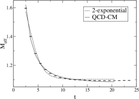
Figure 1: Plot of the effective mass for the $\kappa=0.1385$ case. The result of a 2-exponential fit together with the QCD Continuum Model fits of Eq.(7) & Eq.(9) are shown. (The latter two fits are indistinguishable on the plot by eye.)

3 Analytic lattice results for non-degenerate mesons

In Section 2, an analytic expression for the 2-point function $G_{2}$ was derived by using the continuum, short-distance expansion for the quark propagator, $S_{q}$. In this section we extend this work still further using the lattice expression for (the co-ordinate space) quark propagator, $S_{q}(x)^{LAT}$, recently derived by Paladini for Wilson quarks[4].

While the momentum space expression for lattice propagators has a simple, closed form, the co-ordinate space representation does not. Before the work of [4], $S_{q}(x)^{LAT}$ was known in two cases only: the massless limit [5]; and the $x=0$ limit [6].

In [4], $S_{q}(x)^{W}$ (for Wilson Quarks) was derived as a continuum expansion (i.e. as a Taylor expansion in the lattice spacing, $a$). To obtain this expression the authors of [4] used a special asymptotic series they developed for the modified Bessel functions which appear in the standard form of $S_{q}(x)^{LAT}$. Their result, expressed to ${\cal O}(a)$ is,

$$(4\pi)^{2}S_{q}(x)^{W}\!\!\! = \!\!\!\frac{4m^{2}}{(x^{2})^{\frac{1}{2}}}\left(1+\frac{ram}{2}\right)K_{1}\left[m(x^{2})^{\frac{1}{2}}\right]$$ (8)

$$+ \!\!\!2ram^{4}K_{2}\left[m{(x^{2})}^{\frac{1}{2}}\right]$$

$$+ \!\!\!2ram^{4}\frac{\gamma\cdot x}{(x^{2})^{\frac{1}{2}}}K_{1}\left[m{(x^{2})}^{\frac{1}{2}}\right]$$

$$+ \!\!\!4m^{2}(1+ram)\frac{\gamma\cdot x}{x^{2}}K_{2}\left[m{(x^{2})}^{\frac{1}{2}}\right]$$

$$+ \!\!\!\mathcal{O}(\mathit{a^{2}}),$$

where $K_{1}$ and $K_{2}$ are modified Bessel functions of the second kind.

In [7], $S_{q}(x)^{W}$ was used instead of Eq.(1) in Eq.(3) thereby obtaining an expression for $G_{2}(t)$ for Wilson fermions correct to ${\cal O}(a)$. [7] lists results for all of the commonly used mesonic channels. Here we list only the result for the vector channel:

$$G_{2}^{Vi}(t)^{OPE,W} = \frac{-1}{2\pi^{2}t^{3}}[1+ra(m_{1}+m_{2})]$$ (9)

$$+ \frac{3}{8\pi^{2}t}[m_{1}^{2}+m_{2}^{2}-2m_{1}m_{2}$$

$$+2ra(m_{1}m_{2}^{2}+m_{1}^{2}m_{2})],$$

where $r$ is the Wilson parameter. Note that, as expected, $G_{2}^{OPE,W}=G_{2}^{OPE,cont}+{\cal O}(a)$.

Table 2 shows the results for the lattice-QCD Continuum Model fit, Eq.(9). In this table the $\chi^{2}$ values are shown together with the estimates of the $Z$ and $M$ values. The lattice-QCD Continuum Model fits are very similar to the QCD Continuum Model fits from Eq.(7), but they become significantly better (i.e. have a smaller $\chi^{2}$) as the quark mass increases. This is to be expected since the lattice artefacts $\sim ma$. (Note that in Figure 1 where the effective mass for the vector channel at $\kappa_{1,2}=0.1385$ is plotted, the results from the fit to Eq.(9) is indistinguishable by eye to that from Eq.(7).)

4 Maximum Entropy Method and the Nambu–Jona-Lasinio Model

In the above two sections, an Ansatz for the spectral function $\rho(s)$ was derived using an analytic expression for the quark propagator, $S_{q}(x)$, valid at small $x$. This Ansatz was then used as a fitting function for Monte Carlo data for 2-point hadronic functions, $G_{2}(t)$. It is interesting to ponder if $\rho(s)$ itself can be directly extracted from Monte Carlo $G_{2}(t)$ data.

At first sight this aim appears impossible to achieve due to the intrinsic ambiguity in the inversion. $G_{2}(t)$ is known at $N_{t}\approx{\cal O}(10)$ values of $t$ whereas, in order to reveal spectral structure, $\rho(s)$ must be calculated at $N_{s}\;\raisebox{-2.15277pt}{\hbox to0.0pt{$\sim$\hss}}\raisebox{2.15277pt}{$>$}\;{\cal O}(100)$ $s$ values. This means that there are an infinite number of solutions for $\rho(s)$ which perfectly fit the data $G_{2}(t)$.

In [8] the Maximum Entropy Method (which is well known in almost every numerical field outside lattice gauge theory!) was used to overcome this seemingly insurmountable problem. Bayes’ theorem can be used to express the probability of $\rho(s)$ given the data $G_{2}(t)$, $P(\rho|G_{2})$, as

$$P(\rho|G_{2})\propto P(G_{2}|\rho)\times P(\rho).$$ (10)

Here, $P(G_{2}|\rho)$ can be written as the usual exponential of the standard $\chi^{2}$ function of the Maximum Likelyhood Method. The probability, $P(\rho)$ can be expressed in terms of the entropy function, $S$. The best solution for $\rho$ is obtained by “just” maximising $P(\rho|G_{2})$ in Eq.(10).

Since the work of [8] there have been several applications of the MEM method to lattice simulations. In this paper, we concentrate on applying the MEM to the Nambu–Jona-Lasinio model in (2+1)D. This work is discussed in more detail in [9]. For details of applying MEM to lattice simulations see [8].

The continuum (Euclidean) NJL Lagrangian is:

$${\cal L}=\bar{\Psi}_{i}(\partial\hskip-5.0pt/+m_{0}+\sigma+i\gamma_{5}\pi)\Psi_{i}+\frac{N_{f}}{2g^{2}}(\sigma^{2}+\pi^{2}).$$

The fields $\Psi_{i}$ and $\bar{\Psi}_{i}$ are four-component spinors and the index $i$ runs over $N_{f}$ fermion flavours. The model has an interacting continuum limit and has been used to model the strong interaction. It exists in two phases defined by a chiral order parameter. The lattice simulation used the staggered fermion formulation.

Figure 2 shows the spectral function obtained from MEM for the $\pi$, fermion (f) and massive PS meson in the broken phase with $N_{f}=4$ flavours and coupling of $\beta=1/g^{2}=0.55$. This plot represents approximately 30,000 configurations of data. It shows that MEM is easily able to isolate the ground states in these channels. Furthermore, estimates of the binding energy of the PS state can be obtained using the MEM spectral functions which are in agreement with expectations from large $N_{f}$ expansions [9].

In Figure 3, the $\pi$ mass squared is plotted against the quark mass showing that the PCAC scaling relationship holds.

Further results for both phases are detailed in [9] and future work where MEM is applied to the UKQCD dynamical data set is detailed in [10].

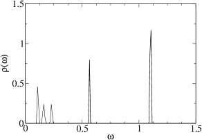
Figure 2: Broken phase spectral functions for the NJL model. Peaks from left to right are for the $\pi$ ($m_{0}=0.005,0.01,0.02$), f and PS (both $m_{0}=0.01$).

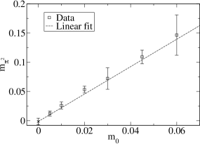
Figure 3: PCAC scaling relation for $\beta=0.55$ NJL data sets.

5 Conclusions

This paper summarises the results from two interesting “unconventional” approaches to the study of 2-point hadronic correlation functions in lattice Monte Carlo simulations, $G_{2}(t)$. The first approach aims at obtaining an accurate analytic expression for the short distance behaviour of $G_{2}(t)$ via the QCD Sum Rules Continuum Model. In particular, the recently derived expression for the Wilson quark propagator [4] was used. Further work in this area will include the derivation of the analytic expression for the clover quark propagator and, from that, the calculation of the analogous expression for $G_{2}(t)$ at short distances for this action.

The second approach uses the Maximum Entropy Method to calculate the spectral function, $\rho(s)$, given the 2-point function, $G_{2}(t)$. This technique is being used by a growing number of researchers in this context. In this work we used MEM to study the Nambu–Jona-Lasinio model and found it to work admirably.

6 Acknowledgements

The authors wish to thank Simon Hands, Craig McNeile and Costas Strouthos for invaluable help and they acknowledge the UKQCD Collaboration for use of Cray T3E resources.

References

- [1] D. Leinweber, Phys.Rev. D51 (1995) 6369-6382.
- [2] C.R. Allton and S. Capitani, Nucl. Phys. B526 (1998) 463-486.
- [3] D. Blythe hep-lat/0111016; C.R. Allton, D. Blythe, J. Clowser, work in progress
- [4] B.M.S. Paladini, Ph.D. Thesis, Trinity College Dublin; B.M.S. Paladini and J. Sexton, Phys.Lett. B448 (1999) 76-84.
- [5] M. Lüscher and P. Weisz, Nucl. Phys. B445 (1995) 429-450.
- [6] Burgio, Caracciolo and Pelisetto, Nucl.Phys. B478 (1996) 687-722.
- [7] D. Blythe, C.R. Allton and C. McNeile, work in progress
- [8] Y. Nakahara, M. Asakawa and T. Hatsuda, Phys. Rev. D60 (1999) 091503; Prog.Part.Nucl.Phys. 46 (2001) 459.
- [9] J. Clowser and C. Strouthos, hep-lat/0110136; C. Strouthos, J. Clowser, S.J. Hands, J. Kogut, C.R. Allton work in progress;
- [10] J. Clowser and C.R. Allton, work in progress