Overlap Quark Propagator in Landau Gauge

Abstract

The properties of the quark propagator in Landau gauge in quenched QCD are examined for the overlap quark action. The overlap quark action satisfies the Ginsparg-Wilson relation and as such provides an exact lattice realization of chiral symmetry. This in turn implies that the quark action is free of ${\cal O}(a)$ errors. We present results using the standard Wilson fermion kernel in the overlap formalism on a $12^{3}\times 24$ lattice at a spacing of 0.125 fm. We obtain the nonperturbative momentum-dependent wavefunction renormalization function $Z(p)$ and the nonperturbative mass function $M(p)$ for a variety of bare masses. We perform a simple extrapolation to the chiral limit for these functions. We clearly observe the dynamically generated infrared mass and confirm the qualitative behavior found for the Landau gauge quark propagator in earlier studies. We attempt to extract the quark condensate from the asymptotic behavior of the mass function in the chiral limit.

I INTRODUCTION

Hadron correlators on the lattice provide a direct means of calculating the physically observable properties of quantum chromodynamics (QCD). They are by construction color-singlet (i.e., gauge-invariant) quantities. Any finite, Boltzmann-distributed ensemble of gauge configurations has negligible probability of containing two gauge-equivalent configurations. Hence, there is a negligible probability of any gauge orbit being represented more than once in the Monte-Carlo estimate of the color-singlet hadron-correlator and this is the reason that there is no need to gauge fix in such calculations.

On the other hand, calculations of high-energy processes are carried out analytically with perturbative QCD, where it is necessary to select a gauge. Quark models and QCD-inspired Dyson-Schwinger equation models[1] are necessarily formulated in a particular gauge. The usual Fadeev-Popov gauge-fixing procedure is adequate for perturbative QCD. However in the nonperturbative infrared region standard gauge choices, such as Landau gauge, have Gribov copies, i.e., there are multiple gauge configurations on a given gauge orbit which satisfy the gauge-fixing condition. Since no finite ensemble will ever contain two configurations from the same gauge orbit, Landau gauge on the lattice actually corresponds to a gauge where there is a more or less random choice between the Landau gauge Gribov copies on the represented gauge orbits in the ensemble. Before gauge fixing, the ensemble contains configurations randomly located on their gauge orbits. After Landau gauge fixing on the lattice each configuration in the ensemble will typically settle on one of the nearby Landau gauge Gribov copies. This is the standard lattice implementation of Landau gauge and the one that we consider in this work.

In order to study the transition from non-perturbative to the perturbative regime on the lattice we can study the gluon[2] and quark[3, 4, 5, 6] propagators and vertices such as the quark-gluon vertex[10]. By studying the momentum dependent quark mass function in the infrared region we can gain some insights into the mechanism of dynamical chiral symmetry breaking and the associated dynamical generation of mass. Studying the ultraviolet behaviour of propagators at large momentum is made difficult because of lattice artifacts causing the propagator to deviate strongly from its correct continuum behaviour in this regime. The method of tree-level correction was developed and used successfully in gluon propagator studies[2] and has recently been extended to the case of the quark propagator[4, 5, 6]. Some related studies have been performed for the case of domain-wall fermions[7]. Detailed discusions of nonpertubative renormalization for lattice operators can be found, e.g., in Refs. [8, 9]

We present here results for the quark propagator obtained from the overlap quark action and using an improved gauge action and improved Landau gauge fixing. The overlap action is an exact realization of chiral symmetry on the lattice and is necessarily ${\cal O}(a)$-improved. In Secs. II and III we briefly introduce the improved gauge action and the lattice quark propagator respectively. In Sec. IV we introduce the overlap quark propagator and describe how it is calculated. Our numerical results are presented in Sec. V and finally in Sec. VI we give our summary and conclusions.

II IMPROVED GAUGE ACTION

The tree-level ${\cal O}(a^{2})$-improved action is defined as,

$$S_{G}=\frac{5\beta}{3}\sum_{\scriptstyle x\,\mu\,\nu\atop\scriptstyle\nu>\mu}{\rm Re\,tr}(1-P_{\mu\nu}(x))-\frac{\beta}{12\,u_{0}^{2}}\sum_{\scriptstyle x\,\mu\,\nu\,\atop\scriptstyle\nu>\mu}{\rm Re\,tr}(1-R_{\mu\nu}(x)),$$ (1)

where $P_{\mu\nu}$ and $R_{\mu\nu}$ are defined as

$$P_{\mu\nu}(x) = U_{\mu}(x)\,U_{\nu}(x+{\hat{\mu}})\,U^{\dagger}_{\mu}(x+{\hat{\nu}})U^{\dagger}_{\nu}(x),$$ (2)

$$R_{\mu\nu}(x) = U_{\mu}(x)\,U_{\nu}(x+{\hat{\mu}})\,U_{\nu}(x+{\hat{\nu}}+{\hat{\mu}})\,U^{\dagger}_{\mu}(x+2{\hat{\nu}})\,U^{\dagger}_{\nu}(x+{\hat{\nu}})\,U^{\dagger}_{\nu}(x)$$ (3)

$$+ U_{\mu}(x)\,U_{\mu}(x+{\hat{\mu}})\,U_{\nu}(x+2{\hat{\mu}})\,U^{\dagger}_{\mu}(x+{\hat{\mu}}+{\hat{\nu}})\,U^{\dagger}_{\mu}(x+{\hat{\nu}})\,U^{\dagger}_{\nu}(x).$$ (4)

The link product $R_{\mu\nu}(x)$ denotes the rectangular $1\times 2$ and $2\times 1$ plaquettes. The mean link, $u_{0}$, is the tadpole (or mean-field) improvement factor that largely corrects for the quantum renormalization of the coefficient for the rectangles relative to the plaquette. We employ the plaquette measure for the mean link

$$u_{0}=\left(\frac{1}{3}{\rm Re\,tr}\left<P_{\mu\nu}(x)\right>\right)^{1/4}\,,$$ (5)

where the angular brackets indicate averaging over $x$, $\mu$, and $\nu$.

Gauge configurations are generated using the Cabbibo-Marinari [11] pseudo–heat–bath algorithm with three diagonal $SU_{c}(2)$ subgroups cycled twice. Simulations are performed using a parallel algorithm on a Sun Cluster composed of 40 nodes and on a Thinking Machines Corporations (TMC) CM-5 both with appropriate link partitioning. We partition the link variables according to the algorithm described in Ref. [12]. We use 50 configurations generated on a $12^{3}\times{24}$ lattice at $\beta=4.60$, selected after 5000 thermalization sweeps from a cold start and every 500 sweeps thereafter with a fixed mean–link value. Lattice parameters are summarized in Table I. The lattice spacing is determined from the static quark potential with a string tension $\sqrt{\sigma}=440$ MeV[13].

TABLE I.: Lattice parameters.

Action	Volume	$N_{\rm{Therm}}$	$N_{\rm{Samp}}$	$\beta$	$a$ (fm)	$u_{0}$	Physical Volume (fm4)
Improved	$12^{3}\times{24}$	5000	500	4.60	0.125	0.88888	$1.5^{3}\times{3.00}$

The gauge field configurations are gauge fixed to the Landau gauge using a Conjugate Gradient Fourier Acceleration [14] algorithm with an accuracy of $\theta\equiv\sum\left|\partial_{\mu}A_{\mu}(x)\right|^{2}<10^{-12}$. We use an improved gauge-fixing scheme to minimize gauge-fixing discretization errors. A discussion of the functional and method for improved Landau gauge fixing can be found in Ref. [15].

III Quark Propagator on the Lattice

In a covariant gauge in the continuum the renormalized Euclidean space quark propagator must have the form

$$S(\zeta;p)=\frac{1}{i{p\!\!\!/}A(\zeta;p^{2})+B(\zeta;p^{2})}=\frac{Z(\zeta;p^{2})}{i{p\!\!\!/}+M(p^{2})}\,,$$ (6)

where $\zeta$ is the renormalization point and where the renormalization point boundary conditions are $Z(\zeta;\zeta^{2})\equiv 1$ and $M(\zeta^{2})\equiv m(\zeta)$ and where $m(\zeta)$ is the renormalized quark mass at the renormalization point. Since the gauge fixing condition has no preferred direction in color space, the quark propagator must be diagonal in color space, i.e., $S^{ij}(\zeta;p)=S(\zeta;p)\delta^{ij}$ where $\delta^{ij}$ is the $3\times 3$, $SU(3)_{c}$ identity matrix. The functions $A(\zeta;p^{2})$ and $B(\zeta;p^{2})$, or alternatively $Z(\zeta;p^{2})$ and $M(p^{2})$, contain all of the nonperturbative information of the quark propagator. Note that $M(p^{2})$ is renormalization point independent, i.e., since $S(\zeta;p)$ is multiplicatively renormalizable all of the renormalization-point dependence is carried by $Z(\zeta;p^{2})$. For sufficiently large momenta the effects of dynamical chiral symmetry breaking become negligible for nonzero current quark masses, i.e., for large $\zeta$ and $m_{\zeta}\neq 0$ we have $m(\zeta)\to m_{\zeta}$ where $m_{\zeta}$ is the usual current quark mass of perturbative QCD at the renormalization point $\zeta$. When all interactions for the quarks are turned off, i.e., when the gluon field vanishes, the quark propagator has its tree-level form

$$S^{(0)}(p)=\frac{1}{i{p\!\!\!/}+m^{0}}\,,$$ (7)

where $m^{0}$ is the bare quark mass. When the interactions with the gluon field are turned on we have

$$S^{(0)}(p)\to S^{\rm bare}(a;p)=Z_{2}(\zeta;a)S(\zeta;p)\,,$$ (8)

where $a$ is the regularization parameter (i.e., the lattice spacing here) and $Z_{2}(\zeta;a)$ is the quark wave-function renormalization constant chosen so as to ensure $Z(\zeta;\zeta^{2})=1$. For simplicity of notation we suppress the $a$-dependence of the bare quantities.

On the lattice we expect the bare quark propagators, in momentum space, to have a similar form as in the continuum [3, 4, 5], except that the $O(4)$ invariance is replaced by a 4-dimensional hypercubic symmetry on an isotropic lattice. Hence, the inverse lattice bare quark propagator takes the general form

$$(S^{\rm bare})^{-1}(p)\equiv{i\left(\sum_{\mu}C_{\mu}(p)\gamma_{\mu}\right)+B(p)}.$$ (9)

We use periodic boundary conditions in the spatial directions and anti-periodic in the time direction. The discrete momentum values for a lattice of size $N^{3}_{i}\times{N_{t}}$, with $n_{i}=1,..,N_{i}$ and $n_{t}=1,..,N_{t}$, are

$$p_{i}=\frac{2\pi}{N_{i}a}\left(n_{i}-\frac{N_{i}}{2}\right),\hskip 28.45274pt{\rm{and}}\hskip 28.45274ptp_{t}=\frac{2\pi}{N_{t}a}\left(n_{t}-\frac{1}{2}-\frac{N_{t}}{2}\right).$$ (10)

Defining the bare lattice quark propagator as

$$S^{\rm bare}(p)\equiv{-i\left(\sum_{\mu}{\cal{C}}_{\mu}(p)\gamma_{\mu}\right)+{\cal{B}}(p)}\,,$$ (11)

we perform a spinor and color trace to identify

$${\cal{C}}_{\mu}(p)=\frac{i}{4N_{c}}{\rm tr}[\gamma_{\mu}{S^{\rm bare}(p)}]\hskip 28.45274pt {\rm{and}} \hskip 28.45274pt{\cal{B}}(p)=\frac{1}{4N_{c}}{\rm tr}[S^{\rm bare}(p)]\,.$$ (12)

The inverse propagator is

$$(S^{\rm bare})^{-1}(p) = \frac{1}{{-i\left(\sum_{\mu}{\cal{C}}_{\mu}(p)\gamma_{\mu}\right)+{\cal{B}}(p)}}$$ (13)

$$= \frac{{i\left(\sum_{\mu}{\cal{C}}_{\mu}(p)\gamma_{\mu}\right)+{\cal{B}}(p)}}{{\cal{C}}^{2}(p)+{\cal{B}}^{2}(p)}\,,$$ (14)

where ${\cal{C}}^{2}(p)=\sum_{\mu}({\cal{C}}_{\mu}(p))^{2}$. From Eq. (9) we identify

$$C_{\mu}(p)=\frac{{\cal{C}}_{\mu}(p)}{{\cal{C}}^{2}(p)+{\cal{B}}^{2}(p)}\hskip 28.45274pt{\rm{and}}\hskip 28.45274ptB(p)=\frac{{\cal{B}}(p)}{{\cal{C}}^{2}(p)+{\cal{B}}^{2}(p)}\,.$$ (15)

A Tree-level correction

At tree–level, i.e., when all the gauge links are set to the identity, the inverse bare lattice quark propagator becomes the tree-level version of Eq. (9)

$$(S^{(0)})^{-1}(p)\equiv{i\left(\sum_{\mu}C_{\mu}^{(0)}(p)\gamma_{\mu}\right)+B^{(0)}(p)}\,.$$ (16)

We calculate $(S^{(0)})(p)$ directly by setting the links to unity in the coordinate space quark propagator and taking its Fourier transform

It is then possible to identify the appropriate kinematic lattice momentum directly from the definition

$$q_{\mu}\equiv C_{\mu}^{(0)}(p) = \frac{{\cal{C}}_{\mu}^{(0)}(p)}{({\cal{C}}^{(0)}(p))^{2}+({\cal{B}}^{(0)}(p))^{2}}\,.$$ (17)

This is the starting point for the general approach to tree-level correction developed in earlier studies of the gluon propagator[2] and the quark propagator[4, 5, 6].

Having identified the appropriate kinematical lattice momentum $q$, we can now define the bare lattice propagator as

$$S^{\rm bare}(p)\equiv\frac{1}{i{q\!\!\!/}A(p)+B(p)}=\frac{Z(p)}{i{q\!\!\!/}+M(p)}=Z_{2}(\zeta;a)S(\zeta;p)$$ (18)

and the lattice version of the renormalized propagator in Eq. (6)

$$S(\zeta;p)\equiv\frac{1}{i{q\!\!\!/}A(\zeta;p)+B(\zeta;p)}=\frac{Z(\zeta;p)}{i{q\!\!\!/}+M(p)}\,.$$ (19)

The general approach to tree-level correction[2, 4, 5, 6] utilizes the fact that QCD is asymptotically free and so it is the difference of bare quantities from their tree-level form on the lattice that contains the best estimate of the nonperturbative information. For example, multiplicative tree-level correction for $Z(p)$ and $M(p)$ has the form

$$Z^{(c)}(p)=\frac{Z(p)}{Z^{(0)}(p)}1\hskip 28.45274pt{\rm{and}}\hskip 28.45274ptM^{(c)}(p)=\frac{M(p)}{M^{(0)}(p)}m^{0}\,.$$ (20)

The identification of the kinematical variable $q$ ensures that $A^{\rm(0)}(p)=1/Z^{\rm(0)}(p)=1$ by construction and so $Z(p)=Z^{(c)}(p)$ and is already tree-level corrected. For overlap quarks we will see that $M^{(0)}(p)=m^{0}$ and so the mass function satisfies $M(p)=M^{(c)}(p)$ and needs no tree-level correction either. This feature is a major advantage of the overlap formalism.

IV OVERLAP FERMIONS.

The overlap fermion formalism [16, 17, 18, 19, 20, 21, 22, 23, 24, 25] realizes an exact chiral symmetry on the lattice and is automatically ${\cal O}(a)$ improved, since any ${\cal O}(a)$ error would necessarily violate chiral symmetry[20]. The massless coordinate-space overlap-Dirac operator can be written in dimensionless lattice units as[21]

$$D(0)=\frac{1}{2}\left[1+\gamma_{5}H_{a}\right]\,,$$ (21)

where $H_{a}$ is an Hermitian operator that depends on the background gauge field and has eigenvalues $\pm 1$. Any such $D(0)$ is easily seen to satisfy the Ginsparg–Wilson relation [27]

$$\{\gamma_{5},D(0)\}=2D(0)\gamma_{5}D(0)$$ (22)

and, provided that its Fourier transform at low momenta is proportional to the momentum-space covariant derivative, it will satisfy a deformed lattice realization of chiral symmetry. It immediately follows from Eq. (21) that

$$D^{\dagger}(0)D(0)=D(0)D^{\dagger}(0)=\frac{1}{2}[D^{\dagger}(0)+D(0)]$$ (23)

and that

$$D^{\dagger}(0)=\gamma_{5}D(0)\gamma_{5}\,.$$ (24)

It also follows easily that $\{\gamma_{5},D^{-1}(0)\}=2\gamma_{5}$ and by defining $\tilde{D}^{-1}(0)\equiv[D^{-1}(0)-1]$ we see that the Ginsparg-Wilson relation can also be expressed in the form

$$\{\gamma_{5},\tilde{D}^{-1}(0)\}=0\,.$$ (25)

The standard choice of $H_{a}(x,y)$ is $H_{a}=\epsilon(H_{w})\equiv H_{w}/|H_{w}|=H_{w}/(H_{w}^{\dagger}H_{w})^{1/2}$, where $H_{w}(x,y)=\gamma_{5}D_{w}(x,y)$ is the Hermitian Wilson-Dirac operator and where $D_{w}$ is the usual Wilson-Dirac operator on the lattice. However, in the overlap formalism the Wilson mass parameter $m_{w}$ is the negative of what it is for standard Wilson fermions and at tree-level must satisfy $0<m_{w}a<2$. In the overlap formalism $m_{w}$ is an intermediate lattice regularization parameter, it is not the bare quark mass. When interactions are present, we must have $m_{1}a<m_{w}a$ in order that the Wilson operator has zero-crossings and, in turn, that $D(0)$ has nontrivial topological charge. Numerical studies have found that $m_{1}\simeq m_{c}$, where $m_{c}$ is the usual critical mass for Wilson fermions[26]. The constraint $m_{w}a<2$ at tree level arises from the fact that Wilson doublers reappear above this point. In summary, we use here $H_{w}(-m_{w})=\gamma_{5}\,D_{w}(-m_{w})$.

Recall that the standard Wilson-Dirac operator can be written as

$$D_{w}(x,y) = \left[(-m_{w}a)+4r\right]\delta_{x,y}-\frac{1}{2}\sum_{\mu}\left\{(r-\gamma_{\mu})U_{\mu}(x)\delta_{y,x+\hat{\mu}}+(r+\gamma_{\mu})U^{\dagger}_{\mu}(x-a\hat{\mu})\delta_{y,x-\hat{\mu}}\right\}$$ (26)

$$= \frac{1}{2\kappa^{\rm st}}\left[\delta_{x,y}-\kappa^{\rm st}\sum_{\mu}\left\{(r-\gamma_{\mu})U_{\mu}(x)\delta_{y,x+\hat{\mu}}+(r+\gamma_{\mu})U^{\dagger}_{\mu}(x-a\hat{\mu})\delta_{y,x-\hat{\mu}}\right\}\right]\,,$$ (27)

where the negative Wilson mass term $(-m_{w}a)$ is then defined by $(-m_{w}a)+4r=1/2\kappa^{\rm st}$ or equivalently

$$\kappa^{\rm st}\equiv\frac{1}{2(-m_{w}a)+(1/\kappa_{c})}$$ (28)

and where $\kappa_{c}$ throughout this work is the tree-level critical $\kappa$, i.e., $\kappa_{c}=1/(8r)$.

In the present work we use the mean-field improved Wilson-Dirac operator, which can be written as

$$D_{w}(x,y)=\frac{u_{0}}{2\kappa}\left[\delta_{x,y}-\kappa\sum_{\mu}\left\{(r-\gamma_{\mu})\frac{U_{\mu}(x)}{u_{0}}\delta_{y,x+\hat{\mu}}+(r+\gamma_{\mu})\frac{U^{\dagger}_{\mu}(x-a\hat{\mu})}{u_{0}}\delta_{y,x-\hat{\mu}}\right\}\right]\,.$$ (29)

We see that this is equivalent to the standard Wilson-Dirac operator with the identification of the mean-field improved coefficient $\kappa\equiv\kappa^{\rm st}u_{0}$. It is $U/u_{0}$ that has a more convergent expansion around the identity than the links $U$ themselves. The negative Wilson mass $(-m_{w}a)$ is then related to this improved $\kappa$ by

$$\kappa\equiv\frac{u_{0}}{2(-m_{w}a)+(1/\kappa_{c})}\,.$$ (30)

The Wilson parameter is typically chosen to be $r=1$ and we will also use $r=1$ here in our numerical simulations.

For this mean-field improved Wilson-Dirac choice we then have

$$D(0)=\frac{1}{2}\left[1+D_{w}\left(D_{w}^{\dagger}D_{w}\right)^{-1/2}\right]\,.$$ (31)

In coordinate space the Wilson-Dirac operator has the form $D_{w}=\nabla\!\!\!\!/+(r/2)\Delta+(-m_{w}a)$, where $\nabla_{\mu}$ is the symmetric dimensionless lattice finite difference operator, and $\Delta$ is the dimensionless lattice Laplacian operator. Recall that the Wilson mass term is $(-m_{w}a)$ here. Setting the links to the identity gives

$$D_{w}=(1/2)(\stackrel{{\scriptstyle\leftarrow}}{{\partial}}_{\mu}+\stackrel{{\scriptstyle\rightarrow}}{{\partial}}_{\mu})\gamma_{\mu}+(r/2)(-\stackrel{{\scriptstyle\leftarrow}}{{\partial}}_{\mu}\stackrel{{\scriptstyle\rightarrow}}{{\partial}}_{\mu})+(-m_{w}a)\,,$$ (32)

where the partial derivatives are the forward and backward lattice finite difference operators. Hence we have from Eq. (31) that

$$D(0) = \frac{1}{2}\left[1+\frac{\nabla\!\!\!\!/+(r/2)\Delta-m_{w}a}{\sqrt{(m_{w}a)^{2}+{\cal O}(\partial^{2})}}\right]$$ (33)

$$\to \frac{\nabla\!\!\!\!/}{2m_{w}a}\,,$$ (34)

where the last line is a limit approached when operating on very smooth functions such that only first powers of derivatives are kept. The reason for needing a negative Wilson mass $(-m_{w}a)$ is now apparent, i.e., it is needed to cancel the 1 in $D(0)$. We see that at sufficiently fine lattice spacings and for $pa\ll 1$

$$D_{c}(0)\equiv(2m_{w})D(0)\,,$$ (35)

where $D_{c}(0)$ in the continuum limit becomes the usual fermion covariant derivative contracted with the $\gamma$-matrices, i.e., $D_{c}(0)\to D\!\!\!\!/$ as $a\to 0$.

The massless overlap quark propagator is given by

$$S^{\rm bare}(0)\equiv\tilde{D}_{c}^{-1}(0)\equiv D_{c}^{-1}(0)-\frac{1}{2m_{w}}=\frac{1}{2m_{w}}\left[D^{-1}(0)-1\right]=\frac{1}{2m_{w}}\tilde{D}^{-1}(0)\,.$$ (36)

This definition of the massless overlap quark propagator follows from the overlap formalism[19] and ensures that the massless quark propagator anticommutes with $\gamma_{5}$, i.e., $\{\gamma_{5},S^{\rm bare}(0)\}=0$ just as it does in the continuum [21]. At tree-level the momentum-space form of the massless propagator defines the kinematic lattice momentum $q$, i.e., we set the links to one such that we have for the momentum-space massless quark propagator

$$S^{\rm bare}(0,p)\equiv\tilde{D}_{c}^{-1}(0,p)\to S^{(0)}(0,p)=\frac{1}{iq\!\!\!/}\,,$$ (37)

where recall that $p$ is the discrete lattice momentum defined in Eq. (10) and $q$ is the kinematical lattice momentum defined in Eq. (17). We can obtain $q$ numerically in this way from the tree-level massless quark propagator. We can compare this with the analytic form for $q$ derived in the Appendix and given in Eq. (A12).

Note that for our mean-field improved Wilson-Dirac operator, the tree-level limit for defining $q$ implies that we should take $U\to I$ and $u_{0}\to 1$ in $D_{w}$ while keeping $\kappa$ fixed. Thus the $\kappa$ that appears in the tree-level expression for $q_{\mu}$ in Eq. (A12) is actually the improved $\kappa$ and not $\kappa^{\rm st}$. This means that the tree-level Wilson mass parameter, $m_{w}^{(0)}$, used in the Appendix is given by $\kappa=1/[2(-m_{w}^{(0)}a)+(1/\kappa_{c})]$ and hence differs from the $m_{w}$ in Eq. (30) used in the main body of the paper. We have found that the $q$ obtained in this way gives a much superior large momentum behavior for the $M(p)$ and $Z(p)$ functions than is obtained when we do not use mean-field improvement.

Having identified the massless quark propagator in Eq. (36), we can construct the massive overlap quark propagator by simply adding a bare mass to its inverse,i.e.,

$$(S^{\rm bare})^{-1}(m^{0})\equiv(S^{\rm bare})^{-1}(0)+m^{0}\,.$$ (38)

Hence, at tree-level we have for the massive, momentum-space overlap quark propagator

$$S^{\rm bare}(m^{0},p)\to S^{(0)}(m^{0},p)=\frac{1}{iq\!\!\!/+m^{0}}$$ (39)

and the reason that the overlap quark propagator needs no tree-level correction beyond identifying $q$ is now clear.

In order to complete the discussion we now relate our presentation to standard notation used elsewhere. We first define the dimensionless overlap mass parameter

$$\mu\equiv\frac{m^{0}}{2m_{w}}$$ (40)

and then define $\tilde{D}_{c}^{-1}(\mu)$ in analogy with Eq. (36)

$$S^{\rm bare}(m^{0})\equiv\tilde{D}_{c}^{-1}(\mu)\,,$$ (41)

i.e., $\tilde{D}_{c}^{-1}(\mu)$ is a generalization of $\tilde{D}_{c}^{-1}(0)$ to the case of nonzero mass. Extending the analogy with the massless case we introduce $\tilde{D}(\mu)$ and $D(\mu)$, which are generalized versions of $\tilde{D}(0)$ and $D(0)$, through the definitions

$$\tilde{D}_{c}^{-1}(\mu)\equiv\frac{1}{2m_{w}}\tilde{D}^{-1}(\mu)\hskip 28.45274pt{\rm{and}}\hskip 28.45274pt\tilde{D}^{-1}(\mu)\equiv\frac{1}{1-\mu}\left[{D}^{-1}(\mu)-1\right]\,.$$ (42)

We can now use Eq. (38) and the above definitions to obtain an expression for $D(\mu)$. From Eqs. (38), (40) and (42) we see that we must have $\tilde{D}(\mu)=\tilde{D}(0)+\mu$. Inverting this gives

$$\frac{1}{1-\mu}\left[D^{-1}(\mu)-1\right]=\left[\tilde{D}(0)+\mu\right]^{-1}$$ (43)

and so

$$D^{-1}(\mu)=(1-\mu)\left[\tilde{D}(0)+\mu\right]^{-1}+1=\left[\tilde{D}(0)+1\right]\left[\tilde{D}(0)+\mu\right]^{-1}\,.$$ (44)

Inverting gives

$$D(\mu)=\left[\tilde{D}(0)+\mu\right]\left[\tilde{D}(0)+1\right]^{-1}\hskip 28.45274pt{\rm{and~{}also}}\hskip 28.45274ptD(0)=\tilde{D}(0)\left[\tilde{D}(0)+1\right]^{-1}$$ (45)

and so finally

$$D(\mu) = \left[(1-\mu)\tilde{D}(0)+\mu\left(\tilde{D}(0)+1\right)\right]\left[\tilde{D}(0)+1\right]^{-1}$$ (46)

$$= (1-\mu)D(0)+\mu=\frac{1}{2}\left[1+\mu+(1-\mu)\gamma_{5}H_{a}\right]\,.$$ (47)

We have then recovered the standard expression for $D(\mu)$ found for example in Ref. [21] and elsewhere.

We see that the massless limit, $m^{0}\to 0$, implies that $\mu\to 0$ and $D(\mu)\to D(0)$, $\tilde{D}^{-1}(\mu)\to\tilde{D}^{-1}(0)$ and $\tilde{D}_{c}^{-1}(\mu)\to\tilde{D}_{c}^{-1}(0)$. For non-negative bare mass $m^{0}$ we require $\mu\geq 0$. In order that the above expressions and manipulations be well-defined we must have $\mu<1$. Hence, $0\leq\mu<1$ defines the allowable range of bare masses.

Our numerical calculation begins with an evaluation of the inverse of $D(\mu)$, where $D(\mu)$ is defined in Eq. (47) and using $H_{a}=\epsilon(H_{w})$ for each gauge configuration in the ensemble. We then calculate Eq. (41) for each configuration and take the ensemble average to obtain $S^{\rm bare}(x,y)$. The discrete Fourier transform of this finally gives the momentum-space bare quark propagator, $S^{\rm bare}(p)$, for the bare quark mass $m^{0}$.

Our calculations used $\kappa=0.19$ and $u_{0}=0.88888$ and since at tree level $\kappa_{c}=1/8$, we then have $m_{w}a=1.661$. Recall that the lattice spacing is $a=0.125$ fm and so we have $a^{-1}=1.58$ GeV and $m_{w}=2.62$ GeV. We calculated at ten quark masses specified by $\mu=$ $0.024$, $0.028$, $0.032$, $0.040$, $0.048$, $0.060$, $0.080$, $0.100$, $0.120$, and $0.140$. This corresponds to bare masses in physical units of $m^{0}=2\mu m_{w}=$ $126$, $147$, $168$, $210$, $252$, $315$, $420$, $524$, $629$, and $734$ MeV respectively.

V NUMERICAL RESULTS

We have numerically extracted the kinematical lattice momentum $q_{\mu}$ directly from the tree-level overlap propagator using Eqs. (12), (15) and (17). In particular, by setting $U\to I$ and $u_{0}\to 1$ we have numerically verified to high-precision the tree-level behavior in Eq. (39) for all ten of our bare masses $m^{0}$, which is a good test of our code for extracting the momentum-space quark propagator. We plot $q\equiv\sqrt{\sum_{\mu}q_{\mu}^{2}}$ against the discrete lattice momentum $p\equiv\sqrt{\sum_{\mu}p_{\mu}^{2}}$ in Fig. 1. For pure Wilson quarks we would have $q_{\mu}=(1/a)\sin(p_{\mu}a)$. It is interesting that $q$ for the overlap lies above the discrete lattice $p$, while $q$ for Wilson quarks lies below. Of course in both cases, $q\to p$ at small $p$.

FIG. 1.: The kinematical momentum $q$ for overlap quarks versus the discrete momentum $p$ with both in GeV. No data cuts have been applied. The analytic result from the Appendix for the case of purely diagonal momenta is shown as the solid line for comparison.

A Data Cuts and Averaging

To clean up the data and improve our ability to draw conclusions about continuum physics, we will on occasion employ the so-called “cylinder cut”, where we select only lattice four-momentum lying near the four-dimensional diagonal in order to minimize hypercubic lattice artifacts. This cut has been successfully used elsewhere in combination with tree-level correction in studies of the quark and gluon propagator [2, 4, 5]. It is motivated by the observation that for a given momentum squared, ($p^{2}$), choosing the smallest momentum values of each of the Cartesian components, $p_{\mu}$, should minimize finite lattice spacing artifacts.

We calculate the distance $\Delta{p}$ of a momentum four-vector $p_{\mu}$ from the diagonal using

$$\Delta{p}=|p|\sin\theta_{p},$$ (48)

where the angle $\theta_{p}$ is given by

$$\cos\theta_{p}=\frac{p\cdot\hat{n}}{|p|},$$ (49)

and $\hat{n}=\frac{1}{2}(1,1,1,1)$ is the unit vector along the four-diagonal. For the cylinder cut employed in this study we neglect points more than one spatial momentum unit $2\pi/N_{i}$ from the diagonal. To see that this cut has the desired effect of reducing hypercubic artifacts we plot the cut version of Fig. 1 in Fig. 2. The cylinder-cut data points have much reduced hypercubic spread and lie on a smooth curve. We also sometimes make use of a “half-cut” where we only retain momentum components $p_{\mu}$ half way out into the Brillouin zone.

FIG. 2.: The kinematical momentum $q$ for overlap quarks versus the discrete momentum $p$ with both in GeV. The cylinder cut has been applied and the hypercubic spread has been much reduced. The analytic result from the Appendix for the case of purely diagonal momenta is shown as the solid line for comparison.

On an isotropic four dimensional lattice we have $Z(4)$ invariance. Since our lattice is twice as long in the time-direction as it is in the spatial direction, this symmetry is broken down to $Z(3)$. This symmetry may be used to improve the statistics by averaging over $Z(3)$-identical momentum points. Since QCD and our lattice are parity invariant, we can also perform a reflection average at the same time. This average treats the negative momentum combinations in the same way as the positive ones. In an obvious notation, if we wish to calculate some quantity $S(1,2,3,4)$, then we calculate all of the quantities $S(\pm i,\pm j,\pm k,\pm 4)$ for $i,j,k$ being any permutation of $1,2,3$ and perform an average over all of these quantities.

We could also, in principle, average over all lattice starting points in the calculation of the propagator, since we should have translational invariance, i.e., $S(y,x)$ should be the same for all equal $(y-x)$. However, this averaging is too expensive to implement and we use a single starting point $x_{\mu}$ and calculate $S(y,x)$ for all finishing points $y_{\mu}$. We obtain the Fourier transform $S(p)$ in the usual way with

$$S(p)\equiv\sum_{x}e^{-ip\cdot(y-x)}S(y,x)\,.$$ (50)

B Overlap Quark Propagator

FIG. 3.: The functions $M(p)$ and $Z^{(\rm{R})}(p)\equiv Z(\zeta;p)$ for renormalization point $\zeta=3.9$ GeV (on the $p$-scale) for all ten bare quark masses for the half-cut data. Data are plotted versus the discrete momentum values defined in Eq. (10), $p=\sqrt{\sum{p_{\mu}^{2}}}$, over the interval [0,5] GeV. The data in both parts of the figure correspond from bottom to top to increasing bare quark masses, i.e., $\mu=$ $0.024$, $0.028$, $0.032$, $0.040$, $0.048$, $0.060$, $0.080$, $0.100$, $0.120$, and $0.140$, which in physical units corresponds to $m^{0}=2\mu m_{w}=$ $126$, $147$, $168$, $210$, $252$, $315$, $420$, $524$, $629$, and $734$ MeV respectively. The mass functions at large momenta are very similar to the bare quark masses as expected.

In Fig. 3 we first show the half-cut results for all ten masses for both the mass and wavefunction renormalization functions, $M(p)$ and $Z^{(\rm{R})}(p)\equiv Z(\zeta;p)$ respectively, against the discrete lattice momentum $p$. Statistical uncertainties are estimated via a second-order, single-elimination jackknife. The renormalization point in Fig. 3 for $Z^{(\rm R)}(p)$ has been chosen as $\zeta=3.9$ GeV on the $p$-scale. We see that both $M(p)$ and $Z^{(\rm R)}(p)$ are reasonably well-behaved up to 5 GeV although some anisotropy is evident. We see that at large momenta the quark masses are approaching their bare mass values as anticipated due to asymptotic freedom.

In the plots of $M(p)$ the data is ordered as one would expect by the values for $\mu$, i.e., the larger the bare mass $m^{0}$ the higher is the $M(p)$ curve. In the figure for $Z^{(\rm R)}(p)$ the smaller the bare mass, the more pronounced is the dip at low momenta. Also, at small bare masses $M(p)$ falls off more rapidly with momentum, which is understood from the fact that a larger proportion of the infrared mass is due to dynamical chiral symmetry breaking at small bare quark masses. This qualitative behavior is consistent with what is seen in Dyson-Schwinger based QCD models[1]. The spread in the lattice data points indicates that some anisotropy from hypercubic lattice artifacts has survived the identification of the kinematical lattice momentum $q$. In Fig. 4 we repeat these plots but now against the kinematical lattice momentum $q$. We see that the spread in the data is not significantly reduced and that the kinematical momentum reaches up to 12 GeV.

FIG. 4.: The functions $M(p)$ and $Z^{(\rm{R})}(p)\equiv Z(\zeta;p)$ for renormalization point $\zeta=8.2$ GeV (on the $q$-scale) for all ten bare quark masses for the half-cut data. Data are plotted versus the discrete momentum values defined in Eq. (17), $q=\sqrt{\sum{q_{\mu}^{2}}}$, over the interval [0,12] GeV. The data in both parts of the figure correspond from bottom to top to increasing bare quark masses. The values of the bare quark masses are in the caption of Fig. 3.

The cylinder cut version of Figs. 3 and 4 are given in Figs. 5 and 6 respectively. The cylinder cut removes almost all of the remaining spread in the overlap quark data and leaves data points which appear to lie on smooth curves. There is no apparent difference in the spread of the cylinder-cut data when plotted against $p$ or $q$. Experience with the gluon propagator[2] suggests that the continuum limit for $Z(\xi,p)$ will be most rapidly approached as $a\to 0$ by plotting it against its associated kinematical lattice momentum $q$. It is not obvious whether $M(p)$ would converge to its continuum-limit behavior more rapidly as $a\to 0$ by plotting against $q$ or $p$ or perhaps some other momentum scale. The only way to resolve this question is to repeat the calculation on a lattice with different spacing $a$ and to see which choice of momentum on the horizontal axis leads to $a$-independent behavior of $Z(\zeta;p)$ and $M(p)$ most rapidly as $a\to 0$. This is left for future investigation.

FIG. 5.: The functions $M(p)$ and $Z^{(\rm{R})}(p)\equiv Z(\zeta;p)$ for renormalization point $\zeta=3.9$ GeV (on the $p$-scale) for all ten bare quark masses and for data with a cylinder-cut, i.e., the data is identical to that of Fig. 3 except that it has been cylinder cut (one spatial momentum unit) rather than half-cut.

FIG. 6.: The functions $M(p)$ and $Z^{(\rm{R})}(p)\equiv Z(\zeta;p)$ for renormalization point $\zeta=8.2$ GeV (on the $q$-scale) for all ten bare quark masses and for data with a cylinder-cut, i.e., the data is identical to that of Fig. 4 except that it has been cylinder cut (one spatial momentum unit) rather than half-cut.

C Extrapolation to Chiral Limit

FIG. 7.: The chiral limit mass function $M(p)$ obtained from a simple linearly extrapolation of the various mass functions using the full uncut data set. This is plotted against both the discrete lattice momentum $p$ and the kinematical lattice momentum $q$. The latter is shown only up to 12 GeV.

FIG. 8.: The linearly extrapolated estimates of $M(p)$ and $Z^{(\rm R)}(p)\equiv Z(\zeta;p)$ in the chiral limit using the cylinder cut (one spatial momentum unit) data of Figs. 5 and 6. The values of the extrapolated functions at the most infrared momentum point are $M_{\rm IR}=297(11)$ MeV and $Z_{\rm IR}=0.48(2)$.

Our lightest bare quark mass is $m^{0}=126$ MeV and our heaviest is 734 MeV and hence we expect that our results should not be overly sensitive to the fact that our calculation is quenched. For exploratory purposes, we regard our simulation results at our bare quark masses to be a reasonable approximation to the infinite volume and continuum limits. We perform a simple linear extrapolation of our data to a zero bare quark mass, i.e., a linear extrapolation to the chiral limit. The results of our extrapolation for the mass function are shown in Fig. 7. The top figure shows the chiral extrapolation of $M(p)$ for the full uncut data set and plotted against $p$. The bottom figure shows the same results plotted against $q$ up to 12 GeV. The fact that the linear extrapolation gives an $M(p)$ which vanishes within statistical errors at large momenta confirms that our simple linear extrapolation is reasonable at large momenta. In fact, the data are found to be consistent with such a linear fit at all momenta for the bare masses considered.

In Fig. 8 we plot the cylinder-cut data after the linear chiral extrapolation for both functions $M(p)$ and $Z^{(\rm R)}(p)\equiv Z(\zeta;p)$. These are shown against both $p$ and $q$ with the renormalization points chosen as in the previous figures, i.e., 3.9 GeV and 8.2 GeV for plots against $p$ and $q$ respectively. We see that both $M(p)$ and $Z^{(\rm R)}(p)$ deviate strongly from the tree-level behavior. In particular, as in earlier studies of the Landau gauge quark propagator[4, 5, 6], we find a clear signal of dynamical mass generation and a significant infrared suppression of the $Z(\zeta;p)$ function. At the most infrared point, the dynamically generated mass has the value $M_{\rm IR}=297(11)$ MeV and the momentum-dependent wavefunction renormalization function has the value $Z_{\rm IR}=0.48(2)$. The result $M_{\rm IR}=297(11)$ MeV is similar to typical mass values attributed to the “constituent quark” mass and is approximately 1/3 of the proton mass. These values are very similar to the results found in previous studies[4, 5, 6] and are also similar to typical values in QCD-inspired Dyson-Schwinger equation models[1, 28, 29].

As the bare mass $m^{0}$ is increased from the chiral limit as in Figs. 5 and 6, we are increasing the proportion of explicit to dynamical chiral symmetry breaking. Associated with this we see that the dip in $Z(\zeta;p)$ becomes less pronounced and the relative importance of dynamical chiral symmetry breaking in the mass function $M(p)$ also decreases, i.e., we see that $M(p)$ becomes an increasingly flat function of momentum as the bare mass is increased.

In the continuum at one loop order in perturbation theory and in the presence of explicit chiral symmetry breaking (i.e., a nonzero bare mass), the asymptotic behavior of the mass function is that of the running quark mass. Specifically for large, Euclidean $p^{2}$ and renormalization point $\zeta$ we have the one–loop result [1]

$$M(p^{2})\,\stackrel{{\scriptstyle p^{2},\zeta\to\infty}}{{\longrightarrow}}\,m_{\zeta}\left[\frac{\ln(\zeta^{2}/\Lambda_{\rm QCD}^{2})}{\ln(p^{2}/\Lambda_{\rm QCD}^{2})}\right]^{d_{M}}\,,$$ (51)

where $d_{M}=12/(33-2N_{f})$ is the anomalous mass dimension, $m_{\zeta}$ is the current quark mass, $N_{f}$ is the number of quark flavours, and $\Lambda_{\rm QCD}$ is the QCD scale parameter.. In this limit we see then that the mass at the renormalization point, $m(\zeta)\equiv M(\zeta^{2})$, approaches the current quark mass, i.e., $m(\zeta)\equiv M(\zeta^{2})\to m_{\zeta}$ as stated earlier. The vanishing of the bare mass $m^{0}$ defines the chiral limit and in that case the current quark mass also vanishes and the asymptotic behavior of the mass function at one–loop becomes

$$M(p^{2})\,\stackrel{{\scriptstyle p^{2},\zeta\to\infty}}{{\longrightarrow}}\,\frac{4\pi^{2}d_{M}}{3}\frac{\left(-\langle\bar{q}q\rangle_{\zeta}\right)}{\left[\ln(\zeta^{2}/\Lambda_{\rm QCD}^{2})\right]^{d_{M}}}\frac{1}{p^{2}}\left[\ln(p^{2}/\Lambda_{\rm QCD}^{2})\right]^{d_{M}-1}\,.$$ (52)

This is the asymptotic behavior of the dynamically generated quark mass. We see that the running mass in Eq. (51) falls off logarithmically with momentum, whereas from Eq. (52) the dynamically generated mass falls off more rapidly (as $1/p^{2}$ up to logarithms) in the chiral limit. This is the reason that the effects of dynamical chiral symmetry breaking can be neglected at large momenta. Since $M(p^{2})$ is renormalization point independent, the combinations $m_{\zeta}[\ln(\zeta^{2}/\Lambda_{\rm QCD}^{2})]^{d_{M}}$, $\langle\bar{q}q\rangle_{\zeta}/\left[\ln(\zeta^{2}/\Lambda_{\rm QCD}^{2})\right]^{d_{M}}$, and $m_{\zeta}\langle\bar{q}q\rangle_{\zeta}$ are renormalization group invariant. The anomalous dimension of the quark propagator itself vanishes in Landau gauge. Hence in the continuum in Landau gauge

$$Z(\zeta;p^{2})\stackrel{{\scriptstyle p^{2},\zeta\to\infty}}{{\longrightarrow}}\,1\,.$$ (53)

In our lattice results we clearly observe that $Z^{(\rm R)}(p)\equiv Z(\zeta;p)$ behaves in a way consistent with Eq. (53). We can then also examine whether or not the asymptotic behavior of our linearly extrapolated chiral mass function satisfies Eq. (52). Since we are working in the quenched approximation we have $N_{f}=0$. We attempt to extrapolate the quark condensate for three different values of $\Lambda_{\rm QCD}$, i.e., 200, 234, and 300 MeV. Note that 234 MeV is among typical values quoted for quenched QCD [30].

We also do the extraction over different ultraviolet fitting windows in order to verify the insensitivity of the chiral condensate to the fitting window. Since it is at present unclear whether $M(p)$ most rapidly approaches the continuum limit when plotted against $p$ or plotted against $q$, we have performed the fit to both, i.e., we have fitted Eq. (52) to both sets of ultraviolet data for $M(p)$ in the half-cut version of the data in Fig. 7.

A summary of the fitting results is shown in Tables II and III for various fitting regions and QCD scale parameters. As is standard practice, we quote the extracted condensate at the renormalization scale $\zeta=1$ GeV using the renormalization scale independence of $\langle\bar{q}q\rangle_{\zeta}/\left[\ln(\zeta^{2}/\Lambda_{\rm QCD}^{2})\right]^{d_{M}}$. It is the latter that is extracted in the fit to the chiral $M(p)$. The extracted condensate is relatively insensitive to the value of $\Lambda_{\rm QCD}$ and the fitting window. There is however a very strong dependence on which momentum scale is used for $M(p)$, i.e., $\sim 350$ MeV for $p$ compared with $\sim 600$ MeV for $q$. It is clear that a quantitatively meaningful extraction of the quark condensate will require us to establish which momentum scale for $M(p)$ most rapidly reproduces the continuum limit as $a\to 0$. Other attempts[31, 32, 33] to directly calculate the quark condensate in the overlap formalism in quenched QCD suggest a condensate value $\sim 250$ MeV, which implies that $M(p)$ may be more appropriately plotted against the discrete lattice momentum $p$. This resolution of this issue is beyond the scope of the present study and is left for future work. However, once the correct momentum scale is identified and the continuum limit estimated, the good quality of the overlap data indicate that an extraction of the quark condensate should be possible.

TABLE II.: Summary of the results for the quark condensate, $-\left<\overline{q}q\right>_{\zeta}^{1/3}$, extracted from Eq. (52) in MeV and scaled to the renormalization point $\zeta=1.0$ GeV. The fit was done using Eq. (52) for each of $\Lambda_{\rm QCD}=200,234,300$ MeV on various momentum windows using $M(p)$ plotted against the discrete lattice momentum $p$.

	$\Lambda_{\rm QCD}$
$p$ GeV	200 MeV	234 MeV	300 MeV
3-5	$356(35)$	$347(34)$	$333(32)$
4-5	$352(69)$	$344(67)$	$330(64)$

TABLE III.: Summary of the results for the quark condensate, $-\left<\overline{q}q\right>_{\zeta}^{1/3}$, extracted from Eq. (52) in MeV and scaled to the renormalization point $\zeta=1.0$ GeV. The fit was done using Eq. (52) for each of $\Lambda_{\rm QCD}=200,234,300$ MeV on various momentum windows using the linearly extrapolated half-cut data for $M(p)$ plotted against the kinematical lattice momentum $q$.

	$\Lambda_{\rm QCD}$
$p$ GeV	200 MeV	234 MeV	300 MeV
3-5	$604(68)$	$591(67)$	$566(64)$
3-7	$600(66)$	$587(65)$	$562(62)$
3-9	$594(63)$	$581(62)$	$557(59)$
4-5	$613(81)$	$599(79)$	$574(76)$
4-7	$600(71)$	$586(70)$	$563(67)$
4-9	$589(67)$	$576(65)$	$553(63)$
5-7	$590(66)$	$577(65)$	$556(32)$
5-9	$577(41)$	$563(62)$	$541(60)$

VI Summary and Conclusions

To the best of our knowledge, this is the first detailed study of the Landau gauge momentum-space quark propagator in the overlap formalism. By construction, the overlap quark propagator needs no tree-level correction beyond the identification of the appropriate kinematical lattice momentum $q$. The quality of the data in the overlap formalism is seen to be far superior to that from earlier studies[4, 5], which use an ${\cal O}(a)$-improved Sheikholeslami-Wohlert (SW) quark action with a tree-level mean-field improved clover coefficient $c_{\rm sw}$. In these earlier studies it was found that careful tree-level correction schemes are essential and the resulting corrected data remain of inferior quality. The quality of the data for the improved staggered quark action, the so-called ‘Asqtad” action with ${\cal O}(a^{4})$ and ${\cal O}(a^{2}g^{4})$ errors, is also seen to be superior to the ${\cal O}(a)$-improved quark action and these results [6] are qualitatively consistent with what we have found here.

We use ten different quark masses and observe an approximately linear relation between the bare mass and the current quark mass for bare masses in the range $\sim 125$ to $\sim 730$ MeV. This allows a simple linear extrapolation to the chiral limit. Such a linear extrapolation is justified in the ultraviolet, since the resulting ultraviolet mass function vanishes within errors in the chiral limit as expected. For the most infrared momentum points in the chiral limit using this linear extrapolation we find $M_{\rm IR}=297(11)$ MeV and $Z_{\rm IR}=0.48(2)$ for the mass function and the momentum-dependent wavefunction renormalization function respectively.

An extraction of the quark condensate from the ultraviolet behavior of the chiral extrapolated mass function is possible with this quality of data. However, it is clear that this can not be done in a quantitatively reliable way until one or more additional lattice spacings become available so that we can identify the appropriate momentum against which to plot $M(p^{2})$.

The first calculation presented here is performed on a relatively small volume of $1.5^{3}\times 3.0$ fm⁴ and an intermediate lattice spacing of 0.125 fm. Ultimately, a variety of lattice spacings and volumes should be used so that a study of the infinite-volume, continuum limit of the overlap quark propagator can be performed. It will also be interesting to simulate at lighter quark masses in order to study the chiral limit of the quenched theory in some detail. Finally, one should consider kernels in the overlap formalism other than the pure Wilson kernel, e.g., using a fat-link irrelevant clover (FLIC) action[34] as the overlap kernel[35]. These studies are currently underway and will be reported elsewhere.

VII Acknowledgement

Support for this research from the Australian Research Council is gratefully acknowledged. POB was in part supported by DOE contract DE-FG02-97ER41022. This work was carried out on the Orion supercomputer and on the CM-5 at Adelaide University. We thank Paul Coddington and Francis Vaughan for supercomputer support.

A Tree-level behavior

1 Tree-level overlap propagator

We can derive an explicit form for the tree-level (i.e., free) overlap quark propagator with the Wilson fermion kernel. Let us work in the infinite volume limit with finite lattice spacing $a$.

It is convenient to define the dimensionless momentum variables

$$\tilde{k}_{\mu}\equiv\sin(p_{\mu}a)\,,\hskip 42.67912pt\hat{k}_{\mu}\equiv 2\sin(p_{\mu}a/2)\,.$$ (A1)

Let us also define the dimensionless combination

$$A\equiv\left[(-am_{w}^{(0)})+\frac{r}{2}\hat{k}_{\mu}^{2}\right]\,,$$ (A2)

where $(-am_{w}^{(0)})$ is the negative, dimensionless tree-level Wilson mass defined by $\kappa\equiv 1/[2(-m_{w}^{(0)}a)+(1/\kappa_{c})]$. We have $\kappa_{c}=1/8$ and $r$ is the usual Wilson parameter, (typically one chooses $r=1$). Note that for small momenta we have $A<0$ . We can then write the momentum-space Wilson operator at tree-level as

$$D_{w}=\frac{1}{2\kappa}\left(i\gamma\cdot\tilde{k}+A\right)\,.$$ (A3)

It follows that

$$\sqrt{D^{\dagger}_{w}D_{w}}=\frac{1}{2\kappa}\sqrt{\tilde{k}^{2}+A^{2}}\,,$$ (A4)

where it is to be understood that by definition only the positive root is kept. In Euclidean space it is clear that we will always have $\tilde{k}^{2}+A^{2}>0$ and the square root is always well-defined. The momentum-space overlap Dirac operator can then be written as

$$D(0) \equiv \frac{1}{2}\left[1+\gamma_{5}H_{a}\right]=\frac{1}{2}\left[1+\frac{D_{w}}{\sqrt{D^{\dagger}_{w}D_{w}}}\right]$$ (A5)

$$= \frac{1}{2}\left[1+\frac{i\gamma\cdot\tilde{k}+A}{\sqrt{\tilde{k}^{2}+A^{2}}}\right]$$ (A6)

$$= \frac{1}{2}\left[\frac{i\gamma\cdot\tilde{k}+\left\{A+\sqrt{\tilde{k}^{2}+A^{2}}\right\}}{\sqrt{\tilde{k}^{2}+A^{2}}}\right]\,.$$ (A7)

We see that $H_{a}=\gamma_{5}D_{w}/\sqrt{D^{\dagger}_{w}D_{w}}$ and that $H^{\dagger}_{a}=H_{a}$ and $H_{a}^{2}=1$ as required in the overlap formalism, i.e., $H_{a}$ has eigenvalues $\pm$ 1 . We can readily invert $D(0)$ to give

$$D^{-1}(0) = 2{\sqrt{\tilde{k}^{2}+A^{2}}}\left[\frac{-i\gamma\cdot\tilde{k}+\left\{A+\sqrt{\tilde{k}^{2}+A^{2}}\right\}}{\tilde{k}^{2}+\left\{A+\sqrt{\tilde{k}^{2}+A^{2}}\right\}^{2}}\right]$$ (A8)

$$= \left[\frac{-i\gamma\cdot\tilde{k}}{A+\sqrt{\tilde{k}^{2}+A^{2}}}+1\right]$$ (A9)

and then

$$\tilde{D}^{-1}(0)\equiv D^{-1}(0)-1=\frac{-i\gamma\cdot\tilde{k}}{A+\sqrt{\tilde{k}^{2}+A^{2}}}=\frac{\tilde{k}^{2}}{i\gamma\cdot\tilde{k}\left\{A+\sqrt{\tilde{k}^{2}+A^{2}}\right\}}\,.$$ (A10)

Clearly then $\{\tilde{D}^{-1}(0),\gamma_{5}\}=0$ as it must in the overlap formalism. The tree-level momentum-space overlap quark propagator in the massless limit is then given by

$$S^{(0)}(0,p)=\frac{1}{2m_{w}^{(0)}}\tilde{D}^{-1}(0)=\frac{1}{2m_{w}^{(0)}}\left[\frac{\tilde{k}^{2}}{i\gamma.\tilde{k}\left\{A+\sqrt{\tilde{k}^{2}+A^{2}}\right\}}\right]\equiv\frac{1}{i{q\!\!\!/}}\,.$$ (A11)

Hence, we recognize that the kinematical tree-level momentum is given by

$$q_{\mu}={2m_{w}^{(0)}}\tilde{k}_{\mu}\frac{\left\{A+\sqrt{\tilde{k}^{2}+A^{2}}\right\}}{\tilde{k}^{2}}\,.$$ (A12)

This analytic form for the $q\equiv\sqrt{\sum q_{\mu}^{2}}$ versus $p\equiv\sqrt{\sum p_{\mu}^{2}}$ behavior is plotted as the solid line in Figs. 1 and 2 for the case of purely diagonal momenta, ($p_{1}=p_{2}=p_{3}=p_{4}$). The analytic form can be checked against each (diagonal or non-diagonal) point on a case-by-case basis and they agree to within numerical precision.

We can verify analytically that $q_{\mu}\to p_{\mu}$ as $p\to 0$ as seen in Fig. 2 . Note that as $p\to 0$ we have $A<0$ and hence

$$q_{\mu} \rightarrow {2m_{w}^{(0)}}\tilde{k}_{\mu}\frac{\sqrt{\tilde{k}^{2}+|A|^{2}}-|A|}{\tilde{k}^{2}}$$ (A13)

$$\rightarrow \tilde{k}_{\mu}\frac{m_{w}^{(0)}}{|A|}\rightarrow\frac{1}{a}\sin(p_{\mu}a)\rightarrow p_{\mu}\,.$$ (A14)

2 Tree-level dispersion relation

The massless, tree-level overlap propagator has the momentum-space form

$$S^{(0)}(0,p)=\frac{-i{q\!\!\!/}}{q^{2}}$$ (A15)

and so has poles when $q^{2}=0$ . We can analytically continue $q_{4}\to iE$ and then we find poles at $E=|\vec{q}|$, i.e., in terms of our tree-level corrected propagator we have a perfect massless dispersion relation.

However, for hadronic properties without tree-level correction it is the dispersion relation in $p$ that is relevant, i.e., we need to analytically continue $p_{4}\to iE$ and find the poles in $S^{(0)}(0,p)$. Our discussion here generalizes that given in Ref. [20]. It is clear from Eq. (A4) and Eq. (A7) that the analytic continuation is only defined in the region where $\tilde{k}^{2}+A^{2}\geq 0$, since otherwise the argument of the square-root is negative and the definition of $D(0)$ has no meaning.

The poles occur when

$$0 = q^{2}=4(m_{w}^{(0)})^{2}\frac{{\left\{A+\sqrt{\tilde{k}^{2}+A^{2}}\right\}}^{2}}{\tilde{k}^{2}}$$ (A16)

$$= 4(m_{w}^{(0)})^{2}\left(1+\frac{2A^{2}}{\tilde{k}^{2}}\left[1+{\rm sgn}(A)\sqrt{1+({\tilde{k}^{2}}/A^{2}})\right]\right)\,.$$ (A17)

Provided $A<0$ we see that $q^{2}\to 0$ as ${\tilde{k}^{2}}\to 0$. Consider these poles when $p_{4}\to iE$ and $\vec{p}=(0,0,p)$, then the conditions ${\tilde{k}^{2}}=0$ , $A<0$ become

$$\sin^{2}(iEa)+\sin^{2}(pa)=0\,,$$ (A18)

$$\sin^{2}(iEa/2)+\sin^{2}(pa/2)<\frac{am_{w}^{(0)}}{2r}$$ (A19)

respectively. Thus we have poles at

$$\cosh(Ea)=\sqrt{1+\sin^{2}(pa)}$$ (A20)

when we satisfy the condition

$$\cosh(Ea)>2-\cos(pa)-\frac{am_{w}^{(0)}}{r}\,.$$ (A21)

Note that the analytic continuation to Minkowski space is only well-defined when the square-root operation is well-defined, i.e., for $\tilde{k}^{2}+A^{2}\geq 0$ and so this condition must also be satisfied. We can rewrite this condition as

$$\cosh(Ea)\leq\frac{2+[2-(am_{w}^{(0)})]^{2}-2[2-(am_{w}^{(0)})]\cos(pa)}{2[2-(am_{w}^{(0)})-\cos(pa)]}\,.$$ (A22)

Recall that Eq. (A21) is equivalent to the condition $A<0$. If $A=0$ then $q^{2}=4(m_{w}^{(0)})^{2}\neq 0$ for any real $\tilde{k}^{2}$ and hence there are no poles. If $A>0$ then in the region where the square-root is well defined $\left\{A+\sqrt{\tilde{k}^{2}+A^{2}}\right\}>0$ and there are no poles in that case either.

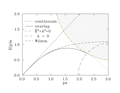
FIG. 9.: The dispersion relation for the overlap quark propagator of Eq. (A20) is shown as the solid line and corresponds to $\tilde{k}^{2}=0$. The dispersion relation does not continue into the region where $A>0$, i.e., it does not extend to the right beyond the long-dash dot line denoting $A=0$, [the solution of Eq. (A21)]. The analytic continuation to Minkowski space has no meaning when $\tilde{k}^{2}+A^{2}<0$, i.e., it is undefined above the short-dash dot line, [i.e., the solution of Eq. (A22)]. The intersection point of these three curves is where we simultaneously have $A$, $\tilde{k}^{2}$, and $\tilde{k}^{2}+A^{2}$ equal to zero. Also shown for reference are the dispersion relations for the continuum limit (short dashes) and for the ordinary Wilson action (long dashes).

REFERENCES

- [1] C.D. Roberts and A.G. Williams, Prog. Part. Nucl. Phys. 33, 477 (1994), [hep-ph/9403224].
- [2] F. D. R. Bonnet, P. O. Bowman, D. B. Leinweber, A. G. Williams and J. M. Zanotti, Phys. Rev. D 64, 034501 (2001) [hep-lat/0101013]; F. D. R. Bonnet, P. O. Bowman, D. B. Leinweber and A. G. Williams, Phys. Rev. D 62, 051501 (2000) [hep-lat/0002020]; D. B. Leinweber, J. I. Skullerud, A. G. Williams and C. Parrinello, Phys. Rev. D 60, 094507 (1999) [Erratum-ibid. D 61, 079901 (1999)] [hep-lat/9811027]; D. B. Leinweber, J. I. Skullerud, A. G. Williams and C. Parrinello Phys. Rev. D 58, 031501 (1998) [hep-lat/9803015].
- [3] D. Becirevic, V. Gimenez, V. Lubicz and G. Martinelli, Phys. Rev. D, 61, 114507 (2000) [hep-lat/9909082].
- [4] J. I. Skullerud and A. G. Williams, Phys. Rev. D 63, 054508 (2001) [hep-lat/0007028]; Nucl. Phys. Proc. Suppl. 83, 209 (2000) [hep-lat/9909142].
- [5] J. Skullerud, D. B. Leinweber and A. G. Williams, Phys. Rev. D 64, 074508 (2001) [hep-lat/0102013].
- [6] P. O. Bowman, U. M. Heller and A. G. Williams, Nucl. Phys. B (Proc. Suppl.) 106, 820 (2002); to appear in Nucl. Phys. Proc. Suppl., [hep-lat/0112027].
- [7] T. Blum et al., [hep-lat/0102005].
- [8] G. Martinelli, C. Pittori, C. T. Sachrajda, M. Testa and A. Vladikas, Nucl. Phys. B 445, 81 (1995) [arXiv:hep-lat/9411010].
- [9] M. Ciuchini, E. Franco, G. Martinelli, L. Reina and L. Silvestrini, Z. Phys. C 68, 239 (1995) [arXiv:hep-ph/9501265].
- [10] J. A. Skullerud, A. Kizilersu and A. G. Williams, to appear in Nucl. Phys. Proc. Suppl., [hep-lat/0109027].
- [11] N. Cabibbo and E. Marinari, Phys. Lett. B119, 387 (1982).
- [12] F. D. Bonnet, D. B. Leinweber and A. G. Williams, J. Comput. Phys. 170, 1 (2001) [hep-lat/0001017].
- [13] F. D. R. Bonnet, D. B. Leinweber, Anthony G. Williams and James M. Zanotti, “Symanzick improvement in the static quark potential”, [hep-lat/9912044].
- [14] A. Cucchieri and T. Mendes, Phys. Rev. D 57, 3822 (1998) [hep-lat/9711047].
- [15] F.D.R. Bonnet, P.O. Bowman, D.B. Leinweber, A.G. Williams and D.G. Richards, Austral J. Phys. 52, 939 (1999) [hep-lat/9905006].
- [16] R. Narayanan and H. Neuberger Nucl. Phys. B443, 305 (1995) [hep-th/9411108].
- [17] H. Neuberger, Phys. Rev. D 57, 5417 (1998) [hep-lat/9710089].
- [18] H. Neuberger, Phys. Lett. B427, 353 (1998) [hep-lat/9801031].
- [19] R. Narayanan and H. Neuberger, Nucl. Phys. B 443, 305 (1995) [hep-th/9411108].
- [20] F. Niedermayer, Nucl. Phys. Proc. Suppl. 73, 105 (1999) [hep-lat/9810026].
- [21] R.G. Edwards, U.M. Heller, and R. Narayanan, Phys. Rev. D 59, 094510 (1999) [hep-lat/9811030].
- [22] M. Luscher, Phys. Lett. B 428, 342 (1998) [hep-lat/9802011].
- [23] S. J. Dong, F. X. Lee, K. F. Liu and J. B. Zhang, Phys. Rev. Lett. 85, 5051 (2000) [hep-lat/0006004].
- [24] R. G. Edwards, U. M. Heller and R. Narayanan, Nucl. Phys. B540, 457 (1999) [hep-lat/9807017].
- [25] L. Giusti, C. Hoelbling, and C. Rebbi, Phys. Rev. D 64, 114508 (2001) [hep-lat/0108007]; L. Giusti, C. Hoelbling, C. Rebbi, Nucl. Phys. Proc. Suppl. 106, 739 (2002) [hep-lat/0110184].
- [26] R. G. Edwards, U. M. Heller and R. Narayanan, Nucl. Phys. B 535, 403 (1998) [hep-lat/9802016].
- [27] P. H. Ginsparg and K. G. Wilson Phys. Rev. D 25, 2649 (1982).
- [28] C. D. Roberts, [nucl-th/0007054]; Peter C. Tandy, in Proceedings of the Workshop on Lepton Scattering, Hadrons, and QCD, Adelaide, Australia, March-April 2001; [nucl-th/0106031]; P. Maris, C. D. Roberts and P. C. Tandy, Phys. Lett. B420, 267 (1998) [nucl-th/9707003].
- [29] R. Alkofer and L. von Smekal, Physics Reports 353, 281 (2001) [hep-ph/0007355].
- [30] A. Ringwald & F. Schrempp, Phys. Lett. B 459, 249 (1999) [hep-lat/9903039].
- [31] P. Hernandez, K. Jansen and L. Lellouch, Phys. Lett. B 469, 198 (1999) [hep-lat/9907022].
- [32] P. Hernandez, K. Jansen, L. Lellouch and H. Wittig, JHEP 0107, 018 (2001) [hep-lat/0106011].
- [33] T. DeGrand (MILC Collaboration), Phys. Rev. D 64, 117501 (2001) [hep-lat/0107014].
- [34] J. M. Zanotti et al. [CSSM Lattice Collaboration], [hep-lat/0110216].
- [35] W. Kamleh, D. Adams, D. B. Leinweber and A. G. Williams, [hep-lat/0112042] and [hep-lat/0112041].