Testing the self-duality of topological lumps in SU(3) lattice gauge theory

Abstract

We discuss a simple formula which connects the field-strength tensor to a spectral sum over certain quadratic forms of the eigenvectors of the lattice Dirac operator. We analyze these terms for the near zero-modes and find that they give rise to contributions which are essentially either self-dual or anti self-dual. Modes with larger eigenvalues in the bulk of the spectrum are more dominated by quantum fluctuations and are less (anti) self-dual. In the high temperature phase of QCD we find considerably reduced (anti) self-duality for the modes near the edge of the spectral gap.

Chiral symmetry breaking is one of the central pillars in our understanding of QCD. For the underlying mechanism an interesting picture based on instantons has been developed during the last 20 years [1]. The relevant excitations in the QCD vacuum are believed to consist of a weakly interacting fluid of instantons and anti-instantons. For a single instanton or anti-instanton the Dirac operator has an exact zero-mode. For the weakly interacting instantons and anti-instantons instead of many zero modes one expects the build-up of a non-vanishing density of small but non-zero eigenvalues corresponding to so-called near zero-modes. This spectral density near the origin is related to a non-vanishing chiral condensate through the Banks-Casher formula [2].

During the last year we have seen several papers [3]-[6] which test the scenario of chiral symmetry breaking through instantons with ab-initio calculations on the lattice, some supporting the instanton picture, some challenging it. The common basic idea is to study the properties of the near zero-modes of the lattice Dirac operator and to analyze whether one can identify localized structures which resemble instantons. The underlying assumption is that the near zero-modes are only slight deformations of zero-modes which in turn are known to be localized at the same position as the instanton.

In this letter we derive a simple formula which relates the field strength tensor $F_{\mu\nu}$ to a spectral sum over certain quadratic forms of the eigenvectors of the lattice Dirac operator. The terms in this spectral representation of the field strength, i.e. the quadratic forms of the eigenvectors, have a clear interpretation. One can analyze the contributions of the near zero-modes and test the scenario of chiral symmetry breaking through instantons.

In particular we will focus on analyzing the duality properties of the field strength. The possibility that the localized lumps in the field strength are not (anti) self-dual, i.e. do not have a fundamental property of (anti) instantons, has been brought up in Ref. [5], a paper which challenges the local quantization of topological charge in integer units. However, this possibility is ruled out by our current results: We find that the contributions to $F_{\mu\nu}$ which come from the near zero-modes do indeed show a high degree of (anti) self-duality. For contributions from eigenmodes with larger eigenvalues we find a decrease of (anti) self-duality as they are more dominated by quantum fluctuations.

When the temperature is increased beyond its critical value, QCD undergoes a phase transition where chiral symmetry is restored. In the instanton picture this transition is believed to be related to the formation of tightly bound instanton anti-instanton molecules. The spectrum develops a gap and due to the Banks-Casher formula the chiral condensate vanishes. When analyzing the modes with eigenvalues close to the edge of the spectral gap, we do indeed find a considerably reduced amount of (anti) self-duality as is expected for the tightly bound molecules.

We will denote the Dirac operator by $D=\gamma_{\mu}D_{\mu}$ with $D_{\mu}=\partial_{\mu}+A_{\mu}$. The gauge potential $A_{\mu}$ is anti-hermitian and in components is given by $A_{\mu}=-iA_{\mu}^{a}T_{a}$ where $T_{a},a=1..8$ are the generators of su(3). In this notation the field strength tensor is given by $F_{\mu\nu}=[D_{\mu},D_{\nu}]$, and in components reads $F_{\mu\nu}=-iF_{\mu\nu}^{a}T_{a}$. When evaluating the square of the Dirac operator one finds

$$D^{2}(x)\;=\;\sum_{\mu}D_{\mu}^{2}(x)+\sum_{\mu<\nu}\gamma_{\mu}\gamma_{\nu}F_{\mu\nu}(x)\;.$$ (1)

The field strength $F_{\mu\nu}$ can be projected out by multiplying $D^{2}$ with $\gamma_{\mu}\gamma_{\nu}$ and taking the trace over the Dirac indices. This results in the formula ($\mu\neq\nu$)

$$-\frac{1}{4}\mbox{Tr}_{D}\Big{[}\gamma_{\mu}\gamma_{\nu}D^{2}(x)\Big{]}\;=\;F_{\mu\nu}(x)\;,$$ (2)

for the field strength $F_{\mu\nu}$. For a lattice Dirac operator the situation is slightly more involved. On the lattice the Dirac operator is a difference operator and has two space-time indices $x,y$. When repeating the above calculation for e.g. Wilson’s lattice Dirac operator $D_{W}$, one finds (the indices $\mu,\nu$ on the right hand side are not summed)

$$- \frac{1}{4}\mbox{Tr}_{D}\Big{[}\gamma_{\mu}\gamma_{\nu}D^{2}_{W}(x,y)\Big{]}\;=\;F_{\mu\nu}(x)\;\frac{1}{4}[\delta_{x+\mu+\nu,y}$$ (3)

$$+ \delta_{x+\mu-\nu,y}+\delta_{x-\mu+\nu,y}+\delta_{x-\mu-\nu,y}]\;+\;{\cal O}(a^{2})\;.$$ (4)

Thus one finds that the field strength is slightly smeared out among several lattice points. We remark that an equivalent formula holds for staggered fermions where $\gamma_{\mu}\gamma_{\nu}$ is replaced by a staggered factor depending on $\mu,\nu$. For a general Dirac operator, such as the overlap operator [7], the fixed point operator [8] or the chirally improved operator [9] (which we use here) one finds (from now on we drop “${\cal O}(a^{2})$”)

$$F_{\mu\nu}(x)\;=\;-\frac{1}{4}\sum_{y}t_{y}(x)_{\mu\nu}\mbox{Tr}_{D}\Big{[}\gamma_{\mu}\gamma_{\nu}D^{2}(x,y)\Big{]}\;,$$ (5)

with some function $t_{y}(x)_{\mu\nu}$ which describes the smearing out of the field strength around the central point $x$. For the overlap operator this function is fast decaying in $|x-y|$ but has infinite support while for a finite approximation of the fixed point operator or the chirally improved operator $t_{y}(x)_{\mu\nu}$ will vanish for a sufficiently large separation of $x$ and $y$. One can show that a substantial contribution comes from $x=y$ and below we will concentrate on this particular case.

We now use the spectral representation of the Dirac operator to express the right hand side of Eq. (5) in terms of the eigenvectors $D(x,y)=\sum_{j}\lambda_{j}\;|j\rangle_{x}\;{}_{y}\langle j|$. In this formula we denote the eigenvectors by $|j\rangle_{x}$ and write explicitly only the space-time index $x$, while the color and Dirac indices are denoted with the bra-ket notation. The corresponding eigenvalues are denoted by $\lambda_{j}$. We remark that for non-normal operators, the bra’s ${}_{y}\langle j|$ have to be replaced by left eigenvectors and only the $|j\rangle_{x}$ are the conventional right eigenvectors [6].

After inserting the spectral decomposition of $D$ into our formula (5) we find:

$$F_{\mu\nu}^{a}(x) = \sum_{y}t_{y}(x)_{\mu\nu}\sum_{j}\lambda_{j}^{2}\;f^{a}_{\mu\nu}(x)_{y,j}\;,$$ (6)

$$f^{a}_{\mu\nu}(x)_{y,j} = -\frac{i}{2}\;{}_{y}\langle j|\gamma_{\mu}\gamma_{\nu}T_{a}|j\rangle_{x}\;.$$ (7)

In order to project onto the $a$-th component of the field strength tensor we have used $F_{\mu\nu}^{a}=i2$ Tr${}_{c}[F_{\mu\nu}T_{a}]$.

Equations (6) and (7) provide the announced spectral decomposition of the field strength tensor. One can now study the individual contributions $f^{a}_{\mu\nu}(x)_{y,j}$ in order to analyze properties of the field strength tensor. It is interesting to note that the exact zero modes do not contribute to the spectral decomposition (6),(7). Our formula has been tested on lattice discretizations of continuum instantons

Let us briefly comment on the setting of our numerical calculation. We study QCD in the quenched approximation using the Lüscher-Weisz action [10] with coefficients from tadpole improved perturbation theory. We work on lattices of size $16^{4}$ for the zero temperature ensembles and on $6\times 20^{3}$ lattices for the ensembles in the high temperature chirally symmetric phase. The leading coupling $\beta_{1}$ of the Lüscher-Weisz action is $\beta_{1}=8.45$ which corresponds to a lattice spacing of $a=0.095$ fm [11]. This value gives a temperature of 346 MeV for the high temperature ensemble. We use the chirally improved operator which is a systematic expansion of a solution of the Ginsparg-Wilson equation [9]. The computation of the eigenvalues and eigenvectors of the Dirac operator was done with the implicitly restarted Arnoldi method [12].

Let us begin our analysis of the terms in the spectral representation (6),(7) by displaying a single contribution $f^{a}_{\mu\nu}(x)_{y,j}$ and compare it to its dual $\widetilde{f^{a}_{\mu\nu}}(x)_{y,j}=1/2\;\varepsilon_{\mu\nu\rho\sigma}f^{a}_{\rho\sigma}(x)_{y,j}$. In particular in Fig. 1 we show a slice through the $16^{4}$ lattice and display the $f_{12}^{5}$ component in the top plot and the $f_{34}^{5}$ component in the bottom plot. We have set $x=y$, i.e. we show the center of the smeared-out field strength, and we evaluate the contribution for the first near zero-mode, i.e. the eigenvector with the smallest non-vanishing eigenvalue.

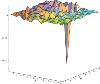
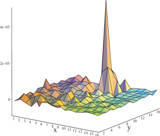
FIG. 1.: Contributions $f_{12}^{5}$ (top plot) and $f_{34}^{5}$ (bottom plot) of the first near zero-mode to the field strength. We show a slice of a $16^{4}$ lattice.

Both plots show a large peak accompanied by smaller wiggles. The peak changes sign but otherwise essentially keeps its size and shape when going from the $f_{12}^{5}$ to the $f_{34}^{5}$ component. Thus the peak is anti self-dual. For the smaller wiggles it is not straightforward to identify such a simple duality behavior - they are mainly quantum fluctuations. When inspecting many of these plots we find that the typical pattern consists of small quantum fluctuations and pronounced peaks which are either self-dual or anti self-dual. For contributions of eigenvectors with larger eigenvalues, so called bulk-modes, one finds that the abundance of isolated peaks decreases and the contributions become more dominated by quantum fluctuations.

Quantities of more physical interest are the action density Tr $F_{\mu\nu}F_{\mu\nu}$ and the topological charge density Tr $F_{\mu\nu}\widetilde{F_{\mu\nu}}$. In particular a direct comparison of the two quantities shows if the field is (anti) self-dual in all components. Again it is most interesting to analyze the contributions of the near zero-modes and see whether they are dominated by (anti) self-dual lumps as expected from the instanton picture. To this purpose we truncate the sum over the eigenvalues $\lambda_{i}$ in Eq. (6) and take into account only the first $N$ eigenvalues. In Fig. 2 we show

$$\mbox{Tr}\,F_{\mu\nu}(x)^{\prime}F_{\mu\nu}(x)^{\prime}=\sum_{i,j=1}^{N}\frac{\lambda_{i}^{2}\lambda_{j}^{2}}{2}f^{a}_{\mu\nu}(x)_{x,i}f^{a}_{\mu\nu}(x)_{x,j},$$ (8)

in the top plot. The color indices $a=1..8$ on the right hand side of (8) are summed to produce the color trace on the left hand side. The corresponding contribution to Tr $F_{\mu\nu}(x)^{\prime}\widetilde{F_{\mu\nu}}(x)^{\prime}$ is constructed in the same way and is displayed in the bottom plot of Fig. 2. For the figure we set $N=6$, i.e. we take into account only the contributions from the lowest 6 near zero-modes.

FIG. 2.: Tr $F_{\mu\nu}(x)^{\prime}F_{\mu\nu}(x)^{\prime}$ (top plot) and Tr $F_{\mu\nu}(x)^{\prime}$ $\widetilde{F_{\mu\nu}}(x)^{\prime}$ (bottom plot). The primes indicate the that we take into account only the contributions of the lowest 6 near zero-modes as defined in Eq.(8).

Both plots in Fig. 2 show two pronounced peaks with one of them changing sign when going from Tr $F_{\mu\nu}(x)^{\prime}F_{\mu\nu}(x)^{\prime}$ to Tr $F_{\mu\nu}(x)^{\prime}\widetilde{F_{\mu\nu}}(x)^{\prime}$. We remark that Figs. 1 and 2 were made from the same gauge configuration and the anti self-dual sign-changing peak of Fig. 2 is the same peak which we already saw in the contribution to the 5-component displayed in Fig. 1. The other smaller peak in Fig. 2 is a self-dual fluctuation in a different color component. Since the composed quantities Tr $F_{\mu\nu}(x)^{\prime}F_{\mu\nu}(x)^{\prime}$ and Tr $F_{\mu\nu}(x)^{\prime}\widetilde{F_{\mu\nu}}(x)^{\prime}$ are built from products of the single components $f_{\mu\nu}^{a}$ the relative size of the quantum fluctuations is suppressed considerably compared to the larger, (anti) self-dual structures. We find that the contributions of the near zero-modes to Tr $F_{\mu\nu}(x)^{\prime}F_{\mu\nu}(x)^{\prime}$ and Tr $F_{\mu\nu}(x)^{\prime}\widetilde{F_{\mu\nu}}(x)^{\prime}$ are entirely dominated by lumps which are either self-dual or anti self-dual.

In order to go beyond an illustration of the duality properties by a few examples we now discuss an observable which allows to test (anti) self-duality systematically. Its construction is similar to the chirality observable proposed in [4]. We define the ratio

$$r(x)\;=\;\frac{\mbox{Tr}\,F_{\mu\nu}(x)^{\prime}F_{\mu\nu}(x)^{\prime}\,-\,\mbox{Tr}\,F_{\mu\nu}(x)^{\prime}\widetilde{F_{\mu\nu}}(x)^{\prime}}{\mbox{Tr}\,F_{\mu\nu}(x)^{\prime}F_{\mu\nu}(x)^{\prime}\,+\,\mbox{Tr}\,F_{\mu\nu}(x)^{\prime}\widetilde{F_{\mu\nu}}(x)^{\prime}}\;.$$ (9)

For a space-time point $x$ where the gauge field is self-dual the numerator will vanish while the denominator is finite and $r(x)$ equals to 0. Conversely for an $x$ where the gauge field is anti self-dual the role of numerator and denominator are exchanged and $r(x)=\infty$. For space-time points without definite duality properties $r(x)$ assumes some finite value between 0 and $\infty$. The transformation $R(x)=4/\pi\arctan r(x)-1$ maps the interval $[0,\infty)$ into the interval $[-1,1]$. For configurations which are dominated by (anti) self-dual lumps one expects values near $\pm 1$. As for the local chirality variable of [4] it is interesting to study different selections for the lattice points $x$ in $R(x)$. In Fig. 3 we use all lattice points (top curve), the subset of 50% of the lattice points supporting the highest peaks of $|$Tr $F_{\mu\nu}(x)^{\prime}\widetilde{F_{\mu\nu}(x)^{\prime}}|$ (middle curve) and also a cut of 10% (bottom curve). Again we use the 6 lowest modes in the series for $F_{\mu\nu}(x)^{\prime}$. The histograms were computed by averaging over 50 configurations.

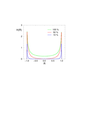
FIG. 3.: Histograms for the observable $R$ which tests the (anti) self-duality of the near zero-modes (compare Eq. (9)). We display our data without a cut (top curve), a cut of 50% (middle curve) and a cut of 10 % on the number of lattice points supporting the highest peaks of $|$Tr$F_{\mu\nu}(x)^{\prime}\widetilde{F_{\mu\nu}}(x)^{\prime}|$.

Fig. 3 shows that the contributions of the near zero-modes to the spectral representation of the field strength are highly (anti) self-dual. Even when including all lattice points (100%, top curve) one finds a pronounced double peak. When throwing away 50% of the lattice points with small $|$Tr$F_{\mu\nu}(x)^{\prime}\widetilde{F_{\mu\nu}}(x)^{\prime}|$ this cuts mainly into the center of the histogram, showing that the most (anti) self-dual excitations are indeed the large peaks sticking out of the quantum fluctuations. This trend continues when focusing on only the highest 10% of the peaks. Since our analysis is based on the exact spectral decomposition of the field strength it truly reflects self-duality of the topological lumps in the gauge field.

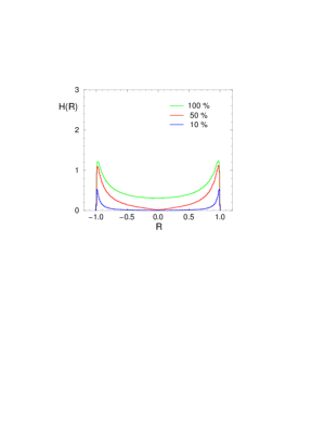
FIG. 4.: The same as in Fig. 3 but now for the ensemble in the chirally symmetric phase of QCD.

It is interesting to perform the same analysis also in the chirally symmetric phase of QCD. As discussed, the instanton picture describes this phase by tightly bound molecules of instantons and anti-instantons [1]. In Fig. 4 we show our results for the histograms of the duality observable $R$ for our ensembles in the high temperature phase. Again we average over 50 configurations. $F_{\mu\nu}(x)^{\prime}$ is now computed from the 6 modes with eigenvalues closest to the edge of the spectral gap. Obviously the amount of (anti) self-duality has decreased considerably which is exactly what is expected to happen when instantons and anti-instantons condense to tightly bound molecules and lose their identity as isolated (anti) self-dual objects.

Let us briefly summarize the obtained results. We derive a representation of the field strength in terms of a spectral sum of quadratic forms of the eigenvectors of the lattice Dirac operator. The contributions of individual eigenvectors to the field strength can be analyzed. We find that the near zero-modes are dominated by (anti) self-dual lumps, while modes with larger eigenvalues further in the bulk of the spectrum become dominated by quantum fluctuations. Our spectral representation thus decomposes the field strength tensor into contributions (the near zero-modes) sensitive to the large scale fluctuations and contributions (the bulk modes) dominated by quantum fluctuations. In the high temperature phase we find a reduced amount of (anti) self-duality for the modes with eigenvalues near the edge of the spectral gap. Our results support the picture of chiral symmetry breaking by instantons and its restoration through the formation of instanton anti-instanton molecules. Acknowldegements: I would like to thank Pierre van Baal, Tom DeGrand, Meinulf Göckeler, Ivan Hip, Christian Lang, Paul Rakow, Stefan Schaefer and Andreas Schäfer for discussions and the Austrian Academy of Science for support (APART 654). The calculations were done on the Hitachi SR8000 at the Leibniz Rechenzentrum in Munich and I thank the LRZ staff for training and support.

REFERENCES

- [1] D. Diakonov and V.Y. Petrov, Phys. Lett. B 147 (1984) 351; Nucl. Phys. B 272 (1986) 457; D. Diakonov, Talk given at International School of Physics, ’Enrico Fermi’, Course 80: Selected Topics in Nonperturbative QCD, Varenna, Italy, 1995, hep-ph/9602375; T. Schäfer and E.V. Shuryak, Rev. Mod. Phys. 70 (1998) 323.
- [2] T. Banks and A. Casher, Nucl. Phys. B169 (1980) 103.
- [3] T.L. Ivanenko and J. W. Negele, Nucl. Phys. Proc. Suppl. 63 (1998) 504; T. DeGrand and A. Hasenfratz, Phys. Rev. D 64 (2001) 034512; M. Göckeler, P.E.L. Rakow, A. Schäfer, W. Söldner, T. Wettig, Phys. Rev. Lett. 87 (2001) 042001; T. DeGrand, Phys. Rev. D 64 (2001) 094508; C. Gattringer, M. Göckeler, P.E.L. Rakow, S. Schaefer, A. Schäfer, Nucl. Phys. B 617 (2001) 101; Nucl. Phys. B 618 (2001) 205; C. Gattringer, M. Göckeler, C. B. Lang, P.E.L. Rakow, A. Schäfer, Phys. Lett. B 522 (2001) 194; T. DeGrand and A. Hasenfratz, Phys. Rev. D 65 (2002) 014503; T. Blum et al., Phys. Rev. D 65 (2002) 014504; R. G. Edwards and U. M. Heller, Phys. Rev. D 65 (2002) 014505; P. Hasenfratz, S. Hauswirth, K. Holland, T. Jörg and F. Niedermayer, Nucl. Phys. Proc. Suppl. 106 (2002) 751.
- [4] I. Horváth, N. Isgur, J. McCune and H. B. Thacker, Phys. Rev. D 65 (2002) 014502.
- [5] I. Horváth et al., hep-lat/0201008.
- [6] I. Hip, T. Lippert, H. Neff, K. Schilling and W. Schroers, Phys. Rev. D 65 (2002) 014506.
- [7] R. Narayanan and H. Neuberger, Phys. Lett. B 302 (1993) 62, Nucl. Phys. B 443 (1995) 305.
- [8] P. Hasenfratz, Nucl. Phys. B (Proc. Suppl.) 63 (1998) 53; P. Hasenfratz, Nucl. Phys. B 525 (1998) 401; P. Hasenfratz, S. Hauswirth, K. Holland, Th. Jörg, F. Niedermayer, U. Wenger, Int. J. Mod. Phys. C 12 (2001) 691.
- [9] C. Gattringer, Phys. Rev. D 63 (2001) 114501; C. Gattringer, I. Hip, C.B. Lang, Nucl. Phys. B597 (2001) 451.
- [10] M. Lüscher and P. Weisz, Commun. Math. Phys. 97 (1985) 59; Err.: 98 (1985) 433; G. Curci, P. Menotti and G. Paffuti, Phys. Lett. B 130 (1983) 205, Err.: B 135 (1984) 516; M. Alford, W. Dimm, G.P. Lepage, G. Hockney and P.B. Mackenzie, Phys. Lett. B 361 (1995) 87.
- [11] C. Gattringer, R. Hoffmann,S . Schaefer, hep-lat/ 0112024, Phys. Rev. D in print.
- [12] D.C. Sorensen, SIAM J.Matrix Anal.Appl.13 (1992) 357.