UTHEP-454 UTCCP-P-120 December 2001 Charmonium Spectrum from Quenched Anisotropic Lattice QCD

Abstract

We present a detailed study of the charmonium spectrum using anisotropic lattice QCD. We first derive a tree-level improved clover quark action on the anisotropic lattice for arbitrary quark mass by matching the Hamiltonian on the lattice and in the continuum. The heavy quark mass dependence of the improvement coefficients, i.e. the ratio of the hopping parameters $\zeta=K_{t}/K_{s}$ and the clover coefficients $c_{s,t}$, are examined at the tree level, and effects of the choice of the spatial Wilson parameter $r_{s}$ are discussed. We then compute the charmonium spectrum in the quenched approximation employing $\xi=a_{s}/a_{t}=3$ anisotropic lattices. Simulations are made with the standard anisotropic gauge action and the anisotropic clover quark action with $r_{s}=1$ at four lattice spacings in the range $a_{s}$=0.07-0.2 fm. The clover coefficients $c_{s,t}$ are estimated from tree-level tadpole improvement. On the other hand, for the ratio of the hopping parameters $\zeta$, we adopt both the tree-level tadpole-improved value and a non-perturbative one. The latter employs the condition that the speed of light calculated from the meson energy-momentum relation be unity. We calculate the spectrum of S- and P-states and their excitations using both the pole and kinetic masses.

We find that the combination of the pole mass and the tadpole-improved value of $\zeta$ to yield the smoothest approach to the continuum limit, which we then adopt for the continuum extrapolation of the spectrum. The results largely depend on the scale input even in the continuum limit, showing a quenching effect. When the lattice spacing is determined from the $1P-1S$ splitting, the deviation from the experimental value is estimated to be $\sim$30% for the S-state hyperfine splitting and $\sim$20% for the P-state fine structure. Our results are consistent with previous results at $\xi=2$ obtained by Chen when the lattice spacing is determined from the Sommer scale $r_{0}$.

We also address the problem with the hyperfine splitting that different choices of the clover coefficients lead to disagreeing results in the continuum limit. Making a leading order analysis based on potential models we show that a large hyperfine splitting $\sim$95 MeV obtained by Klassen with a different choice of the clover coefficients is likely an overestimate.

I Introduction

Lattice study of heavy quark physics is indispensable for determining the standard model parameters such as the quark masses and CKM matrix elements, and for finding signals of new physics beyond it. Obtaining accurate results for heavy quark observables, however, is a non-trivial task. Since lattice spacings of order $a\approx(2\mbox{GeV})^{-1}$ currently accessible is comparable or even larger than the Compton wavelength of heavy quark given by $1/m_{q}$ for charm and bottom, a naive lattice calculation with conventional fermion actions suffers from large uncontrolled systematic errors. For this reason, effective theory approaches for heavy quark have been pursued.

One of the approaches is the lattice version of the non-relativistic QCD (NRQCD), which is applicable for $a>1/m_{q}$ [1, 2]. Since the expansion parameter of NRQCD is the quark velocity squared $v^{2}$, lattice NRQCD works well for sufficiently heavy quark such as the the bottom ($v^{2}\sim 0.1$), and the bottomonium spectrum [3, 4, 5, 6] and the $b\bar{b}g$ hybrid spectrum [7, 8, 9, 10] have been studied successfully using lattice NRQCD. An serious constraint with the approach, however, is that the continuum limit cannot be taken due to the condition $a>1/m_{q}$. Thus scaling violation from the gauge and light quark sectors should be sufficiently small. In practice it is often difficult to quantify the magnitude of systematic errors arising from this origin. Another difficulty is that there are a number of parameters in the NRQCD action which have to be determined. Since in the present calculations the tuning of parameters is made at the tree level (or tadpole improved tree level) of perturbation theory, the accuracy achieved is rather limited.

Another approach for heavy quark uses a space-time asymmetric quark action, aiming to implement the $O(a)$ improvement for arbitrary quark mass [11]. With appropriate parameter tunings, this action is unitarily equivalent to the NRQCD action up to higher order corrections for $a>1/m_{q}$, and goes over into the light quark Sheikholeslami-Wohlert (SW) action [12] for $am_{q}\ll 1$. This approach has been originally proposed by the Fermilab group and the action is hence called the “Fermilab action”, whose first application is found in [13]. Since the necessary tuning of mass-dependent parameters is in general difficult, in practice one uses the usual SW quark action even for $a>1/m_{q}$, where the SW action is unitarily equivalent to NRQCD. This simplified approach, called the “non-relativistic interpretation” for the SW quark, has been widely used in current lattice simulations of heavy quark, such as the calculation of the $B$ meson decay constant [14, 15, 16, 17]. Toward the continuum limit $a\to 0$ the lattice action approaches the usual $O(a)$-improved action and the systematic error becomes smaller as $(am_{q})^{2}$. However, the $am_{q}$ dependence at $am_{q}\raise 1.29167pt\hbox{$>$\kern-7.5pt\raise-4.73611pt\hbox{$\sim$}}1$ is quite non-linear, and it is not trivial how the systematic error could be controlled.

Recently use of the anisotropic lattice for heavy quark simulations has been proposed [18, 19] as a possible alternative to solve the difficulties of the effective approach. On an anisotropic lattice, where the temporal lattice spacing $a_{t}$ is smaller than the spatial one $a_{s}$, one can achieve $a_{t}m_{q}\ll 1$ while keeping $a_{s}m_{q}\sim 1$. Therefore, using anisotropic lattices, one can reduce $O((a_{t}m_{q})^{n})$ ($n=1,2,\cdots$) discretization errors while the computer cost is much less than that needed for the isotropic lattice at the same $a_{t}$. Naively it is expected that the reduction of $O((a_{t}m_{q})^{n})$ errors entails the reduction of most of discretization errors due to large quark mass, since the on-shell condition ensures that the large energy scale flows only into the temporal direction as far as one considers the static particle, with zero or small spatial momentum. If such a naive expectation is correct, the discretization error is controlled by a small parameter $a_{t}m_{q}$ as it is for light quarks, and one can achieve even better accuracy by taking a continuum limit. However, it is not obvious that one can eliminate all $O((a_{s}m_{q})^{n})$ errors at the quantum level, even if it is possible at the tree level.

Another advantage of the anisotropic lattice, which is more practical, is that a finer temporal resolution allows us to determine large masses more accurately. This has been already demonstrated in simulations of the glueball [20, 21] and the hybrid meson [8].

Klassen calculated the charmonium spectrum in the quenched approximation, employing lattices with the ratio of the temporal and spatial lattice spacings $\xi\equiv a_{s}/a_{t}=2$ and 3, as a feasibility study of the anisotropic approach [18, 19]. He tuned the ratio of the temporal and spatial hopping parameters $\zeta\equiv K_{t}/K_{s}$ non-perturbatively by demanding the relativistic dispersion relation for mesons. For the spatial clover coefficient $c_{s}$, he adopted two choices, the tree level tadpole improved value correct for any mass ($a_{t}m_{q}\geq 0$) and that correct only in the massless ($a_{t}m_{q}=0$) limit, in order to make a comparison. He mainly studied the spin splitting of the spectrum, and obtained an unexpected result that two different choices of the clover coefficients lead to two different values of the S-state hyperfine splitting even in the continuum limit [18, 19]. The continuum limit is of course unique, and clearly, at least one of the two continuum extrapolations is misleading. Since the hyperfine splitting is sensitive to the clover coefficients, it is plausible that the disagreement is due to a large discretization error arising from the choice of the clover coefficients. In an unpublished paper [19], he pointed out the possibility that the $O((\xi a_{t}m_{q})^{n})=O((a_{s}m_{q})^{n})$ errors still remain with his choice of the parameters, which we review in the next section. A similar statement can be found in some recent studies [22, 23]. In fact, he adopted rather coarse lattice spacings $a_{s}\simeq 0.17-$0.30 fm where $a_{s}m_{q}\sim 1$. It is then questionable whether the reliable continuum extrapolation is performed at such coarse lattice spacings.

Using the same anisotropic approach as Klassen, Chen has recently calculated the quenched charmonium spectrum [24]. She employed $\xi=2$ and finer ($a_{s}\simeq 0.10-$0.25 fm) lattices, and adopted the tree level tadpole improved clover coefficient $c_{s}$ correct for any mass, which is expected to be better than the other choice that is correct only in the massless limit. She computed not only the ground state masses but also the first excited state masses, and extrapolated them to the continuum limit. Her results at $\xi=2$ are consistent with Klassen’s results at $\xi=2$ and 3 with the same choice of the clover coefficients.

Since Chen’s calculation was performed only at $\xi=2$, similar calculations at different values of $\xi$ using fine lattices are needed to check the reliability of the continuum limit from the anisotropic approach. In addition, the complete P-state fine structure has not yet obtained in this approach so far, since the mass of ${}^{3}P_{2}(\chi_{c2})$ state has not been measured in previous studies.

In this work, we present a detailed study of the charmonium spectrum from the anisotropic lattice QCD. We perform simulations in the quenched approximation at $\xi=3$, employing fine lattice spacings in the range $a_{s}=0.07-$0.2 fm. We attempt to determine the ground state masses of all the S- and P-states (including ${}^{3}P_{2}$) as well as their first excited state masses. To estimate the systematic errors accurately, we adopt both the tree level tadpole improved value and non-perturbative one for $\zeta$, and both the pole mass and kinetic mass for $M_{\rm lat}(1\bar{S})$ which is tuned to the experimental value. We focus on the lattice spacing dependence and continuum limit of the mass splittings. We compare our results with the previous anisotropic results by Klassen and Chen to check the consistency, and with experimental values [25] to estimate the quenching effect.

In addition, to understand the discrepancy of the hyperfine splitting mentioned above, we make a leading order analysis using the potential model. To examine the effect of clover coefficients, we estimate the hyperfine splitting at leading order. Comparing the leading order estimates with numerical results for the hyperfine splitting, we attempt to find a probable solution for this problem. Our preliminary results are already reported in Refs. [26, 27].

This paper is organized as follows. In Section II, we summarize and discuss the theoretical aspect of the anisotropic lattice QCD. In Section III, we give details of our simulation. Our results for the charmonium spectra are shown in Section IV, where we attempt to take the continuum limit and estimate the quenching effect. We address the problem of the discrepancy of the hyperfine splitting and study the effect of clover coefficients in Section V. Section VI is devoted to our conclusions.

II Anisotropic lattice QCD action

In this section we first define the anisotropic lattice action used in this work and fix notations. We then derive the tree level values of bare parameters in our massive quark action, and discuss effects of the anisotropy. Although it was already discussed in earlier papers [22, 23], we briefly describe the outline of derivations in order to be self-contained. We also consider the tadpole improvement of bare parameters and see how tree level values are modified.

A Anisotropic gauge action

In this work, we use the standard Wilson gauge action defined on an anisotropic lattice:

$$S_{g}=\beta\left[\frac{1}{\xi_{0}}\sum_{x,s>s^{\prime}}(1-P_{ss^{\prime}}(x))+\xi_{0}\sum_{x,s}(1-P_{st}(x))\right]$$ (1)

where $\beta=6/g^{2}$ is the gauge coupling, and $P_{ss^{\prime}}(x)$ and $P_{st}(x)$ are the spatial and temporal plaquettes with $P_{\mu\nu}(x)=\frac{1}{3}\mbox{Re}\ \mbox{Tr}\ U_{\mu\nu}(x)$. The anisotropy is introduced by the parameter $\xi_{0}$ and we call this the “bare anisotropy”. We denote spatial and temporal lattice spacings as $a_{s}$ and $a_{t}$ and define the “renormalized anisotropy” $\xi\equiv a_{s}/a_{t}$. We have $\xi=\xi_{0}$ at the tree level, and the $\xi=\xi(\xi_{0},\beta)$ at finite $\beta$ can be determined non-perturbatively by Wilson loop matching [28, 29, 30]. In numerical simulations, there are two methods for anisotropy tuning, either varying $\xi_{0}$ to keep $\xi$ constant or vice versa. Since the former is more convenient for keeping the physical size constant, and easier for performing the continuum extrapolation, we adopt it in this work.

B Anisotropic quark action

For the quark action, we employ the space-time asymmetric clover quark action on an anisotropic lattice proposed in Ref. [18, 19]:

$$S_{f} = \sum_{x}\bar{\psi}_{x}Q\psi_{x},$$ (2)

$$Q = m_{0}+\nu_{0}\hat{W}_{0}\gamma_{0}+\frac{\nu}{\xi_{0}}\sum_{i}\hat{W}_{i}\gamma_{i}+\frac{i}{2}\left[\omega_{0}\sum_{x,i}\sigma_{0i}\hat{F}_{0i}(x)+\frac{\omega}{\xi_{0}}\sum_{x,i<j}\sigma_{ij}\hat{F}_{ij}(x)\right],$$ (3)

where $\nu_{0}=1$ and $m_{0}\equiv a_{t}m_{q0}$ is the bare quark mass, and $\hat{W}_{\mu}\gamma_{\mu}\equiv a_{\mu}W_{\mu}\gamma_{\mu}$ and $\hat{F}_{\mu\nu}\equiv a_{\mu}a_{\nu}F_{\mu\nu}$ with $(a_{0},a_{i})=(a_{t},a_{s})$. The Wilson operator $W_{\mu}$ is defined by

$$W_{\mu}\gamma_{\mu}\equiv D_{\mu}\gamma_{\mu}-\frac{a_{\mu}}{2}r_{\mu}D^{2}_{\mu}\;\;\;\;(\mu=0,1,2,3)$$ (4)

with the Wilson coefficients $(r_{0},r_{i})=(r_{t},r_{s})$ and

$$D_{\mu}\psi_{x} \equiv \frac{1}{2a_{\mu}}\left[U_{\mu,x}\psi_{x+\hat{\mu}}-U^{\dagger}_{\mu,x-\hat{\mu}}\psi_{x-\hat{\mu}}\right],$$ (5)

$$D^{2}_{\mu}\psi_{x} \equiv \frac{1}{a_{\mu}^{2}}\left[U_{\mu,x}\psi_{x+\hat{\mu}}+U^{\dagger}_{\mu,x-\hat{\mu}}\psi_{x-\hat{\mu}}-2\psi_{x}\right].$$ (6)

For the field tensor $F_{\mu\nu}$, we adopt the standard clover leaf definition. Note that, in Eq. (3), the factors in front of spatial Wilson and clover operators include $\xi_{0}$ rather than $\xi$. This is merely a convention and there is no deep theoretical reason. This action is essentially the same as the one employed by Klassen[19] and Chen[24]. In Chen’s work, however, $\nu_{0}$ was a tuning parameter with $\nu=1$ fixed. The two parameterizations are related to each other by a field rescaling $\psi_{x}\rightleftharpoons\psi_{x}/\sqrt{\nu}$. Therefore $\{m_{0},\nu_{0},\omega,\omega_{0}\}$ corresponds to $\{m_{0}/\nu,1/\nu,\omega/\nu,\omega_{0}/\nu\}$ in our convention. Among these six parameters $\{m_{0},\nu,r_{s},r_{t},\omega,\omega_{0}\}$, at least one is redundant, so that we take $r_{t}$ as a redundant parameter and use it to remove the fermion doublers. Although $r_{s}$ may not be taken arbitrary in the $O(a)$ improved anisotropic quark action [23] for the matrix elements, it can be taken arbitrary for the hadron mass calculation. Therefore we always set $r_{t}=1$ and leave $r_{s}$ free in this work. The remaining parameters $\{m_{0},\nu,\omega,\omega_{0}\}$ are used to tune the quark mass and reduce the lattice discretization error.

For convenience in numerical simulations, we also present the quark action in a different form. Rescaling the fields $\psi_{x}$, the quark action can be transformed into a form given by

$$S_{f}^{\prime}=\sum_{x}\{\bar{\psi}_{x}\psi_{x} - K_{t}[\bar{\psi}_{x}(1-\gamma_{0})U_{0,x}\psi_{x+\hat{0}}+\bar{\psi}_{x}(1+\gamma_{0})U^{\dagger}_{0,x-\hat{0}}\psi_{x-\hat{0}}]$$ (7)

$$- K_{s}\sum_{i}[\bar{\psi}_{x}(r_{s}-\gamma_{i})U_{i,x}\psi_{x+\hat{i}}+\bar{\psi}_{x}(r_{s}+\gamma_{i})U^{\dagger}_{i,x-\hat{i}}\psi_{x-\hat{i}}]\}$$ (8)

$$+ iK_{s}c_{s}\sum_{x,i<j}\bar{\psi}_{x}\sigma_{ij}\hat{F}_{ij}(x)\psi_{x}+iK_{s}c_{t}\sum_{x,i}\bar{\psi}_{x}\sigma_{0i}\hat{F}_{0i}(x)\psi_{x},$$ (9)

where $K_{s,t}$ and $c_{s,t}$ are the spatial and temporal hopping parameters and the clover coefficients, respectively. The hopping parameters $K_{s,t}$ are related to the bare quark mass $m_{0}=a_{t}m_{q0}$ through

$$a_{t}m_{q0}\equiv 1/(2K_{t})-3r_{s}/\zeta-1,\;\;\;\;\;\;\zeta\equiv K_{t}/K_{s}.$$ (10)

The form Eq. (9) on the anisotropic lattice is the same as that on the isotropic lattice in Ref. [11]. Note however that Ref. [11] uses the inverse of our definition for $\zeta$. We refer to their definition as $\zeta_{\rm F}\equiv K_{s}/K_{t}=1/\zeta$. Using Eq. (10) one can convert $\{m_{q0},\zeta\}$ to $\{K_{s},K_{t}\}$. In our convention, the relation between $\{\nu,\omega,\omega_{0}\}$ and $\{\zeta,c_{s},c_{t}\}$ is given by

$$\zeta=\xi_{0}/\nu,\;\;\;c_{s}=\omega/\nu,\;\;\;c_{t}=\xi_{0}\omega_{0}/\nu$$ (11)

or equivalently,

$$\nu=\xi_{0}/\zeta,\;\;\;\omega=c_{s}\nu,\;\;\;\omega_{0}=c_{t}\nu/\xi_{0}.$$ (12)

Following Ref. [11], we call the quark action Eq. (3) as the “mass form” and Eq. (9) as the “hopping parameter form”.

C Tree level tuning of bare parameters for arbitrary mass

To derive the tree level value of bare parameters, we follow the Fermilab method and calculate the lattice Hamiltonian[11]. After some algebra (see appendix A for details), we obtain the lattice Hamiltonian Eq. (A9). Using the FWT transformation Eq. (A17), we then transform it to the non-relativistic form, in which the upper components of the Dirac spinor completely decouple from the lower ones (i.e. eliminate ${\bf\gamma}\cdot{\bf D}$ and ${\bf\alpha}\cdot{\bf E}$). The transformed Hamiltonian is given by

$$\frac{1}{a_{t}}\hat{H}^{U}=\hat{\bar{\Psi}}\left(m_{1}+\gamma_{0}A_{0}-\frac{{\bf D}^{2}}{2m_{2}}-\frac{i{\bf\Sigma}\cdot{\bf B}}{2m_{B}}-\gamma_{0}\frac{[{\bf\gamma}\cdot{\bf D},{\bf\gamma}\cdot{\bf E}]}{8m_{E}^{2}}+\cdots\right)\hat{\Psi}$$ (13)

with

$$a_{t}m_{1} = \log(1+m_{0}),$$ (14)

$$\frac{1}{a_{t}m_{2}} = \frac{2{\zeta_{\rm F}^{\prime}}^{2}}{m_{0}(2+m_{0})}+\frac{r_{s}^{\prime}\zeta_{\rm F}^{\prime}}{1+m_{0}},$$ (15)

$$\frac{1}{a_{t}m_{B}} = \frac{2{\zeta_{\rm F}^{\prime}}^{2}}{m_{0}(2+m_{0})}+\frac{c_{s}^{\prime}\zeta_{\rm F}^{\prime}}{1+m_{0}},$$ (16)

$$\frac{1}{(a_{t}m_{E})^{2}} = 4{\zeta_{\rm F}^{\prime}}^{2}\left[\frac{(1+m_{0})^{2}}{m_{0}^{2}(2+m_{0})^{2}}+(c_{t}-1)\frac{1}{m_{0}(2+m_{0})}\right],$$ (17)

where $\zeta_{\rm F}^{\prime}$, $r_{s}^{\prime}$ and $c_{s}^{\prime}$ are defined in Eq. (A8). The ${\bf\Sigma}\cdot{\bf B}$ term gives the leading order contribution to the hyperfine splitting, while $[{\bf\gamma}\cdot{\bf D},{\bf\gamma}\cdot{\bf E}]$ term yields the fine structure splitting.

The matching condition $\hat{H}^{U}=\hat{H}_{\rm NR}+O(a_{s}^{2})$ is equivalent to

$$m_{1}=m_{2}=m_{B}=m_{E}=m_{q}.$$ (18)

This yields the tree level value of bare parameters for massive quark:

$$\xi_{0}\zeta_{\rm F}=\nu=\sqrt{\left(\frac{\xi_{0}r_{s}m_{0}(2+m_{0})}{4(1+m_{0})}\right)^{2}+\frac{m_{0}(2+m_{0})}{2\log(1+m_{0})}}-\frac{\xi_{0}r_{s}m_{0}(2+m_{0})}{4(1+m_{0})},$$ (19)

$$c_{s}=r_{s}\,\,\,\,\,\,(\omega=r_{s}\nu),$$ (20)

$$c_{t}=\frac{(\xi_{0}\zeta_{\rm F})^{2}-1}{m_{0}(2+m_{0})}+\frac{\xi_{0}^{2}r_{s}\zeta_{\rm F}}{1+m_{0}}+\frac{(\xi_{0}r_{s})^{2}m_{0}(2+m_{0})}{4(1+m_{0})^{2}}.$$ (21)

We note that $c_{s}$ is independent of the quark mass, while $\nu$ and $c_{t}$ have complicated mass dependences. The term $\xi_{0}m_{0}\simeq a_{s}m_{q0}$ seems to exist in Eq. (19) and (21). To see this explicitly, we expand $\nu$ and $c_{t}$ in $m_{0}$. This gives

$$\nu=1+\frac{1}{2}(1-\xi_{0}r_{s})m_{0}+\frac{1}{24}(-1+6\xi_{0}r_{s}+3(\xi_{0}r_{s})^{2})m_{0}^{2}+O(m_{0}^{3}),$$ (22)

$$c_{t}=\frac{1+\xi_{0}r_{s}}{2}+\frac{1}{12}(-2-3\xi_{0}r_{s}+3(\xi_{0}r_{s})^{2})m_{0}+O(m_{0}^{2}).$$ (23)

The $a_{s}m_{q0}$ term, which is $O(1)$ for heavy quarks at currently accessible lattice spacings of $a_{s}^{-1}\approx 2$ GeV, appears in $\nu$ and $c_{t}$ even at the tree level. Since $\xi_{0}m_{0}=a_{s}m_{q0}$ is always multiplied with the spatial Wilson coefficient $r_{s}$ in Eqs. (22) and (23), one can eliminate the $a_{s}m_{q0}$ term at the tree level by choosing

$$r_{s}=1/\xi_{0}.$$ (24)

However, this choice has the disadvantage that the mass splitting between unphysical doubler states and the physical state decreases as $\xi_{0}$ increases. Moreover, the hopping terms in the quark action are no longer proportional to the $1\pm\gamma_{\mu}$ projection operators. It is also doubtful that, beyond the tree level, the $a_{s}m_{q0}$ term can be still eliminated by this choice.

If one adopts the conventional choice

$$r_{s}=1,$$ (25)

the $a_{s}m_{q0}$ term remains, but the unphysical doubler states decouple. This choice also has the practical merit that the quark action has the full projection property, so that the coding is easier and the computational cost is lower.

The tree-level full mass dependences of $\nu$ and $c_{t}$ for $r_{s}=1/\xi_{0}$ and $r_{s}=1$ are shown in Figs. 1 and 2. In order to compare at the same $a_{s}$, we choose $m_{1}a_{s}$ as the horizontal axis instead of $m_{1}a_{t}$ where $m_{1}$ is the pole mass. Since $a_{s}^{-1}\raise 1.29167pt\hbox{$>$\kern-7.5pt\raise-4.73611pt\hbox{$\sim$}}1$ GeV and $m_{1}\leq m_{\rm bottom}\sim 4.5$ GeV in current typical simulations, we plot results for $m_{1}a_{s}\leq 4$.

For $r_{s}=1/\xi_{0}$ shown in Fig. 1, both $\nu$ and $c_{t}$ are monotonic functions in mass, and they converge to their massless values as $\xi_{0}$ increases at any fixed values of $m_{1}a_{s}$. Hence, the $a_{s}m_{q0}$ dependence can be controlled by increasing $\xi_{0}$. At $\xi=100$ the mass dependences of $\nu$ and $c_{t}$ completely disappear with the cost that the physical and unphysical states are almost degenerate. In actual simulations with $r_{s}=1/\xi_{0}$, taking $2\leq\xi_{0}\ll\infty$ to decouple unphysical doublers, one is allowed to use the massless values for $\nu$ and $c_{t}$, since their mass dependences are monotonic and very weak. In this case mass dependent parameter tuning can be avoided even at $a_{s}m_{0}\sim 1$.

For $r_{s}=1$, on the other hand, the mass dependences of $\nu$ and $c_{t}$ are complicated and non-negligible even for large $\xi_{0}$. Indeed $\nu$ and $c_{t}$ do not converge to their massless values as $\xi_{0}$ increases at fixed $m_{1}a_{s}$, as shown in Fig. 2. The deviation from the massless values at $\xi_{0}=2$ is smaller than the one at $\xi_{0}=1$, but it becomes larger again as $\xi_{0}$ increases. Therefore, taking $\xi_{0}=2$-3 in simulations with $r_{s}=1$, one needs to perform a mass dependent parameter tuning.

For both choices of $r_{s}$, it is better to use a moderate value of $\xi_{0}$, rather than excessively large values. In our numerical study of the charmonium spectra, we adopt the choice $r_{s}=1$, and make a mass dependent parameter tuning, due to the practical reasons mentioned above.

Finally we show the tree level value of the parameters in the massless limit. By taking $a_{t}m_{q0}\rightarrow 0$ in Eqs. (19)-(21), one obtains

$$\nu=1,\;\;\;\omega=r_{s},\;\;\;\omega_{0}=\frac{1+\xi_{0}r_{s}}{2\xi_{0}},$$ (26)

in the mass form, or

$$\zeta=\xi_{0},\;\;\;c_{s}=r_{s},\;\;\;c_{t}=\frac{1+\xi_{0}r_{s}}{2}.$$ (27)

in the hopping parameter form. Note that there is an ambiguity in the tree level value of $a_{s}/a_{t}$, since $\xi_{0}=\xi$ at the tree level but $\xi_{0}\not=\xi$ in the simulation. Fortunately, this ambiguity almost disappears after the tadpole improvement, as shown in the next subsection.

D Tadpole improvement

In this section we apply the tadpole improvement [31] to the parameters of the anisotropic lattice action at tree level in order to partially include higher order corrections. One first rewrites the lattice action using a more continuum-like link variable $\tilde{U}_{i,0}=U_{i,0}/u_{s,t}$, where $u_{s,t}=\langle U_{i,0}\rangle$ is the expectation value of the spatial or temporal link variable, i.e. one replaces

$$U_{i,0}\rightarrow u_{s,t}\tilde{U}_{i,0},$$ (28)

and then repeats the tree-level calculations. We will show below how the tree-level values of bare parameters are modified.

1 Gauge action

By the replacement of Eq. (28), the anisotropic gauge action Eq. (1) becomes

$$S_{g}\rightarrow-\sum\frac{6}{\tilde{g}^{2}}\left[\frac{1}{\tilde{\xi_{0}}}\tilde{P}_{ss^{\prime}}+\tilde{\xi_{0}}\tilde{P}_{st}+{\rm const.\ independent\ of\ \tilde{U}_{\mu}}\right],$$ (29)

where $\tilde{P}_{\mu\nu}=\frac{1}{3}\mbox{Re}\ \mbox{Tr}\ \tilde{U}_{\mu\nu}$, and $\tilde{g}^{2}$ and $\tilde{\xi_{0}}$ are given by

$$\tilde{g}^{2}=\frac{g^{2}}{u_{s}^{3}u_{t}}\simeq\frac{g^{2}}{\sqrt{\langle P_{ss^{\prime}}\rangle\langle P_{st}\rangle}}\ ,\;\;\;\;\;\;\;\;\;\;\tilde{\xi_{0}}=\frac{u_{t}}{u_{s}}\xi_{0}\simeq\sqrt{\frac{\langle P_{st}\rangle}{\langle P_{ss^{\prime}}\rangle}}\xi_{0}.$$ (30)

Requiring space-time symmetry for the action Eq. (29) in the classical limit, one obtains the tree-level tadpole-improved value of the anisotropy (denoted by an index ‘TI’),

$$\xi^{\rm TI}=\tilde{\xi_{0}}=(u_{t}/u_{s})\xi_{0}.$$ (31)

In practice $\xi^{\rm TI}$ in Eq. (31) agrees with the renormalized anisotropy $\xi$ within a few % accuracy at $g^{2}\sim 1$. Therefore one can replace the factor $(u_{t}/u_{s})\xi_{0}$ by $\xi$ in the following equations. This simplifies the tree level expression. Moreover, the arbitrariness for the choice of anisotropy disappears.

2 Fermion action

When the fermion action is rewritten in terms of $\tilde{U}_{i}$ and $\tilde{U}_{0}$ instead of $U_{i}$ and $U_{0}$, the action keeps the same form with

$$\tilde{K_{s}}=u_{s}K_{s},\;\;\;\;\;\tilde{K_{t}}=u_{t}K_{t},$$ (32)

$$\tilde{c_{s}}=u_{s}^{3}c_{s},\;\;\;\;\;\tilde{c_{t}}=u_{s}u_{t}^{2}c_{t}.$$ (33)

Then $\zeta=K_{t}/K_{s}$ and the bare quark mass $a_{t}m_{q0}=1/2K_{t}-(1+3r_{s}/\zeta)$ are modified to

$$\tilde{\zeta}=\tilde{K_{t}}/\tilde{K_{s}}=(u_{t}/u_{s})\zeta,$$ (34)

$$a_{t}\tilde{m}_{q0} = \frac{1}{2\tilde{K_{t}}}-(1+3r_{s}/\tilde{\zeta})$$ (35)

$$= \frac{a_{t}m_{q0}}{u_{t}}+\frac{1}{u_{t}}-1+(3r_{s}/\zeta)\frac{1-u_{s}}{u_{t}}.$$ (36)

Using parameters with the tilde, one can repeat the derivation in the previous subsection. For a massless quark, one obtains

$$\tilde{\zeta}=\tilde{\xi_{0}}\simeq\xi,\;\;\;\;\tilde{c_{s}}=r_{s},\;\;\;\;\tilde{c_{t}}=\frac{1+\tilde{\xi_{0}}r_{s}}{2}\simeq\frac{1+\xi r_{s}}{2}.$$ (37)

Therefore, tadpole-improved (TI) tree-level estimates are

$$\zeta^{\rm TI}=(u_{s}/u_{t})\tilde{\xi_{0}}=\xi_{0},$$ (38)

which indicates that non-perturbative $\zeta$ at $\tilde{m}_{q0}\sim 0$ is closer to $\xi_{0}$ than to $\xi$, and

$$c_{s}^{\rm TI}=\frac{r_{s}}{u_{s}^{3}},\;\;\;\;c_{t}^{\rm TI}=\frac{1}{u_{s}u_{t}^{2}}\frac{1+(u_{t}/u_{s})\xi_{0}r_{s}}{2}\simeq\frac{1}{u_{s}u_{t}^{2}}\frac{1+\xi r_{s}}{2}.$$ (39)

As can be seen in Eqs. (38) and (39), the tadpole improvement eliminates the uncertainty of choice of anisotropy (i.e. whether to chose $\xi_{0}$ or $\xi$) at tree level. Converting to the $\{\nu,\omega,\omega_{0}\}$ convention, one obtains

$$\nu^{\rm TI}=1,\;\;\;\;\omega^{\rm TI}=\frac{r_{s}}{u_{s}^{3}},\;\;\;\;\omega_{0}^{\rm TI}=\frac{1}{u_{s}^{2}u_{t}}\frac{1+(u_{t}/u_{s})\xi_{0}r_{s}}{2(u_{t}/u_{s})\xi_{0}}.$$ (40)

Note that $\nu^{\rm TI}$ is normalized to 1 since $\nu$ equals $\xi_{0}/\zeta$ and not $\xi/\zeta$, hence the former definition is practically more convenient than the latter one. Note also that tadpole factors in $c_{t}^{\rm TI}$ and $\omega_{0}^{\rm TI}$ are different because $\omega_{0}$ equals $c_{t}\nu/\xi_{0}$ and not $c_{t}\nu/\xi$.

Similarly, for massive quarks, tadpole-improved tree-level estimates become

$$1/\zeta^{\rm TI}=\frac{u_{t}}{u_{s}}\left\{\sqrt{\left(\frac{r_{s}\tilde{m_{0}}(2+\tilde{m_{0}})}{4(1+\tilde{m_{0}})}\right)^{2}+\frac{\tilde{m_{0}}(2+\tilde{m_{0}})}{2(u_{t}/u_{s})^{2}\xi_{0}^{2}\log(1+\tilde{m_{0}})}}-\frac{r_{s}\tilde{m_{0}}(2+\tilde{m_{0}})}{4(1+\tilde{m_{0}})}\right\}$$ (41)

with $\nu^{\rm TI}=\xi_{0}/\zeta^{\rm TI}$, and

$$c_{s}^{\rm TI}=\frac{r_{s}}{u_{s}^{3}},$$ (42)

$$c_{t}^{\rm TI} = \frac{1}{u_{s}u_{t}^{2}}\left\{\frac{(\nu^{\rm TI})^{2}-1}{\tilde{m_{0}}(2+\tilde{m_{0}})}+\left(\frac{u_{t}}{u_{s}}\right)\frac{\xi_{0}r_{s}\nu^{\rm TI}}{1+\tilde{m_{0}}}+\left(\frac{u_{t}}{u_{s}}\right)^{2}\frac{(\xi_{0}r_{s})^{2}\tilde{m_{0}}(2+\tilde{m_{0}})}{4(1+\tilde{m_{0}})^{2}}\right\},$$ (43)

where $\tilde{m_{0}}=a_{t}\tilde{m}_{q0}$.

III Simulations

We proceed to calculate the charmonium spectrum in the quenched approximation as our first numerical study using the anisotropic lattice. In this section we describe the computational details of our quenched charmonium calculation.

A Choice of simulation parameters

For the gauge sector, we use the anisotropic Wilson gauge action given in Eq. (1). Throughout this paper, we employ $\xi=3$, where $\xi$ is the renormalized anisotropy. In order to achieve $\xi=3$, we tune the bare anisotropy $\xi_{0}$, using the parameterization of $\eta\equiv\xi/\xi_{0}$ given by Klassen[29]:

$$\eta(\beta,\xi)=1+\left(1-\frac{1}{\xi}\right)\frac{\hat{\eta}_{1}(\xi)}{6}\,\frac{1+a_{1}g^{2}}{1+a_{0}g^{2}}g^{2},$$ (44)

where $a_{0}=-0.77810$, $a_{1}=-0.55055$ and

$$\hat{\eta}_{1}(\xi)=\frac{1.002503\xi^{3}+0.39100\xi^{2}+1.47130\xi-0.19231}{\xi^{3}+0.26287\xi^{2}+1.59008\xi-0.18224}.$$ (45)

We perform simulations in the quenched approximation, at four values of gauge coupling $\beta=5.70$, 5,90, 6.10 and 6.35. These couplings correspond to $a_{s}=0.07-$0.2 fm and $a_{t}m_{\rm charm}=0.16-$0.48 for $m_{\rm charm}=1.4$ GeV. The spatial lattice size $L$ is chosen so that the physical box size is about 1.6 fm, while the temporal lattice size $T$ is always set to be $T=2\xi L=6L$.

For the charm quark, we use the anisotropic clover quark action Eq. (9) with the conventional choice of the spatial Wilson coefficient, $r_{s}=1$, as mentioned in Sec.II C. We take two values for the bare quark mass $m_{0}=(m_{0}^{1},m_{0}^{2})$ at each $\beta$ in order to interpolate (or extrapolate) results in $m_{0}$ to the charm quark mass $m_{0}^{\rm charm}$. The charm quark mass $m_{0}^{\rm charm}$ is fixed from the experimental value of the spin averaged $1S$ meson mass. In this procedure, we use both the pole mass $M_{\rm pole}$ and kinetic mass $M_{\rm kin}$ for the $1S$ meson. For $\zeta$, the ratio of the hopping parameters, we adopt both the tree-level tadpole-improved value $\zeta^{\rm TI}$, and a non-perturbative value $\zeta^{\rm NP}$ determined from the meson dispersion relation. We describe our method of tuning $\zeta$ in detail in Sec.III C. For the spatial clover coefficient $c_{s}$, we employ the tree-level tadpole-improved value for massive quarks Eq. (42). Note that $c_{s}$ has no mass dependence at the tree level. On the other hand, we adopt the tree-level tadpole-improved value in the massless limit Eq. (39) for the temporal clover coefficients $c_{t}$. We discuss possible systematic errors arising from our choice of the parameters $\zeta$ and $c_{s,t}$ in Sec.III E. The tadpole factors $u_{s,t}$ in Eqs. (39) and (42) are estimated by the mean plaquette prescription:

$$u_{s}=\langle P_{ss^{\prime}}\rangle^{1/4},\;\;\;\;\;\;u_{t}=1.$$ (46)

If we adopted the alternative definition $u_{t}=(\langle P_{st}\rangle/\langle P_{ss^{\prime}}\rangle)^{1/2}$ instead, $u_{t}$ would be greater than 1. We use $\xi$ instead of $(u_{t}/u_{s})\xi_{0}$ in Eq. (39).

Gauge configurations are generated by a 5-hit pseudo heat bath update supplemented by four over-relaxation steps. These configurations are then fixed to the Coulomb gauge at every 100-400 sweeps. On each gauge fixed configuration, we invert the quark matrix by the BiCGStab algorithm to obtain the quark propagator. We always perform the iteration of the BiCGStab inverter by $T$ times, where $T$ is the temporal lattice size. By changing the stopping condition for the quark propagator, we have checked that this criterion is sufficient to achieve the desired numerical accuracy. We accumulate 400-1000 configurations for hadronic measurements.

Our simulation parameters are compiled in Tables I and II. In Table III, we compare some of the parameters used in our simulation (labeled by “set A”) with those in the previous studies by Klassen (“set B” and “set D”)[18, 19] and by Chen (“set C”)[24] for later references.

B Meson operators

In this work, we calculate all of S- and P-state meson masses of charmonia, namely ${}^{1}S_{0}$($\eta_{c}$), ${}^{3}S_{1}$($J/\psi$), ${}^{1}P_{1}$($h_{c}$), ${}^{3}P_{0}$($\chi_{c0}$), ${}^{3}P_{1}$($\chi_{c1}$) and ${}^{3}P_{2}$($\chi_{c2}$). For this computation, we measure the correlation function of the operators which have the same quantum number as one of above particles. In Table IV we give the operators for the S- and P-state mesons. There are two types of operators, those of the form $\bar{\psi}\Gamma\psi$ and of $\bar{\psi}\Gamma\Delta\psi$, where $\Gamma$ represents a combination of $\gamma$ matrices and $\Delta$ the spatial lattice derivative. We call them the $\Gamma$ operator and the $\Gamma\Delta$ operator, respectively. The latter appears only for the P-state mesons. Note that there are two lattice representations for the ${}^{3}P_{2}$ state (E and T representations) due to breaking of rotational symmetry.

We measure the correlation functions of the $\Gamma$ operators

$$C^{ss^{\prime}}_{\rm state}(t)=\sum_{\bf x}\langle\bar{\psi}_{{\bf x},t}\Gamma\psi_{{\bf x},t}\cdot\sum_{\bf y_{0},z_{0}}\bar{\psi}_{{\bf z_{0}},0}\Gamma\psi_{{\bf y_{0}},0}f^{s^{\prime}}_{\bf x_{0}-z_{0}}f^{s}_{\bf x_{0}-y_{0}}\rangle,$$ (47)

where $f^{s}_{\bf x}$ is a source smearing function, and we always adopt a point sink. We employ the point source ($s=0$) with $f^{s=0}_{\bf x}=\delta_{\bf x,0}$ and an exponentially smeared source ($s=1$) with $f^{s=1}_{\bf x}=A_{s}e^{-B_{s}\mid{\bf x}\mid}$, where $A_{s}$ and $B_{s}$ are smearing parameters. Therefore we have three source combinations, $ss^{\prime}=00$, 01 and 11, for the $\Gamma$ operators. The smearing parameters $A_{s}$ and $B_{s}$ at each $\beta$ are chosen so that the effective mass of the $1S$ meson for $ss^{\prime}=01$ has a wide plateau.

To obtain the correlation functions of the $\Gamma\Delta$ operators, we measure

$$C^{ss^{\prime}}_{ijkl}(t)=\sum_{\bf x}\langle\bar{\psi}_{{\bf x},t}\Gamma_{i}\Delta_{j}\psi_{{\bf x},t}\cdot\sum_{\bf y_{0},z_{0}}\bar{\psi}_{{\bf z_{0}},0}\Gamma_{k}\psi_{{\bf y_{0}},0}f^{s^{\prime}=2}_{l,\bf x_{0}-z_{0}}f^{s}_{\bf x_{0}-y_{0}}\rangle,$$ (48)

where $\Delta_{i}\psi_{{\bf x},t}=\psi_{{\bf x}+\hat{i},t}-\psi_{{\bf x}-\hat{i},t}$ is the discretized derivative at the sink, and we employ a smeared derivative source ($s=2$) given by

$$f^{s=2}_{i,{\bf x}}=A_{s}e^{-B_{s}\mid{\bf x}+\hat{i}\mid}-A_{s}e^{-B_{s}\mid{\bf x}-\hat{i}\mid}\;\;\;\;\;\;(i=1,2,3)$$ (49)

with $A_{s}$ and $B_{s}$ the same as those for $s=1$. For the ${}^{3}P_{0}$ state, for example, we calculate $C^{ss^{\prime}}_{\rm{}^{3}P_{0}}=\sum_{i,j=1}^{3}C^{ss^{\prime}}_{iijj}$ with $\Gamma_{i}=\gamma_{i}$. For the $\Gamma\Delta$ operators, we have two source combinations, $ss^{\prime}=02$ and 12. In total, S-state mesons have $ss^{\prime}=00$, 01 and 11 source combinations, and P-state mesons have 00, 01, 11, 02 and 12 source combinations except for ${}^{3}P_{2}$. Since there is no $\Gamma$ operator for ${}^{3}P_{2}$, it has only 02 and 12 source combinations.

To calculate the dispersion relation of S-state mesons, we measure correlation functions for four lowest non-zero momenta,

$$a_{s}{\bf p}=(2\pi/L)\times\{(1,0,0),\ (1,1,0),\ (1,1,1),\ (2,0,0)\},$$ (50)

in addition to those at rest. Correlation functions with the same value of $|{\bf p}|$ but different orientations are averaged to increase the statistics.

C Tuning bare quark mass $m_{0}$ and fermion anisotropy $\zeta$

Let us describe our method of tuning $\zeta$ and $m_{0}$ in detail. We determine the input parameters $m_{0}(=m_{0}^{1},m_{0}^{2})$ and $\zeta(=\zeta^{\rm TI},\zeta^{\rm NP})$ as follows. First we fix $\zeta=\xi=3$ and choose $m_{0}^{1}$ and $m_{0}^{2}$ where the 1S meson mass roughly agrees with the experimental value. Then we determine both the tree-level tadpole-improved value $\zeta^{\rm TI}$ and the nonperturbative value $\zeta^{\rm NP}$ at $m_{0}=m_{0}^{1}$ and $m_{0}^{2}$.

To obtain $\zeta^{\rm TI}$ at fixed $m_{0}$ , we use Eqs. (35) and (41). We replace the factor $u_{t}/u_{s}$ in Eq. (41) with $\xi/\xi_{0}$, using Eq. (31). On the other hand, $\zeta^{\rm NP}$ is obtained by demanding that the relativistic dispersion relation is restored at small momenta for the 1S meson. The dispersion relation on a lattice is given by

$$E(p)^{2} = E(0)^{2}+c^{2}{\bf p}^{2}+O(a_{s}^{2}p^{4})$$ (51)

$$= M_{\rm pole}^{2}+\frac{M_{\rm pole}}{M_{\rm kin}}{\bf p}^{2}+O(a_{s}^{2}p^{4}),$$ (52)

where $c$ is called the ‘speed of light’, and $M_{\rm pole}$ and $M_{\rm kin}$ are the pole and kinetic masses of the 1S meson. Throughout this paper, a capital letter $M$ denotes the meson mass, while a small one $m$ the quark mass. Generally $c$ is not equal to one due to lattice artifacts. We extract the speed of light $c$ by fitting $E(p)^{2}$ linearly in $p^{2}$ for three or four lowest momenta, since the linearity of $E(p)^{2}$ in $p^{2}$ is well satisfied. We identify $\zeta^{\rm NP}$ with a point where $c=1$ or equivalently $M_{\rm pole}=M_{\rm kin}$ for the 1S meson. To determine $\zeta^{\rm NP}$, we perform preparatory simulations and calculate $c$ for $\zeta=2.8$, 3.0 and 3.2 at $m_{0}=m_{0}^{1}$ and $m_{0}^{2}$ using 100-200 gauge configurations. Then we find $\zeta=\zeta^{\rm NP}$, where $c=1$, from an interpolation of $\zeta$. As shown in Table II, the speed of light $c$ at $\zeta^{\rm NP}$ is indeed equal to 1 within 1%, which is roughly the size of the statistical error.

Production runs for the charmonium spectrum described in Sec.III A are performed at $m_{0}=(m_{0}^{1},m_{0}^{2})$ and $\zeta=(\zeta^{\rm TI},\zeta^{\rm NP})$ for each $\beta$. Accidentally, for $\beta=5.90$ and 6.35, $\zeta^{\rm TI}=\zeta^{\rm NP}$ holds within our numerical accuracy, so we use the same data for the analysis at these $\beta$.

Finally we linearly interpolate or extrapolate results at $m_{0}=(m_{0}^{1},m_{0}^{2})$ to those at $m_{0}=m_{0}^{\rm charm}$, with fixed $\zeta$ ($=\zeta^{\rm TI}$ or $\zeta^{\rm NP}$). As already mentioned, we identify $m_{0}^{\rm charm}$ with a point where the spin-averaged 1S meson mass $M_{\rm lat}(1\bar{S})$ in units of a physical quantity $Q_{\rm lat}$ is equal to the corresponding experimental value:

$$\frac{M_{\rm lat}(1\bar{S})}{Q_{\rm lat}}=\frac{M_{\rm exp}(1\bar{S})}{Q_{\rm exp}}$$ (53)

with $M_{\rm exp}(1\bar{S})=3067.6$ MeV for charmonium. In this work, we adopt the Sommer scale $r_{0}$ and the spin-averaged mass splittings $\Delta M(1\bar{P}-1\bar{S})\equiv M(1\bar{P})-M(1\bar{S})$ and $\Delta M(2\bar{S}-1\bar{S})\equiv M(2\bar{S})-M(1\bar{S})$ as the scale quantity $Q$. The spin-averaged masses are defined by

$$M(n\bar{S}) = [3M(n^{3}S_{1})+M(n^{1}S_{0})]/4,$$ (54)

$$M(n\bar{P}) = [3M(n^{1}P_{1})+5M(n^{3}P_{2})+3M(n^{3}P_{1})+M(n^{3}P_{0})]/12$$ (55)

with $n(=1,2,\cdots)$ the radial quantum number. The experimental values of the mass splittings $\Delta M(1\bar{P}-1\bar{S})$ and $\Delta M(2\bar{S}-1\bar{S})$ are 457.9 MeV and 595.4 MeV, respectively. The experimental values of $r_{0}$ is not known, and we use a phenomenological estimate $r_{0}=0.50$ fm. For the definition of the lattice meson mass $M_{\rm lat}$ in Eq. (53), we have two choices in the case of $\zeta=\zeta^{\rm TI}$: one is the pole mass $M_{\rm pole}$ and the other is the kinetic mass $M_{\rm kin}$. On the other hand, in the case of $\zeta=\zeta^{\rm NP}$, $M_{\rm pole}=M_{\rm kin}$ should hold by definition. In practice, there can be small deviations due to the statistical error. Therefore we have 4(=2$\times$2) choices for $(M_{\rm lat},\zeta)$ in total.

D Mass fitting

From meson correlation functions we extract the meson mass (energy) by standard $\chi^{2}$ fitting with a multi-hyperbolic-cosine ansatz (termed $n_{\rm fit}$-cosh fit below)

$$C^{ss^{\prime}}_{\rm state}(t)=\sum_{i=0}^{n_{\rm fit}-1}A_{i}^{ss^{\prime}}\cosh[(\frac{T}{2}-t)M_{i}],$$ (56)

where $ss^{\prime}$ represents the source combination (00, 01, etc.), $t$ is the time separation from the source, and $n_{\rm fit}$ is the number of states included in the fit.

We determine the mass of the ground state and the first radial excited state for each particle, and the mass splittings such as $\Delta M(1P-1S)$ and $\Delta M(2S-1S)$, from a 2-cosh fit using several correlation functions with different source combinations simultaneously. Here we use the correlation functions of $ss^{\prime}=00$, 01 and 11 sources for S-states, while 00, 11, 02 and 12 sources are used for P-states except for ${}^{3}P_{2}$. For ${}^{3}P_{2}$, we use the correlation functions of 02 and 12 sources. The 2-cosh fit for each S-state always gives the ground state mass consistent with that from the 1-cosh fit. On the other hand, for the P-state, the 2-cosh fit is preferred over the 1-cosh fit because the $1P$ mass from the 1-cosh fit using the correlation function of 11 and 12 sources occasionally disagrees by a few $\sigma$, due to excited state contaminations. To determine the mass of the first excited state accurately, it is better to adopt results from the 3-cosh fit. However, we do not perform the 3-cosh fit systematically because of the instability of it, and adopt results from the 2-cosh fit for the first excited state mass. This may cause an overestimation of the first excited state mass due to a contamination from higher excited states.

To determine the spin-averaged $1S$ mass and the $1S$ energy at ${\bf p\neq 0}$, and the spin mass splittings such as $\Delta M(1^{3}S_{1}-1^{1}S_{0})$ and $\Delta M(1^{3}P_{1}-1^{3}P_{0})$, we perform a 1-cosh fit ($n_{\rm fit}=1$) using the source combination which gives the widest plateau in the effective mass. We use the 01 source for the S-state, and the 12 source for the P-state. We always check that the spin mass splitting from a simultaneous 2-cosh fit mentioned above agrees with that from the 1-cosh fit within 1-2 $\sigma$. We also check that the splitting $\Delta M(1^{3}P_{1}-1^{3}P_{0})$ from a 1-cosh fit using the 11 source agrees with that using the 12 source.

In these analyses, we perform both the uncorrelated fit, and the correlated fit which takes account of the correlation between different time slices and different sources. The uncorrelated fit is always stable and gives $\chi^{2}/N_{DF}\raise 1.29167pt\hbox{$<$\kern-7.5pt\raise-4.73611pt\hbox{$\sim$}}0.5\ (Q\sim 1)$. The correlated fit with 1-cosh ansatz is also stable and produces results consistent with those from the uncorrelated fit. However, the correlated 2-cosh fit is often unstable, either failing to invert the covariance matrix or giving large $\chi^{2}/N_{DF}\gg 1$ even if it converges. Therefore we adopt the uncorrelated fit for our final analysis.

The fitting range $[t_{\rm min},t_{\rm max}]$ for the final analysis is determined as follows. From an inspection of the effective mass plot, we determine $t_{\rm max}$ which roughly has the same physical length independent of $\beta$. We repeat the 1- and 2-cosh fits for each $\beta$, varying $t_{\rm min}$ with fixed $t_{\rm max}$, and find a range of $t_{\rm min}$ where the ground state mass and the first excited state mass (for 2-cosh fit) are stable against $t_{\rm min}$. We also check that it has reasonable value of $\chi^{2}/N_{DF}$. The final $t_{\rm min}$ is then chosen from the region accepted above so that its physical length is roughly equal independent of $\beta$.

Typical examples of the effective mass plot and $t_{\rm min}$-dependence of the fitted mass are shown in Figs. 3-4, and in Fig. 5, respectively. Our final fitting ranges are summarized in Table V. Statistical errors of masses and mass splittings are estimated by the jack-knife method. The typical bin size dependences of jack-knife errors for the ground state masses are shown in Figs. 6 and 7. We always adopt a bin size of 10 configurations, i.e. 1000-4000 sweeps.

E Scaling violation and the continuum limit

We discuss scaling violation for our action and how the results at finite $a_{s}$ are extrapolated to the continuum limit $a_{s}\rightarrow 0$. Since we use the anisotropic Wilson gauge action with nonperturbatively tuned $\xi_{0}$, the scaling violation from the gauge sector starts at $O((a_{s}\Lambda_{\rm QCD})^{2})$.

For the quark sector, we use the anisotropic clover quark action with tadpole-improved clover coefficients $c_{s,t}$, and either the tadpole-improved value $\zeta^{\rm TI}$ or nonperturbative value $\zeta^{\rm NP}$ for $\zeta$. Since we adopt the tree-level tadpole-improved value of $c_{s}$ for massive ($a_{s}m_{q}\geq 0$) quarks, the scaling violation arising from the choice of $c_{s}$ is $O((a_{s}\Lambda_{\rm QCD})^{2})$ and $O(\alpha a_{s}\Lambda_{\rm QCD})$. On the other hand, for $c_{t}$, we adopt the tree-level tadpole-improved value correct only in the massless ($a_{s}m_{q}=0$) limit, which generates an additional $O(a_{s}\Lambda_{\rm QCD}\cdot a_{s}m_{q})=O(a_{s}^{2}\Lambda_{\rm QCD}m_{q})$ error. Recall that the $a_{s}m_{q}$ (not only $a_{t}m_{q}$) dependence of the parameter remains with our choice of the spatial Wilson coefficient $r_{s}=1$ at the tree level, as discussed in Sec.II. In the case of $\zeta=\zeta^{\rm NP}$, therefore, the scaling violations are $O((a_{s}\Lambda_{\rm QCD})^{2})$ and $O(a_{s}^{2}\Lambda_{\rm QCD}m_{q})$ at leading order, and $O(\alpha a_{s}\Lambda_{\rm QCD})$ at next-to-leading order. The size of these errors are estimated to be $O((a_{s}\Lambda_{\rm QCD})^{2})=7-$1%, $O(a_{s}^{2}\Lambda_{\rm QCD}m_{q})=37-$4% and $O(\alpha a_{s}\Lambda_{\rm QCD})=4-$1% for $\beta=5.70-$6.35 corresponding to $a_{s}^{-1}\approx 1.0-$2.8 GeV. Here we took $\Lambda_{\rm QCD}=250$ MeV ($\simeq\Lambda_{\rm\overline{MS}}^{N_{f}=0}$) and $m_{q}=1.4$ GeV ($\simeq m_{\rm charm}$), and the renormalized coupling constant $\alpha$ is estimated from Eq. (30). It is expected that the $O(\alpha a_{s}\Lambda_{\rm QCD})$ errors are largely eliminated by the tadpole improvement.

When the tree level tadpole improved value $\zeta^{\rm TI}$ is used instead of $\zeta^{\rm NP}$, we have additional $O(\alpha)$ and $O(\alpha a_{s}m_{q})$ errors, since the kinetic term is a dimension four operator. The size of the additional errors is estimated to be $O(\alpha)=15-$12% and $O(\alpha a_{s}m_{q})=22-$6%. Again we expect that the dominant part of this error is eliminated by the tadpole improvement.

In this work we adopt an $a_{s}^{2}$-linear extrapolation for the continuum limit, because the leading order scaling violation is always $O((a_{s}\Lambda_{\rm QCD})^{2},a_{s}^{2}\Lambda_{\rm QCD}m_{q})$ irrespective of the choice of $\zeta$. We also perform an $a_{s}$-linear extrapolation to estimate systematic errors. In practice we use results at three finest lattice spacings i.e. $\beta=5.90$-6.35 ($a_{s}m_{q}\leq 1$) for the continuum extrapolation, excluding results at $\beta=5.70$ ($a_{s}m_{q}>1$), which appear to have larger discretization errors as expected from the naive order estimate. Performing such extrapolations for all sets of $M_{\rm lat}=(M_{\rm pole},M_{\rm kin})$ and $\zeta=(\zeta^{\rm TI},\zeta^{\rm NP})$, we adopt the choice which shows the smoothest scaling behavior for the final value, and use others to estimate the systematic errors.

IV Results

Now we present our results of the quenched charmonium spectrum obtained with the anisotropic quark action. In this section, we first compare results of $\zeta^{\rm NP}$ with $\zeta^{\rm TI}$. Second, we determine the lattice scale, and study the effect of $(M_{\rm lat},\zeta)$ tuning. We then show the results of charmonium masses and mass splittings, and estimate their continuum limit.

A Dispersion relation and $\zeta^{\rm NP}$

In Fig. 8, we plot a typical example of the dispersion relation and the speed of light. As shown in the left figure, the linearity of $E^{2}$ in $p^{2}$ is satisfied well. Indeed the ‘effective speed of light’, defined by

$$c_{\rm eff}({\bf p})=\sqrt{\frac{E({\bf p})^{2}-E({\bf 0})^{2}}{{\bf p}^{2}}},$$ (57)

has a wide plateau as shown in the right figure. Therefore we employ the linear fit in $p^{2}$ to extract the speed of light $c$ from $E^{2}$. This figure also illustrates that the speed of light $c$ for ${}^{1}S_{0}$ agrees well with that for ${}^{3}S_{1}$ within errors. This is indeed the case for all data points as observed in Table II. The speed of light $c$ seems universal for all mesons as pointed out in Ref.[24].

The nonperturbative value of $\zeta$, $\zeta^{\rm NP}$, is obtained by demanding that the speed of light $c$ is equal to 1 within 1%. On the other hand, the tree-level tadpole-improved value, $\zeta^{\rm TI}$, gives $c$ deviating from 1 by $2-$4% i.e. $2-$4 $\sigma$ at most, which is much smaller than the size of the $O(\alpha,\alpha a_{s}m_{q})$ error ($12-$15%, $6-$22%) estimated in the previous section. This suggests that $O(\alpha,\alpha a_{s}m_{q})$ errors associated with $\zeta^{\rm TI}$ are almost eliminated by the tadpole improvement, as expected.

In Fig. 9, $\nu^{\rm NP}=\xi_{0}/\zeta^{\rm NP}$ and $\nu^{\rm TI}=\xi_{0}/\zeta^{\rm TI}$ at $m_{0}=m_{0}^{1}$ and $m_{0}^{2}$ are plotted as a function of $\tilde{m_{0}}=a_{t}m_{q0}^{\rm TI}$. We find that $\nu^{\rm NP}$ (circles) and $\nu^{\rm TI}$ (squares and solid line) agree within errors at $\tilde{m_{0}}\leq 0.3$ but deviate from each other at $\tilde{m_{0}}\simeq 0.5$ ($\beta=5.7$). The latter is one of the reasons why we exclude this point in the continuum extrapolation. One also notices that the slope of $\nu$ approaching the value $\nu=1$ in the continuum limit is steep, and in addition, the difference $\nu^{\rm NP}-\nu^{\rm TI}$ for our data does not have a smooth dependence in $a_{t}m_{q0}^{\rm TI}$. As discussed in Sec.V, these features of $\nu^{\rm NP}$ bring complications in the scaling behavior of the hyperfine splitting.

B Lattice scale

In this work, we determine the lattice spacing via the Sommer scale $r_{0}$[32], the $1\bar{P}-1\bar{S}$ meson mass splitting, and the $2\bar{S}-1\bar{S}$ splitting. We compare the results obtained with these different scales, in order to estimate the quenching errors.

1 Scale from the Sommer scale $r_{0}$

In order to calculate the static quark potential needed for the extraction of $r_{0}$, additional pure gauge simulations listed in Table VI are performed. Using $La_{s}\geq 1.4$ fm lattices, we measure the smeared Wilson loops at every 100-200 sweeps at six values of $\beta$ in the range $\beta=5.70-$6.35. Details of the smearing method [33, 34] are the same as those in Ref.[35]. We determine the potential $V(\hat{r})$ at each $\beta$ from a correlated fit with the ansatz

$$W(\hat{r},\hat{t})=C(\hat{r})e^{a_{t}V(\hat{r})\cdot\hat{t}},$$ (58)

where $\hat{r}=r/a_{s}$ and $\hat{t}=t/a_{t}$ are the spatial and temporal extent of the Wilson loop in lattice units. The fitting range of $\hat{t}$ is chosen by inspecting the plateau of the effective potential $a_{t}V_{\rm eff}(\hat{r},\hat{t})=\log(W(\hat{r},\hat{t})/W(\hat{r},\hat{t}+1)).$ A correlated fit to $V(\hat{r})$ is then performed with the ansatz

$$a_{t}V(\hat{r})=a_{t}V_{0}+(a_{t}a_{s}\sigma)\hat{r}-(e/\xi)\frac{1}{\hat{r}}+a_{t}\delta V,\,\,\,\,\,\,\,a_{t}\delta V=l\left(\frac{1}{\hat{r}}-\left[\frac{1}{\hat{r}}\right]\right),$$ (59)

where $\sigma$ is the string tension and $\left[\frac{1}{\hat{r}}\right]$ is the lattice Coulomb term from one-gluon exchange

$$\left[\frac{1}{\hat{r}}\right]=4\pi\int_{-\pi}^{\pi}\frac{d^{3}\mathbf{k}}{(2\pi)^{3}}\frac{\cos(\mathbf{k}\cdot\hat{r})}{4\sum_{i=1}^{3}\sin^{2}(k_{i}a_{s}/2)}_{.}$$ (60)

We extract $r_{0}/a_{s}$ from the condition that $r^{2}\frac{d(V-\delta V)}{dr}|_{r=r_{0}}=c$, i.e.

$$r_{0}/a_{s}=\sqrt{\frac{c-e}{\xi a_{t}a_{s}\sigma}}$$ (61)

with $c=1.65$. The error of $r_{0}/a_{s}$ is estimated by adding the jack-knife error with bin size 5 and the variation over the fitting range of $\hat{r}$. Keeping to the ansatz Eq. (59), we attempt three different fits: (i) 2-parameter fit with $e=\pi/12$ and $l=0$ fixed, (ii) 3-parameter fit with $e=\pi/12$ fixed, and (iii) 4-parameter fit. We check that $r_{0}/a_{s}$ from these three fits agree well within errors (See Fig. 10). We adopt $r_{0}/a_{s}$ from the 2-parameter fit as our final value. Results of $r_{0}/a_{s}$ at each $\beta$ are summarized in Table VI.

Next we fit $r_{0}/a_{s}$ as a function of $\beta$ with the ansatz proposed by Allton [36],

$$(a_{s}/r_{0})(\beta)=f(\beta)~{}(\,1+c_{2}\,\hat{a}(\beta)^{2}+c_{4}\,\hat{a}(\beta)^{4}\,)/c_{0}\,,\qquad\hat{a}(\beta)\equiv{f(\beta)\over f(\beta_{1})}\,,$$ (62)

where $\beta_{1}=6.00$ and $f(\beta)$ is the two-loop scaling function of SU(3) gauge theory,

$$f(\beta=6/g^{2})\,\equiv\,(b_{0}g^{2})^{-{b_{1}\over 2b_{0}^{2}}}\,\exp(-{1\over 2b_{0}g^{2}})\,,\qquad b_{0}={11\over(4\pi)^{2}}\,,\quad b_{1}={102\over(4\pi)^{4}}\,,$$ (63)

and $c_{n}(n=2,4)$ parameterize deviations from the two-loop scaling. From this fit, we obtain that

$$c_{0}=0.01230(29),\,\,\,\,c_{2}=0.163(54),\,\,\,\,c_{4}=0.053(22)$$ (64)

with $\chi^{2}/N_{DF}=0.51$. As shown in Fig. 10, the fit curves reproduce the data very well. We use Eq. (64) in our later analysis. Finally, we obtain $a_{s}$ from the input of $r_{0}=0.50$ fm. The values of $a_{s}$ at each $\beta$ are given in Table I.

2 Scale from charmonium mass splittings

The quarkonium $1P-1S$ and $2S-1S$ splittings are often used to set the scale in heavy quark simulations since the experimental values are well determined and they are roughly independent of quark mass for charm and bottom. Here we take the spin average for $1S$, $1P$ and $2S$ masses, so that the most of the uncertainties from the spin splitting cancel out. The lattice spacing at $m_{0}=m_{0}^{\rm charm}$ is given by

$$a_{s}^{Q}=\xi\hat{Q}_{\rm lat}/Q_{\rm exp}\;\;\;\;\;\;(Q=\Delta M(1\bar{P}-1\bar{S}),\ \Delta M(2\bar{S}-1\bar{S})),$$ (65)

where $\hat{Q}_{\rm lat}$ denotes the value in the temporal lattice unit. We use the data of $(M_{\rm pole},\zeta^{\rm TI})$ and check that other choices do not change $a_{s}^{Q}$ sizably. In Table VII we summarize the values of $m_{0}^{\rm charm}$ and $a_{s}^{Q}$ for all $Q$ including $r_{0}$, and plot the $\beta$-dependence of $a_{s}^{Q}$ in Fig. 11. We observe that $a_{s}^{1\bar{P}-1\bar{S}}<a_{s}^{r_{0}}<a_{s}^{2\bar{S}-1\bar{S}}$ holds for $\beta=5.70-$6.35. To show this explicitly, on the right we also plot the ratio $a_{s}^{1\bar{P}-1\bar{S}}/a_{s}^{r_{0}}$ and $a_{s}^{2\bar{S}-1\bar{S}}/a_{s}^{r_{0}}$ as a function of $a_{s}^{r_{0}}$. Deviations from unity are about $-$5% for $a_{s}^{1\bar{P}-1\bar{S}}/a_{s}^{r_{0}}$, +($10-$15)% for $a_{s}^{2\bar{S}-1\bar{S}}/a_{s}^{r_{0}}$ and hence +($10-$25)% for $a_{s}^{2\bar{S}-1\bar{S}}/a_{s}^{1\bar{P}-1\bar{S}}$ at our simulation points. The major source of discrepancy among the lattice spacings from different observables is the quenching effect. Another source is the uncertainty of input value of $r_{0}=0.50$ fm, which is only a phenomenological estimate. Other systematic errors are expected for $a_{s}^{2\bar{S}-1\bar{S}}$ for the following reasons. Our fitting for $2S$ masses may be contaminated by higher excited states. In addition, the lattice size $\sim$1.6 fm may be too small to avoid finite size effects for $2S$ masses. On the other hand, the fitting for $1P$ masses are more reliable, and we have checked that the finite size effects are negligible for $\Delta M(1\bar{P}-1\bar{S})$ in preparatory simulations (see also Ref.[24]). For these reasons, we consider the scale $a_{s}^{1\bar{P}-1\bar{S}}$ to be the best choice for physical results on the spectrum. We present the results for three scales in the following, however, to show the dependence of the spectrum on the choice of the input for the lattice spacing. In order to make a comparison with the results by Klassen and Chen, who employ $r_{0}$ to set the scale, we use the results with $a_{s}^{r_{0}}$.

C Effect of $(M_{\rm lat},\zeta)$ tuning

In Fig. 12, we plot the results of spin-averaged mass splittings and spin mass splittings for each choice of $(M_{\rm lat},\zeta)$. The upper two figures show the spin-averaged splittings $\Delta M(1\bar{P}-1\bar{S})$ and $\Delta M(2\bar{S}-1\bar{S})$, while the lower two show the S-state hyperfine splitting $\Delta M(1^{3}S_{1}-1^{1}S_{0})$ and the P-state fine structure $\Delta M(1^{3}P_{1}-1^{3}P_{0})$. Numerical values for each choice at $\beta=6.1$ are given in Table VIII. Here we set the scale with $r_{0}$ because it has the smallest statistical error.

For all of mass splittings in Fig. 12, the results for $(M_{\rm pole},\zeta^{\rm NP})\simeq(M_{\rm kin},\zeta^{\rm NP})$ well agree with those for $(M_{\rm kin},\zeta^{\rm TI})$, suggesting that the mass splittings are independent of the choice of $\zeta$ whenever the $M_{\rm kin}$ tuning is adopted. This can be understood as follows[11]. Setting the measured kinetic mass to the experimental value $M_{\rm kin}=M_{\rm exp}$ for the meson roughly corresponds to setting $m_{2}=m_{\rm charm}$ for the quark, where the kinetic mass for the quark $m_{2}$ is given by Eq. (15) at the tree level. Since the spin-averaged splitting is dominated by $m_{2}$, setting $m_{2}=m_{\rm charm}$ for each $\zeta$ results in the same value for this splitting. With our choice of the spatial clover coefficient $c_{s}=r_{s}$, $m_{B}=m_{2}$ also holds independent of $\zeta$ at the tree level. Hence the spin splitting takes approximately the same value because it is dominated by the magnetic mass $m_{B}$ given by Eq. (16).

As a result, we practically have only two choices for $(M_{\rm lat},\zeta)$, i.e. $(M_{\rm pole},\zeta^{\rm TI})$ and $(M_{\rm pole},\zeta^{\rm NP})\simeq(M_{\rm kin},\zeta^{\rm NP})\simeq(M_{\rm kin},\zeta^{\rm TI})$. As observed in Fig. 12, however, the results for $(M_{\rm pole},\zeta^{\rm TI})$ agree with those for the other choices at three finest $a_{s}$, within a few $\sigma$ for the hyperfine splitting and 1$\sigma$ for other mass splittings. This shows that the choice $(M_{\rm pole},\zeta^{\rm TI})$ is as acceptable as any other, with our numerical accuracy, for the lattices we adopted. Since the hyperfine splitting for the choice $(M_{\rm pole},\zeta^{\rm TI})$ has a smoother lattice spacing dependence (at $\beta\geq 5.9$) and a smaller error than that for other choices in Fig. 12, we decide to use the data with $(M_{\rm pole},\zeta^{\rm TI})$ for the continuum extrapolations. The results for other choices are used to estimate the systematic errors. A slight bump in the lattice spacing dependence of the hyperfine splitting for $(M_{\rm pole},\zeta^{\rm NP})$ is in part ascribed to the statistical error of $\zeta^{\rm NP}$ itself, as discussed in Sec.V.

D The charmonium spectrum

The results for charmonium spectrum, obtained for $(M_{\rm pole},\zeta^{\rm TI})$, for the three choices of scale are plotted in Fig. 13 together with the experimental values, and numerical values are listed in Tables IX-XI. As observed in Fig. 13, the gross features of the mass spectrum are consistent with the experiment. For example, the splittings among the $\chi_{c}$ states are resolved well and with the correct ordering ($\chi_{c0}<\chi_{c1}<\chi_{c2}$). Statistical errors for the 1S, 1P and 2S state masses are of 1 MeV, 10 MeV and 30 MeV, respectively. When we set the scale from the $1\bar{P}-1\bar{S}$ ($2\bar{S}-1\bar{S}$) splitting, the spin structure and the $2\bar{S}-1\bar{S}$ ($1\bar{P}-1\bar{S}$) splittings are predictions from our simulations.

E S-state hyperfine splitting

We now discuss our results for the S-state hyperfine splitting $\Delta M(1^{3}S_{1}-1^{1}S_{0})$, which is the most interesting quantity in this work. The hyperfine splitting (HFS), arising from the spin-spin interaction between quarks, is very sensitive to the choice of the clover term, as noticed from Eqs. (13) and (16). Since the clover term also controls the lattice discretization error of the fermion sector, the calculation of the HFS is a good testing ground for the lattice quark action.

In Fig. 14 we plot our results for the S-state HFS with $(M_{\rm pole},\zeta^{\rm TI})$ for each scale input by filled symbols. From the $a_{s}^{2}$-linear continuum extrapolation using 3 points at $\beta=5.90$-6.35, we obtain

$$\Delta M(1^{3}S_{1}-1^{1}S_{0})\ =\ \left\{\begin{array}[]{ll}72.6(0.9)(+1.2)(-3.8)\;{\rm MeV}&\mbox{($r_{0}$ input)}\\ 85.3(4.4)(+5.7)(-2.5)\;{\rm MeV}&\mbox{($1\bar{P}-1\bar{S}$ input)}\\ 53.9(5.8)(-1.5)(-2.0)\;{\rm MeV}&\mbox{($2\bar{S}-1\bar{S}$ input)}\\ 117.1(1.8)\;{\rm MeV}&\mbox{(experiment)}\\ \end{array}\right.,$$ (66)

where the first error is the statistical error. The second error represents the ambiguity in the continuum extrapolation, estimated as the difference between the $a_{s}^{2}$-linear and the $a_{s}$-linear fits. The third error is the systematic error associated with the choice of $(M_{\rm lat},\zeta)$. We estimate it from the maximum difference at the continuum limit between the choice of $(M_{\rm pole},\zeta^{\rm TI})$ and the other three choices. Our estimate of the S-state HFS is smaller than the experimental value by 27 % if the $1\bar{P}-1\bar{S}$ splitting is used to set the scale. A probable source for this large deviation is quenching effects.

In this figure, we also plot previous anisotropic results by Klassen (set B in Table III)[19] and Chen (set C)[24] at $\xi=2$ and 3 with the same choice of the clover coefficients $c_{s,t}$ and using $r_{0}$ to set the scale. The difference between our simulation and theirs is the choice of $\zeta$ and the tadpole factor for $c_{s,t}$, as noted in Table III. We use $\zeta^{\rm TI}$ and the tadpole factor estimated from the plaquette $u^{P}$, while they used $\zeta^{\rm NP}$ and tadpole estimate from the mean link in the Landau gauge $u^{L}$. As shown in this figure, our result in the continuum limit with $r_{0}$ input agrees with the results by Klassen[19] and Chen[24]. The results with a different choice of the clover coefficients $c_{s,t}$ by Klassen (set D) will be shown in Sec.V, where we will study the effect of $c_{s}$ to the HFS.

F P-state fine structure

Results for the P-state fine structure are shown in Figs. 15 and 16. The value of the P-state fine structure in the continuum limit and the systematic errors are estimated in a similar manner to the case of the S-state HFS. For $1^{3}P_{1}-1^{3}P_{0}$ splitting, we obtain

$$\Delta M(1^{3}P_{1}-1^{3}P_{0})\ =\ \left\{\begin{array}[]{ll}68.4(5.0)(+11.8)(-3.0)\;{\rm MeV}&\mbox{($r_{0}$ input)}\\ 79.2(6.6)(+16.5)(-2.4)\;{\rm MeV}&\mbox{($1\bar{P}-1\bar{S}$ input)}\\ 50.5(6.2)(+7.9)(-2.2)\;{\rm MeV}&\mbox{($2\bar{S}-1\bar{S}$ input)}.\\ 95.5(0.8)\;{\rm MeV}&\mbox{(experiment)}\\ \end{array}\right.$$ (67)

Note that the systematic errors from the choice of the fit ansatz (second error) are rather large here, due to the large scaling violation seen in Fig. 15. The result with the $1\bar{P}-1\bar{S}$ input yields a 17% (2.5$\sigma$) smaller value than the experiment. Our result with the $r_{0}$ input is consistent with the previous results by Klassen[19] and Chen[24].

For $1^{3}P_{2}-1^{3}P_{1}$ splitting, we obtain

$$\Delta M(1^{3}P_{2}-1^{3}P_{1})\ =\ \left\{\begin{array}[]{ll}31.1(8.4)(+8.1)(-1.0)\;{\rm MeV}&\mbox{($r_{0}$ input)}\\ 35.0(9.0)(+9.6)(-0.7)\;{\rm MeV}&\mbox{($1\bar{P}-1\bar{S}$ input)}\\ 23.7(6.1)(+5.6)(-0.8)\;{\rm MeV}&\mbox{($2\bar{S}-1\bar{S}$ input)}\\ 45.7(0.2)\;{\rm MeV}&\mbox{(experiment)}\\ \end{array}\right.,$$ (68)

where we use the result from the E representation operator for ${}^{3}P_{2}$. As observed in Tables IX-XI, the mass difference $\Delta M(1^{3}P_{2T}-1^{3}P_{2E})$ is always consistent with zero, suggesting that the rotational invariance for this quantity is restored well in our approach. The value of $\Delta M(1^{3}P_{2}-1^{3}P_{1})$ is smaller than the experimental one by 23% ($1\sigma$) with the $1\bar{P}-1\bar{S}$ input. There is no lattice result from the anisotropic relativistic approach to be compared with.

Next we consider the ratio of the two fine structures, $\Delta M(1^{3}P_{2}-1^{3}P_{1})/\Delta M(1^{3}P_{1}-1^{3}P_{0})$. In Fig. 17, we plot the lattice spacing dependence of this ratio. As shown in this figure, the scaling violation of the ratio is smaller than that for the individual splittings (Figs. 15 and 16). Moreover, results are always consistent with the experimental value within errors. Presumably this is in part due to a cancellation of systematic errors such as the discretization effect and the quenching effect in the ratio. Our continuum estimate of this ratio is

$$\frac{\Delta M(1^{3}P_{2}-1^{3}P_{1})}{\Delta M(1^{3}P_{1}-1^{3}P_{0})}\ =\ \left\{\begin{array}[]{ll}0.47(14)(+06)&\mbox{($r_{0}$ input)}\\ 0.45(14)(+05)&\mbox{($1\bar{P}-1\bar{S}$ input)}\\ 0.49(13)(+06)&\mbox{($2\bar{S}-1\bar{S}$ input)}\\ 0.48(00)&\mbox{(experiment)}\\ \end{array}\right..$$ (69)

Our results agrees well with the experimental value. We omit the systematic error arising from the choice of $(M_{\rm lat},\zeta)$, which is found to be much smaller than others.

Another interesting quantity is the P-state hyperfine splitting, $\Delta M(1^{1}P_{1}-1^{3}P)$, where $M(1^{3}P)\equiv[5M(1^{3}P_{2})+3M(1^{3}P_{1})+M(1^{3}P_{0})]/9$. This should be much smaller than the S-state hyperfine splitting because the P-state wavefunction vanishes at the origin. The lattice spacing dependence is shown in Fig. 18 and the continuum estimate is

$$\Delta M(1^{1}P_{1}-1^{3}P)\ =\ \left\{\begin{array}[]{ll}-1.4(4.0)(+0.6)\;{\rm MeV}&\mbox{($r_{0}$ input)}\\ -1.5(4.6)(+0.7)\;{\rm MeV}&\mbox{($1\bar{P}-1\bar{S}$ input)}\\ -1.5(2.6)(+0.3)\;{\rm MeV}&\mbox{($2\bar{S}-1\bar{S}$ input)}\\ +0.9(0.3)\;{\rm MeV}&\mbox{(experiment)}\\ \end{array}\right..$$ (70)

The sign is always negative at finite $a_{s}$ and in the continuum limit, but within errors the continuum value is consistent with the experimental value. We do not observe sizable differences between results using different scale inputs for this quantity.

G $1P-1S$ splitting

The mass splittings between the orbital (radial) exited state and the ground state such as the $1P-1S$ ($2S-1S$) splitting are dominated by the kinetic term in the non-relativistic Hamiltonian Eq. (13). Since the dependence on the choice of $(M_{\rm lat},\zeta)$ is small compared to the statistical error, as shown in Fig. 12, we ignore the systematic error from the choice of $(M_{\rm lat},\zeta)$ in this and next subsections. Results of the spin-averaged and spin-dependent $1P-1S$ splittings are shown in Figs. 19 and 20. In the continuum limit, the spin-averaged $1P-1S$ splitting is

$$\Delta M(1\bar{P}-1\bar{S})\ =\ \left\{\begin{array}[]{ll}413(14)(-15)\;{\rm MeV}&\mbox{($r_{0}$ input)}\\ 351(21)(-20)\;{\rm MeV}&\mbox{($2\bar{S}-1\bar{S}$ input)}\\ 458(01)\;{\rm MeV}&\mbox{(experiment)}\\ \end{array}\right..$$ (71)

The spin-dependent $1P-1S$ splitting deviates from the experimental value by 0-10% (1-5$\sigma$) with the $r_{0}$ input and 15-25% (3-5$\sigma$) with the $2S-1S$ input, as shown in Fig. 20. The result of the $1^{1}P_{1}-1\bar{S}$ splitting with the $r_{0}$ input agrees with the result by Chen within a few $\sigma$ in the continuum limit.

H $2S-1S$ and $2P-1P$ splittings

In Figs. 21 and 22, we show the results of the spin-averaged and spin-dependent $2S-1S$ splittings. In the continuum limit, these splittings deviate from the experimental values by $\sim$20% (2.5$\sigma$) with the $r_{0}$ input and $\sim$30% (4$\sigma$) with the $1\bar{P}-1\bar{S}$ input. For the spin-averaged $2S-1S$ splitting, we obtain

$$\Delta M(2\bar{S}-1\bar{S})\ =\ \left\{\begin{array}[]{ll}701(40)(+13)\;{\rm MeV}&\mbox{($r_{0}$ input)}\\ 772(47)(+35)\;{\rm MeV}&\mbox{($1\bar{P}-1\bar{S}$ input)}\\ 595(01)\;{\rm MeV}&\mbox{(experiment)}\\ \end{array}\right..$$ (72)

Besides quenching effects, possible sources of the deviations are finite size effects and the mixing of the $2S$ with higher excited states. Figure 23 shows the result for $2P-1P$ splittings. Note that there is no experimental value for this splitting at present. Our results of $2S-1S$ and $2P-1P$ splittings are consistent with previous results by Chen. We also calculate mass splittings such as $\Delta M(2^{3}S_{1}-2^{1}S_{0})$ and $\Delta M(2\bar{P}-2\bar{S})$, but these suffer from large statistical and systematic errors. We leave accurate determinations of the excited state masses for future studies.

I The charmonium spectrum in the continuum limit

We summarize the continuum results for the charmonium spectra obtained with the data of $(M_{\rm pole},\zeta^{\rm TI})$ and the $a_{s}^{2}$-linear fit ansatz in Fig. 24, where the scale is set by $1\bar{P}-1\bar{S}$ splitting. Numerical values for three scales are listed in Tables IX-XI, where the errors are only statistical. Among three different scales, results with the $1P-1S$ input are the closest to the experimental value for the ground state masses. The spin splittings such as the hyperfine splitting $\Delta M(1^{3}S_{1}-1^{1}S_{0})$ and the fine structure $\Delta M(1^{3}P_{1}-1^{3}P_{0})$ are always smaller than the experimental values irrespective of the choice of the scale input, which is considered to be quenching effects.

V Effect of clover coefficient for hyperfine splitting

We now come back to the issue of the hyperfine splitting. In Sec.IV E, we have shown that our result of the HFS (set A in Table III) agrees with previous results by Klassen (set B) and Chen (set C) in the continuum limit, with the same choice of the clover coefficients Eqs. (42) and (39). However, as mentioned in the Introduction, when Klassen made a different choice of the clover coefficients (set D), he obtained apparently different values of the HFS in the continuum limit. This choice is given by $\tilde{c_{s}}=1/\nu$ where the tilde denotes the tadpole improvement, $\tilde{c_{s}}=u_{s}^{3}c_{s}$. Since $\nu\rightarrow 1$ as $a_{s}m_{q}\rightarrow 0$, it agrees with the correct choice $\tilde{c_{s}}=1$ in the limit $a_{s}\rightarrow 0$ with fixed $m_{q}$, but is incorrect at finite $a_{s}$. The quark action then generates an additional $O(a_{s}^{2}\Lambda_{\rm QCD}m_{q})$ error. Even with such a choice, if $a_{s}m_{q}$ is small enough, the result should converge to a universal value after the continuum extrapolation. However, in Refs.[18, 19], Klassen obtained ${\rm HFS}(a_{s}=0,r_{0}~{}{\rm input})\approx 95$ MeV with $\tilde{c_{s}}=1/\nu$, which is much larger than the result ${\rm HFS}(a_{s}=0,r_{0}~{}{\rm input})\approx 75$ MeV with $\tilde{c_{s}}=1$ both by Klassen and in the present work.

A possible source of this discrepancy is a large mass-dependent error of $O(a_{s}\Lambda_{\rm QCD}\cdot(a_{s}m_{q})^{n})$ ($n=1,2,\cdots$) for the results with $\tilde{c_{s}}=1/\nu$. In fact, Klassen adopted rather coarse lattices with $a_{s}m_{q}\approx 1-$2, for which such errors may not be negligible. Because the HFS is sensitive to the spatial clover term, the choice of $\tilde{c_{s}}=1/\nu$ may then result in a non-linear $a_{s}$ dependence for the HFS. In the following, in order to study the effect of the choice of the spatial clover coefficient $c_{s}$ to the HFS, we make a leading order analysis motivated by the potential model [37] and compare it with numerical results, which will give us a better understanding of the above problem of the HFS.

The potential model predicts that, at the leading order in both $\alpha$ and $1/m_{q}$,

$${\rm HFS}_{\rm cont}\sim\left({\frac{{\bf S}_{q}}{m_{q}}}\right)\cdot\left({\frac{{\bf S}_{\bar{q}}}{m_{\bar{q}}}}\right)|\Psi(0)|^{2}_{\rm cont}\ ,$$ (73)

where $m_{q}=m_{\bar{q}}$ for the quarkonium, ${\bf S}_{q,\bar{q}}$ are quark and anti-quark spins, and $\Psi(0)$ is the wavefunction at origin. ${\rm HFS}_{\rm cont}$ is the hyperfine splitting in the continuum quenched ($n_{f}=0$) theory, which is not necessarily equal to the experimental value. In non-relativistic QCD, the ${\bf S}_{q}\cdot{\bf S}_{\bar{q}}$ interaction arises from the ${\bf\Sigma}\cdot{\bf B}$ term for quark and anti-quark. Giving the non-relativistic interpretation to our anisotropic lattice action, we expect that the lattice HFS is effectively given by

$${\rm HFS}_{\rm lat}\sim\left({\frac{\bf\Sigma}{m_{B}}}\right)\cdot\left({\frac{\bf\Sigma}{m_{B}}}\right)|\Psi(0)|^{2}_{\rm lat}\ ,$$ (74)

where $m_{B}$ is the magnetic mass Eq. (16) in the effective Hamiltonian. Therefore, in our approach, HFS is dominated by the magnitude of $1/m_{B}^{2}$, which depends on the spatial clover coefficient $c_{s}$. The ratio,

$$\frac{{\rm HFS}_{\rm lat\ \ }}{{\rm HFS}_{\rm cont}}\sim\left(\frac{m_{q}}{m_{B}}\right)^{2}\cdot\frac{|\Psi(0)|_{\rm lat\ \ }^{2}}{|\Psi(0)|_{\rm cont}^{2}}\ ,$$ (75)

generally deviates from 1 at finite $a_{s}$, and should approach 1 as $a_{s}\rightarrow 0$. At the leading order in $\alpha$, $|\Psi(0)|_{\rm cont}^{2}\propto m_{q}$, while $|\Psi(0)|_{\rm lat}^{2}\propto m_{2}$ with $m_{2}$ the kinetic mass Eq. (15). Since $m_{2}$ does not depend on the spatial clover coefficient $c_{s}$ at the tree level, we neglect the lattice artifact for $|\Psi(0)|_{\rm lat}^{2}$ and set $|\Psi(0)|_{\rm lat}^{2}/|\Psi(0)|_{\rm cont}^{2}=1$ in the following, which is sufficient for the present purpose. Now we define

$$R_{\rm HFS}\equiv\left(\frac{m_{q}}{\tilde{m_{B}}}\right)^{2}=\left(\frac{a_{t}m_{q}}{a_{t}\tilde{m_{B}}}\right)^{2}\ ,$$ (76)

as a measure of lattice artifacts for the HFS, where the tilde denotes the tadpole improvement. In the continuum limit, $R_{\rm HFS}=1$. Since $m_{q}$ is constant independent of $a_{s}$, we identify $m_{q}$ with $\tilde{m_{1}}$ for the pole mass tuning (i.e. when setting the measured pole mass to the experimental value $M_{\rm pole}=M_{\rm exp}$ for the meson), and with $\tilde{m_{2}}$ for the kinetic mass tuning ($M_{\rm kin}=M_{\rm exp}$).

At the tree level with the tadpole improvement, the pole mass $\tilde{m_{1}}$, the kinetic mass $\tilde{m_{2}}$ and the magnetic mass $\tilde{m_{B}}$ for the quark are given by

$$a_{t}\tilde{m_{1}} = \log(1+\tilde{m_{0}}),$$ (77)

$$\frac{1}{a_{t}\tilde{m_{2}}} = \frac{2\nu^{2}}{\tilde{m_{0}}(2+\tilde{m_{0}})}+\frac{\xi r_{s}\nu}{1+\tilde{m_{0}}},$$ (78)

$$\frac{1}{a_{t}\tilde{m_{B}}} = \frac{2\nu^{2}}{\tilde{m_{0}}(2+\tilde{m_{0}})}+\frac{\xi\tilde{c_{s}}\nu}{1+\tilde{m_{0}}},$$ (79)

where $\nu=\xi_{0}/\zeta$, $\tilde{c_{s}}=u_{s}^{3}c_{s}$, and $\tilde{m_{0}}=a_{t}\tilde{m_{q0}}$ is given by Eq. (35). To obtain Eqs. (78) and (79), we use the formula $\xi=\tilde{\xi_{0}}=(u_{t}/u_{s})\xi_{0}$. In the following we present the $a_{s}m_{q}$ dependence of $R_{\rm HFS}$ in the case of $\tilde{c_{s}}=1$ (set A,B,C) and $\tilde{c_{s}}=1/\nu$ (set D), and compare them with the corresponding numerical data for the S-state HFS. For the definition of $\zeta$ (or $\nu$), there are two choices adopted so far, the tree level tadpole improved value $\zeta^{\rm TI}$ and nonperturbative one $\zeta^{\rm NP}$. At $\zeta=\zeta^{\rm TI}$, $\tilde{m_{1}}=\tilde{m_{2}}$ for the quark, but $M_{\rm pole}\neq M_{\rm kin}$ for the measured meson. On the other hand, at $\zeta=\zeta^{\rm NP}$, $\tilde{m_{1}}\neq\tilde{m_{2}}$ though $M_{\rm pole}=M_{\rm kin}$. Thus in the case of $\zeta=\zeta^{\rm NP}$, i.e. $M_{\rm pole}=M_{\rm kin}$ tuning, the identification of $m_{q}$ (=$\tilde{m_{1}}$ or $\tilde{m_{2}}$) in $R_{\rm HFS}$ Eq. (76) mentioned above is ambiguous. Although such an ambiguity should vanish in the continuum limit, we present $R_{\rm HFS}$ with both $m_{q}=\tilde{m_{1}}$ and $m_{q}=\tilde{m_{2}}$ to check consistency. For actual numerical data of the HFS, we focus on the results with the $r_{0}$ input because Klassen has adopted $r_{0}$ for the scale setting.

A The case of $\tilde{c_{s}}=1/\nu$

First we consider the case of $\tilde{c_{s}}=1/\nu$ (set D), which is correct only for $a_{s}m_{q}=0$ at the tree level. In Fig. 25 we plot the $(a_{s}m_{q})^{2}$ dependence of $R_{\rm HFS}$ at $\xi=3$ and 2 for $\tilde{c_{s}}=1/\nu$ with $\nu=\nu^{\rm NP}=\xi_{0}/\zeta^{\rm NP}$. Numerical values of $\nu^{\rm NP}$ were taken from Ref.[19]. Because of the ambiguity for $m_{q}$ mentioned above, we show the results with $m_{q}=\tilde{m_{1}}$ and $m_{q}=\tilde{m_{2}}$; the difference between them decreases as $a_{s}\rightarrow 0$, as expected. We have checked that plotting $R_{\rm HFS}$ as a function of $a_{s}^{2}$, instead of $(a_{s}m_{q})^{2}$, does not change the figure qualitatively. We also plot the results with $\tilde{c_{s}}=1/\nu$ but $\nu=\nu^{\rm TI}=\xi_{0}/\zeta^{\rm TI}$, where $\tilde{m_{1}}=\tilde{m_{2}}$ holds, as a dotted line ($\xi=3$) and a dashed line ($\xi=2$) for a guide to the eye. As shown in this figure, $R_{\rm HFS}$ has a non-linear $a_{s}^{2}$ dependence toward the continuum limit (=1), indicating that the mass dependent error is large for the region $a_{s}m_{q}=1-$2. $R_{\rm HFS}$ is larger than 1 even at $(a_{s}m_{q})^{2}\sim 1$, which suggests that the actual HFS should rapidly decrease toward $a_{s}^{2}\rightarrow 0$, and data at $(a_{s}m_{q})^{2}<1$ are needed for a reliable continuum extrapolation for the HFS.

Now let us compare $R_{\rm HFS}$ with numerical results of HFS. In Fig. 26, we plot corresponding results of HFS by Klassen for $\tilde{c_{s}}=1/\nu$[19]. The results at $\xi=3$ for $\tilde{c_{s}}=1/\nu$ are clearly larger than the results for $\tilde{c_{s}}=1$ (see filled circles in Fig. 14), and the results at $\xi=3$ and 2 appear to converge to $\approx$ 95 MeV in the continuum limit with an $a_{s}^{2}$-linear scaling. However, comparing Fig. 25 and Fig. 26, we find that the lattice spacing dependence of the numerical data of HFS qualitatively agrees with that of $R_{\rm HFS}$: for both HFS and $R_{\rm HFS}$, data at $\xi=3$ are larger than data at $\xi=2$, and the difference between $\xi=3$ and 2 decreases as $a_{s}\rightarrow 0$. From an $a_{s}^{2}$-linear extrapolation of $R_{\rm HFS}$ using the finest three data points, we obtain $R_{\rm HFS}\approx 1.2-$1.3 at $a_{s}=0$. Because the correct continuum limit of $R_{\rm HFS}$ is 1, this suggests a $20-$30% overestimate from the neglect of non-linear dependence of $R_{\rm HFS}$ on $a_{s}^{2}$. Hence the result with $\tilde{c_{s}}=1/\nu$, HFS($a_{s}=0$) $\approx$ 95 MeV, reported in Refs.[18, 19] is likely an overestimate by $20-$30%.

These analyses indicate that the origins of this overestimate are, first, the choice for the spatial clover coefficient $\tilde{c_{s}}=1/\nu\ (=1/\nu^{\rm NP})$, and second, the use of coarse lattices with $a_{s}m_{q}>1$. As shown in Fig. 9, $\nu$ ($=1/\tilde{c_{s}}$ in this case) should eventually start to move up to 1 linearly around $a_{t}m_{q0}^{\rm TI}\raise 1.29167pt\hbox{$<$\kern-7.5pt\raise-4.73611pt\hbox{$\sim$}}0.3$, which corresponds to $(a_{s}m_{q})^{2}\raise 1.29167pt\hbox{$<$\kern-7.5pt\raise-4.73611pt\hbox{$\sim$}}0.6$ in Fig. 25, but Klassen’s data of $\nu^{\rm NP}$ (open diamonds) do not reach such a region. We conclude that the continuum extrapolation for the HFS should not be performed using the data on such coarse lattices, and results at finer lattice spacing are required.

B The case of $\tilde{c_{s}}=1$

Next we consider the case of $\tilde{c_{s}}=1$ (set A, B and C), which is correct for any $a_{s}m_{q}$ at the tree level. In this case, there are two choices for $\zeta$, $\zeta^{\rm TI}$ and $\zeta^{\rm NP}$. As mentioned in Sec.IV C, $\tilde{m_{B}}=\tilde{m_{2}}$ holds for both choices of $\zeta$, with $\tilde{c_{s}}=1$.

In the case of $\zeta=\zeta^{\rm TI}$, which is adopted only in our work (set A) so far, $R_{\rm HFS}=1$ is always satisfied, since $\tilde{m_{1}}=\tilde{m_{2}}=\tilde{m_{B}}$ by definition. This suggests that the scaling violation of HFS for $\tilde{c_{s}}=1$ should be much smaller than that for $\tilde{c_{s}}=1/\nu$. The numerical result for the HFS with the pole mass tuning has already been shown in Fig. 14 and re-plotted in Fig. 28 by filled circles, which gives our best estimate, HFS($a_{s}=0$) $=73$ MeV.

We next consider the case of $\zeta=\zeta^{\rm NP}$, where $M_{\rm pole}=M_{\rm kin}$ for the measured meson. When we identify $m_{q}=\tilde{m_{2}}$, $R_{\rm HFS}=1$ is always satisfied again because $\tilde{m_{2}}=\tilde{m_{B}}$ even at $\zeta=\zeta^{\rm NP}$. When we identify $m_{q}=\tilde{m_{1}}$, $R_{\rm HFS}\not=1$ in general, due to the deviation of $\zeta^{\rm NP}$ from $\zeta^{\rm TI}$. The results of $R_{\rm HFS}$ with $m_{q}=\tilde{m_{1}}$ at $\zeta=\zeta^{\rm NP}$ are shown in Fig. 27, and corresponding numerical results for the HFS are shown in Fig. 28. Comparing Fig. 27 with Fig. 28 we again note that the lattice spacing dependence of the HFS qualitatively agrees with that of $R_{\rm HFS}$, i.e., for both HFS and $R_{\rm HFS}$, data at $\xi=3$ by Klassen (open diamonds, set B) and those at $\xi=2$ by Chen (open triangles, set C) are close to each other and larger than our data at $\zeta=\zeta^{\rm TI}$. An $a_{s}^{2}$-linear extrapolation using the finest three data points gives HFS $\approx 70-$75 MeV and $R_{\rm HFS}\approx 0.9-$1.0 at $a_{s}=0$. The latter confirms that a continuum estimate of HFS with $\tilde{c_{s}}=1$ is more reliable than that with $\tilde{c_{s}}=1/\nu$.

Concerning our results at $\xi=3$, as shown in Fig. 27, $R_{\rm HFS}$ for $\zeta=\zeta^{\rm NP}$ (stars) does not scale smoothly around $(a_{s}m_{q})^{2}\raise 1.29167pt\hbox{$<$\kern-7.5pt\raise-4.73611pt\hbox{$\sim$}}1$, while that for $\zeta=\zeta^{\rm TI}$ (filled circles) is always unity. This behavior is caused by the fact that the difference, $\zeta^{\rm NP}-\zeta^{\rm TI}$, is not monotonic in $a_{s}m_{q}$ (see Fig. 9). Correspondingly the numerical value of the HFS, displayed in Fig. 28, also shows a slightly non-smooth lattice spacing dependence near $a_{s}^{2}\sim 0$, which qualitatively agrees with the $(a_{s}m_{q})^{2}$ dependence of $R_{\rm HFS}$ in this region. A possible source of this behavior is the statistical error of $\zeta^{\rm NP}$ itself, because HFS ($R_{\rm HFS}$) is also sensitive to the value of $\zeta$ as well as $c_{s}$. Due to this reason, we have not used the results with $\zeta=\zeta^{\rm NP}$ for our main analysis in Sec.IV.

VI Conclusion

In this article, we have investigated the properties of anisotropic lattice QCD for heavy quarks by studying the charmonium spectrum in detail. We performed simulations adopting lattices finer than those in the previous studies by Klassen and Chen, and made a more careful analysis for $O((a_{s}m_{q})^{n})$ errors. In addition, using derivative operators, we obtained the complete P-state fine structure, which has not been addressed in the previous studies.

From the tree-level analysis for the effective Hamiltonian, we found that the mass dependent tuning of parameters is essentially important. In particular, with the choice of $r_{s}=1$ for the spatial Wilson coefficient, an explicit $a_{s}m_{q0}$ dependence remains for the parameters $\zeta$ and $c_{t}$ even at the tree level. Moreover we have shown in the leading order analysis that, unless the spatial clover coefficient $\tilde{c_{s}}$ is correctly tuned, the hyperfine splitting has a large $O((a_{s}m_{q})^{n})$ errors, which can explain a large value of the hyperfine splitting in the continuum limit from rather coarse lattices in the previous calculation by Klassen. On the other hand, if $\tilde{c_{s}}$ is mass-dependently tuned, the continuum extrapolation is expected to be smooth for the hyperfine splitting.

Based on these observations, we employed the anisotropic clover action with $r_{s}=1$ and tuned the parameters mass-dependently at the tree level combined with the tadpole improvement. We then computed the charmonium spectrum in the quenched approximation on $\xi=3$ lattices with spatial lattice spacings of $a_{s}m_{q}<1$. A fine resolution in the temporal direction enabled a precise determination of the masses of S- and P- states which is accurate enough to be compared with the experimental values. Our results are consistent with previous results at $\xi=2$ obtained by Chen[24], and the scaling behavior of the hyperfine splitting is well explained by the theoretical analysis. We then conclude that the anisotropic clover action with the mass-dependent parameters at the tadpole-improved tree level is sufficiently accurate for the charm quark to avoid large discretization errors due to heavy quark. We note, however, that $a_{s}m_{q}<1$ is still necessary for a reliable continuum extrapolation.

We found in our results that the gross features of the spectrum are consistent with the experiment. Quantitatively, however, the S-state hyperfine splitting deviates from the experimental value by about 30% (7$\sigma$), and the P-state fine structure differs by about 20% (2.5$\sigma$), if the scale is set from the $1\bar{P}-1\bar{S}$ splitting. We consider that a major source for these deviations is the quenched approximation.

Certainly further investigations are necessary to conclude that the anisotropic QCD can be used for quarks heavier than the charm. In particular it is important to determine the clover coefficients as well as other parameters non-perturbatively, since the spin splittings are very sensitive to the clover coefficients. It is also interesting to calculate the spectrum with $r_{s}=1/\xi$ and compare the result with the current one in this paper, since the notorious $a_{s}m_{q0}$ dependence vanishes from the parameters with this choice at the tree level. Finally full QCD calculations including dynamical quarks are needed to establish the theoretical prediction without systematic errors for an ultimate comparison with the experimental spectrum.

A Derivation of Hamiltonian on the anisotropic lattice

The lattice Hamiltonian $\hat{H}$ is identified with the logarithm of the transfer matrix $\hat{T}$:

$$\hat{H}=-\log\hat{T}.$$ (A1)

$\hat{T}$ and $\hat{H}$ for the asymmetric clover quark action on the isotropic lattice have been derived in Ref.[11]. An extension to the anisotropic lattice is straightforward. Using the fields $\hat{\Psi}$ and $\hat{\bar{\Psi}}=\hat{\Psi}^{\dagger}\gamma_{0}$ which satisfy canonical anti-commutation relations, the Hamiltonian in temporal lattice units $\hat{H}$ for the anisotropic quark action is given by

$$\hat{H}=\hat{\bar{\Psi}}\left[a_{t}m_{1}-\frac{\zeta_{\rm F}a_{s}^{2}}{2(1+m_{0})}(r_{s}{\bf D}^{2}+ic_{s}{\bf\Sigma}\cdot{\bf B})-i\zeta_{\rm F}f_{1}(m_{0})a_{s}\Theta-\zeta_{\rm F}^{2}f_{2}(m_{0})a_{s}^{2}\Theta^{2}\right]\hat{\Psi}+O({\bf p}^{3}a_{s}^{3}),$$ (A2)

where $(\Sigma_{i},\alpha_{i})=(-\frac{1}{2}\epsilon_{ijk}\sigma_{jk},-i\sigma_{0i})$, $(B_{i},E_{i})=(\frac{1}{2}\epsilon_{ijk}F_{jk},F_{0i})$ and

$$a_{t}m_{1}=\log(1+m_{0}),$$ (A3)

$$\Theta=i({\bf\gamma}\cdot{\bf D}+\frac{1}{2}(1-c_{t})a_{t}{\bf\alpha}\cdot{\bf E}),$$ (A4)

and

$$f_{1}(x)=\frac{2(1+x)\log(1+x)}{x(2+x)},\;\;\;\;f_{2}(x)=\frac{f_{1}^{2}(x)}{2\log(1+x)}-\frac{1}{x(2+x)}.$$ (A5)

Therefore the lattice Hamiltonian in physical units is given by

$$\frac{1}{a_{t}}\hat{H} = \hat{\bar{\Psi}}\left[m_{1}-\frac{\zeta_{\rm F}\xi_{0}^{2}a_{t}}{2(1+m_{0})}(r_{s}{\bf D}^{2}+ic_{s}{\bf\Sigma}\cdot{\bf B})-i\zeta_{\rm F}f_{1}(m_{0})\xi_{0}\Theta-\zeta_{\rm F}^{2}f_{2}(m_{0})\xi_{0}^{2}a_{t}\Theta^{2}\right]\hat{\Psi}+O({\bf p}^{3}a_{s}^{2})$$ (A6)

$$= \hat{\bar{\Psi}}\left[m_{1}-\frac{\zeta_{\rm F}^{\prime}a_{t}}{2(1+m_{0})}(r_{s}^{\prime}{\bf D}^{2}+ic_{s}^{\prime}{\bf\Sigma}\cdot{\bf B})-i\zeta_{\rm F}^{\prime}f_{1}(m_{0})\Theta-{\zeta_{\rm F}^{\prime}}^{2}f_{2}(m_{0})a_{t}\Theta^{2}\right]\hat{\Psi}+O({\bf p}^{3}a_{s}^{2}),$$ (A7)

where

$$\zeta_{\rm F}^{\prime}=\xi_{0}\zeta_{\rm F},\;\;\;r_{s}^{\prime}=\xi_{0}r_{s},\;\;\;c_{s}^{\prime}=\xi_{0}c_{s}.$$ (A8)

Note that Eq. (A7) for the anisotropic lattice is the same as that for the isotropic lattice except for use of {$a_{t},\zeta_{\rm F}^{\prime},r_{s}^{\prime},c_{s}^{\prime}$} instead of {$a,\zeta_{\rm F},r_{s},c_{s}$}. Thus one can repeat the derivation of the tree level value of bare parameters ($\zeta_{\rm F}$ and $c_{s,t}$) in Ref.[11] even for the anisotropic lattice, after replacing {$a,\zeta_{\rm F},r_{s},c_{s}$} by {$a_{t},\zeta_{\rm F}^{\prime},r_{s}^{\prime},c_{s}^{\prime}$}.

When the lattice Hamiltonian is expressed in more continuum-like form

$$\frac{1}{a_{t}}\hat{H}=\hat{\bar{\Psi}}[b_{0}m_{q}+b_{1}{\bf\gamma}\cdot{\bf D}+a_{t}b_{2}{\bf D}^{2}+ia_{t}b_{B}{\bf\Sigma}\cdot{\bf B}+a_{t}b_{E}{\bf\alpha}\cdot{\bf E}+a_{t}^{2}b_{so}\gamma_{0}[{\bf\gamma}\cdot{\bf D},{\bf\gamma}\cdot{\bf E}]+\cdots]\hat{\Psi},$$ (A9)

the coefficients $b$ are given by

$$b_{0} = m_{1}/m_{q},$$ (A10)

$$b_{1} = \zeta_{\rm F}^{\prime}f_{1}(m_{0}),$$ (A11)

$$b_{2} = -\frac{r_{s}^{\prime}\zeta_{\rm F}^{\prime}}{2(1+m_{0})}+{\zeta_{\rm F}^{\prime}}^{2}f_{2}(m_{0}),$$ (A12)

$$b_{B} = -\frac{c_{s}^{\prime}\zeta_{\rm F}^{\prime}}{2(1+m_{0})}+{\zeta_{\rm F}^{\prime}}^{2}f_{2}(m_{0}),$$ (A13)

$$b_{E} = \frac{1}{2}(1-c_{t})\zeta_{\rm F}^{\prime}f_{1}(m_{0}),$$ (A14)

$$b_{so} = -\frac{1}{2}(1-c_{t}){\zeta_{\rm F}^{\prime}}^{2}f_{2}(m_{0}).$$ (A15)

In order to determine tree level parameters, the lattice Hamiltonian should be matched to the continuum one to the desired order in $a_{s}$. The continuum Hamiltonian to which the lattice one is matched is either the Dirac Hamiltonian $\hat{H}_{\rm Dirac}=a_{t}\hat{\bar{\Psi}}(m_{q}+{\bf\gamma}\cdot{\bf D})\hat{\Psi}$, or the non-relativistic Hamiltonian $\hat{H}_{\rm NR}=a_{t}\hat{\bar{\Psi}}(m_{q}+\gamma_{0}A_{0}-\frac{{\bf D}^{2}}{2m_{q}}+\cdots)\hat{\Psi}$. Both choices give the same tree level parameters.

In the Hamiltonian formalism, the unitary transformation $U$ is possible because the eigenvalues of $\hat{H}$ are invariant under it. For example, consider a unitary transformation,

$$\hat{\Psi}\rightarrow U\hat{\Psi},\;\;\;\hat{\Psi}^{\dagger}\rightarrow\hat{\Psi}^{\dagger}U^{-1}$$ (A16)

with

$$U=\exp(-a_{t}\theta_{1}{\bf\gamma}\cdot{\bf D}-a_{t}^{2}\theta_{E}{\bf\alpha}\cdot{\bf E}),$$ (A17)

where $\theta_{1}$ and $\theta_{E}$ are parameters. This is called the Foldy-Wouthuysen-Tani (FWT) transformation, whose element is a spin off-diagonal matrix. After this transformation the coefficients $b$ become

$$b_{0}^{U} = b_{0},$$ (A18)

$$b_{1}^{U} = b_{1}-2m_{q}a_{t}b_{0}\theta_{1},$$ (A19)

$$b_{2}^{U} = b_{2}-2b_{1}\theta_{1}+2m_{q}a_{t}b_{0}\theta_{1}^{2},$$ (A20)

$$b_{B}^{U} = b_{B}-2b_{1}\theta_{1}+2m_{q}a_{t}b_{0}\theta_{1}^{2},$$ (A21)

$$b_{E}^{U} = b_{E}-\theta_{1}-2m_{q}a_{t}b_{0}\theta_{E},$$ (A22)

$$b_{so}^{U} = b_{so}-\frac{1}{2}\theta_{1}^{2}+b_{E}\theta_{1}+b_{1}\theta_{E}-2m_{q}a_{t}b_{0}\theta_{1}\theta_{E}.$$ (A23)

The transformed Hamiltonian $\hat{H}^{U}$ with $b^{U}$ is matched to either $\hat{H}_{\rm Dirac}$ or $\hat{H}_{\rm NR}$ so as to obtain tree level parameters.

$\beta$	$\xi$	$\xi_{0}$	$c_{s}$	$c_{t}$	$a_{s}^{r_{0}}$[fm]	$L^{3}$$\,\times\,$	$T$	$La_{s}$[fm]
5.70	3	2.346	1.966	2.505	0.204	$8^{3}$$\,\times\,$	$48$	1.63
5.90	3	2.411	1.840	2.451	0.137	$12^{3}$$\,\times\,$	$72$	1.65
6.10	3	2.461	1.762	2.416	0.099	$16^{3}$$\,\times\,$	$96$	1.59
6.35	3	2.510	1.690	2.382	0.070	$24^{3}$$\,\times\,$	$144$	1.67

TABLE I.: Simulation parameters. $La_{s}$ is calculated using $a_{s}^{r_{0}}$, the lattice spacing determined from $r_{0}$.

$\beta$	$L^{3}$$\,\times\,$	$T$	$a_{t}m_{q0}$	$\;\;\;\zeta$	sweep/conf	#conf	$c_{\rm PS}$	$c_{\rm V}$
5.70	$8^{3}$$\,\times\,$	$48$	0.320	2.88 (NP)	100	1000	1.005(10)	1.008(11)
5.70	$8^{3}$$\,\times\,$	$48$	0.253	2.85 (NP)	100	1000	1.005(10)	1.008(11)
5.70	$8^{3}$$\,\times\,$	$48$	0.320	3.08 (TI)	100	1000	0.962(9)	0.965(10)
5.70	$8^{3}$$\,\times\,$	$48$	0.253	3.03 (TI)	100	1000	0.966(9)	0.969(10)
5.90	$12^{3}$$\,\times\,$	$72$	0.144	2.99 (NP/TI)	100	1000	0.991(8)	0.993(9)
5.90	$12^{3}$$\,\times\,$	$72$	0.090	2.93 (NP/TI)	100	1000	0.991(8)	0.994(9)
6.10	$16^{3}$$\,\times\,$	$96$	0.056	3.01 (NP)	200	600	0.997(9)	0.997(9)
6.10	$16^{3}$$\,\times\,$	$96$	0.024	2.96 (NP)	200	600	0.997(9)	0.997(9)
6.10	$16^{3}$$\,\times\,$	$96$	0.056	2.92 (TI)	200	600	1.017(9)	1.018(9)
6.10	$16^{3}$$\,\times\,$	$96$	0.024	2.88 (TI)	200	600	1.017(9)	1.016(10)
6.35	$24^{3}$$\,\times\,$	$144$	$-$0.005	2.87 (NP/TI)	400	400	1.006(11)	1.011(11)
6.35	$24^{3}$$\,\times\,$	$144$	$-$0.035	2.81 (NP/TI)	400	400	1.007(12)	1.009(11)

TABLE II.: Simulation parameters continued. In fourth column, ‘NP’ and ‘TI’ denote the nonperturbative and tree level tadpole improved values for $\zeta$ respectively. $c_{\rm PS,V}$ are the speed of light obtained from the fit for the pseudoscalar (${}^{1}S_{0}$) and vector (${}^{3}S_{1}$) mesons.

set	$\xi$	$\zeta$	$c_{s}$	$c_{t}$	$u_{s,t}$	$M_{\rm lat}(1\bar{S})$	scale input	HFS($a_{s}\!=\!0,r_{0}$)
A. this work	3	TI($m\geq 0$), NP	TI($m\geq 0$)	TI($m=0$)	$u^{P}$	$M_{\rm pole},M_{\rm kin}$	$r_{0}$, $1\bar{P}-1\bar{S}$, $2\bar{S}-1\bar{S}$	$\approx$ 75 MeV
B. Klassen[19]	2,3	NP	TI($m\geq 0$)	TI($m=0$)	$u^{L}$	$M_{\rm pole}(\simeq M_{\rm kin})$	$r_{0}$	$\approx$ 75 MeV
C. Chen[24]	2	NP	TI($m\geq 0$)	TI($m=0$)	$u^{L}$	$M_{\rm pole}(\simeq M_{\rm kin})$	$r_{0}$	$\approx$ 75 MeV
D. Klassen[18, 19]	2,3	NP	TI($m=0$)	TI($m=0$)	$u^{L}$	$M_{\rm pole}(\simeq M_{\rm kin})$	$r_{0}$	$\approx$ 95 MeV

TABLE III.: Comparison of simulation parameters in various anisotropic lattice studies of the $c\bar{c}$ spectrum. In the third to fifth columns, TI($m\geq 0$), TI($m=0$) and NP respectively denote the tree level tadpole improved value for massive quarks, that are correct only in the massless limit and the non-perturbative value. The sixth column shows which method is used for the estimation of the tadpole factors $u_{s,t}$ (the plaquette prescription $u^{P}$ or the Landau mean link prescription $u^{L}$). The seventh column shows which $1\bar{S}$ mass is tuned to the experimental value. The eighth column denotes quantities used for the scale setting. The final column is the continuum estimate of the hyperfine splitting from the $a_{s}^{2}$-linear fit with the scale set by $r_{0}$.

${}^{2S+1}L_{J}$	$J^{PC}$	name	$\Gamma$ operator	$\Gamma\Delta$ operator
${}^{1}S_{0}$	$0^{-+}$	$\eta_{c}$	$\bar{\psi}\gamma_{5}\psi$
${}^{3}S_{1}$	$1^{--}$	$J/\psi$	$\bar{\psi}\gamma_{i}\psi$
${}^{1}P_{1}$	$1^{+-}$	$h_{c}$	$\bar{\psi}\sigma_{ij}\psi$	$\bar{\psi}\gamma_{5}\Delta_{i}\psi$
${}^{3}P_{0}$	$0^{++}$	$\chi_{c0}$	$\bar{\psi}\psi$	$\bar{\psi}\sum_{i}\gamma_{i}\Delta_{i}\psi$
${}^{3}P_{1}$	$1^{++}$	$\chi_{c1}$	$\bar{\psi}\gamma_{i}\gamma_{5}\psi$	$\bar{\psi}\{\gamma_{i}\Delta_{j}-\gamma_{j}\Delta_{i}\}\psi$
${}^{3}P_{2}$	$2^{++}$	$\chi_{c2}$		$\bar{\psi}\{\gamma_{i}\Delta_{i}-\gamma_{j}\Delta_{j}\}\psi$ (E rep)
				$\bar{\psi}\{\gamma_{i}\Delta_{j}+\gamma_{j}\Delta_{i}\}\psi$ (T rep)

TABLE IV.: S- and P-state operators. In the first and second columns, the state is labeled by ${}^{2S+1}L_{J}$ and $J^{PC}$ respectively. The third column shows the particle name for the charmonium family. In the fourth and fifth columns, we give the corresponding $\Gamma$ operator and $\Gamma\Delta$ operator.

state	fit form	source	fit range ($t_{\rm min}/t_{\rm max}$)
			$\beta=5.70$	$\beta=5.90$	$\beta=6.10$	$\beta=6.35$
$1S,2S$	2-cosh	00+01+11	11/24	17/36	22/48	32/72
$1P,2P$	2-cosh	00+11+02+12	7/18	11/25	15/35	21/50
$1\bar{S},\Delta S$	1-cosh	01	13/24	19/36	26/48	38/72
$1S({\bf p\neq 0})$	1-cosh	01	13/22	20/32	26/45	40/66
$\Delta P$	1-cosh	12	11/18	17/25	23/35	33/50

TABLE V.: Fit ranges we adopted. In the first column, $\Delta S$ and $\Delta P$ denote the S- and P-state spin mass splitting respectively.

$\beta$	$r_{0}/a_{s}$	$L^{3}\times T$	$La_{s}$[fm]	smear#	conf	sweep/conf
5.70	2.449(35)	$12^{3}\times 72$	2.45	4	150	100
5.90	3.644(36)	$12^{3}\times 36$	1.65	5	220	100
6.00	4.359(51)	$12^{3}\times 48$	1.38	6	150	100
6.10	5.028(35)	$16^{3}\times 48$	1.59	6	150	100
6.20	5.822(33)	$16^{3}\times 64$	1.37	10	220	100
6.35	7.198(52)	$24^{3}\times 72$	1.67	12	150	200

TABLE VI.: Simulation parameters and results for the Sommer scale $r_{0}$. The fifth column shows the number of smearing steps we adopted.

$\beta$	$r_{0}$				$1\bar{P}-1\bar{S}$				$2\bar{S}-1\bar{S}$
	$m_{0}^{\rm charm}$		$a_{s}^{r_{0}}$[fm]		$m_{0}^{\rm charm}$		$a_{s}^{1\bar{P}-1\bar{S}}$[fm]		$m_{0}^{\rm charm}$		$a_{s}^{2\bar{S}-1\bar{S}}$[fm]
5.70	0.	2843(3)	0.	2037(0)	0.	2994(115)	0.	2077(30)	0.	3782(190)	0.	2272(45)
5.90	0.	1106(2)	0.	1374(0)	0.	0972(58)	0.	1333(18)	0.	1664(150)	0.	1544(44)
6.10	0.	0319(1)	0.	0991(0)	0.	0155(60)	0.	0934(21)	0.	0632(110)	0.	1099(37)
6.35	$-$0.	0179(1)	0.	0697(0)	$-$0.	0301(43)	0.	0650(18)	0.	0115(84)	0.	0808(30)

TABLE VII.: Bare charm quark mass $m_{0}^{\rm charm}$ and lattice spacing $a_{s}^{Q}$ for $Q=r_{0},\ 1\bar{P}-1\bar{S}$ and $2\bar{S}-1\bar{S}$.

$(M_{\rm lat},\zeta)$	$\Delta M(1\bar{P}-1\bar{S})$	$\Delta M(2\bar{S}-1\bar{S})$	$\Delta M(1^{3}S_{1}-1^{1}S_{0})$	$\Delta M(1^{3}P_{1}-1^{3}P_{0})$
$(M_{\rm pole},\zeta^{\rm TI})$	426.7(104)	676(30)	71.6(07)	57.3(37)
$(M_{\rm pole},\zeta^{\rm NP})$	423.1(096)	671(29)	68.8(06)	55.3(34)
$(M_{\rm kin},\zeta^{\rm TI})$	424.1(097)	671(31)	69.2(14)	55.2(38)
$(M_{\rm kin},\zeta^{\rm NP})$	423.6(097)	672(30)	69.2(13)	55.7(37)

TABLE VIII.: Comparison of mass splittings for different choices of $(M_{\rm lat},\zeta)$ at $\beta=6.10$. The results are presented in units of MeV, and the scale is set by $r_{0}$.

state	$\beta=5.70$		$\beta=5.90$		$\beta=6.10$		$\beta=6.35$		$a_{s}\rightarrow 0$		Exp.
$1^{1}S_{0}$	3020.9(	7)	3013.8(	8)	3014.0(	10)	3012.7(	9)	3012.7(	11)	2979.8
$1^{3}S_{1}$	3082.0(	7)	3083.1(	8)	3085.1(	8)	3083.7(	8)	3084.6(	10)	3096.9
$1^{1}P_{1}$	3526.6(	79)	3506.7(	57)	3489.7(	66)	3483.8(	83)	3474.2(	94)	3526.1
$1^{3}P_{0}$	3496.0(	94)	3462.4(	65)	3438.7(	58)	3420.2(	86)	3408.5(	95)	3415.0
$1^{3}P_{1}$	3526.7(	84)	3506.6(	61)	3490.5(	62)	3480.8(	80)	3472.3(	91)	3510.5
$1^{3}P_{2E}$	3555.2(	106)	3515.6(	116)	3509.8(	199)	3506.7(	219)	3503.6(	250)	3556.2
$1^{3}P_{2T}$	3555.0(	100)	3512.4(	115)	3508.9(	179)	3502.5(	213)	3501.2(	238)	3556.2
$1\bar{S}$	3067.6(	0)	3067.6(	0)	3067.6(	0)	3067.6(	0)	3067.6(	0)	3067.6
$1\bar{P}$	3536.0(	85)	3506.7(	73)	3494.0(	104)	3487.3(	120)	3480.4(	137)	3525.5
$1^{1}P_{1}-1\bar{S}$	459.9(	79)	440.9(	59)	422.4(	67)	417.8(	84)	407.2(	95)	458.5
$1^{3}P_{0}-1\bar{S}$	429.2(	93)	396.7(	66)	371.3(	61)	354.2(	87)	341.2(	97)	347.4
$1^{3}P_{1}-1\bar{S}$	459.9(	84)	440.9(	62)	423.2(	64)	414.9(	81)	405.2(	93)	442.9
$1^{3}P_{2}-1\bar{S}$	488.5(	106)	449.9(	117)	442.5(	198)	440.7(	218)	436.6(	249)	488.6
$1\bar{P}-1\bar{S}$	469.3(	85)	441.0(	74)	426.7(	104)	421.3(	121)	413.4(	138)	457.9
$1^{3}S_{1}-1^{1}S_{0}$	61.9(	4)	70.4(	6)	71.6(	7)	72.0(	8)	72.6(	9)	117.1
$1^{3}P_{1}-1^{3}P_{0}$	32.3(	34)	46.7(	34)	57.3(	37)	62.7(	42)	68.4(	50)	95.5
$1^{3}P_{2}-1^{3}P_{1}$	18.1(	43)	18.2(	41)	20.4(	68)	30.4(	72)	31.1(	84)	45.7
$1^{3}P_{2T}-1^{3}P_{2E}$	$-$0.8(	23)	$-$2.3(	28)	$-$2.6(	33)	$-$2.0(	41)	$-$2.2(	47)	0.0
$1^{1}P_{1}-1^{3}P$	$-$6.0(	18)	$-$3.5(	21)	$-$0.7(	29)	$-$3.5(	36)	$-$1.4(	40)	0.9
$\frac{1^{3}P_{2}-1^{3}P_{1}}{1^{3}P_{1}-1^{3}P_{0}}$	0.56(	13)	0.39(	9)	0.36(	12)	0.49(	11)	0.47(	14)	0.48
$2^{1}S_{0}$	3719(	22)	3700(	28)	3699(	32)	3746(	40)	3739(	46)	3594
$2^{3}S_{1}$	3767(	20)	3773(	27)	3758(	31)	3786(	34)	3777(	40)	3686
$2^{1}P_{1}$	4248(	68)	4411(	70)	4214(	70)	4161(	79)	4053(	95)	-
$2^{3}P_{0}$	4175(	93)	4226(	89)	4148(	94)	4049(	100)	4008(	122)	-
$2^{3}P_{1}$	4228(	75)	4388(	77)	4256(	90)	4140(	84)	4067(	105)	-
$2^{3}P_{2E}$	4238(	109)	4254(	99)	4190(	144)	4023(	148)	3992(	175)	-
$2^{3}P_{2T}$	4230(	111)	4281(	100)	4223(	157)	4082(	146)	4047(	177)	-
$2\bar{S}$	3755(	20)	3755(	27)	3744(	30)	3776(	34)	3768(	40)	3663
$2\bar{P}$	4233(	74)	4324(	68)	4209(	86)	4089(	86)	4027(	105)	-
$2\bar{P}-2\bar{S}$	478(	73)	569(	70)	466(	90)	313(	88)	256(	107)	-
$2^{3}S_{1}-2^{1}S_{0}$	48(	9)	74(	16)	60(	17)	40(	22)	34(	25)	92
$2^{1}S_{0}-1^{1}S_{0}$	698(	22)	686(	28)	685(	32)	733(	40)	726(	46)	614
$2^{3}S_{1}-1^{3}S_{1}$	685(	20)	690(	27)	673(	31)	702(	34)	692(	40)	589
$2^{1}P_{1}-1^{1}P_{1}$	721(	68)	904(	69)	724(	69)	678(	79)	579(	94)	-
$2^{3}P_{0}-1^{3}P_{0}$	679(	95)	763(	90)	709(	95)	629(	103)	601(	124)	-
$2^{3}P_{1}-1^{3}P_{1}$	701(	76)	881(	77)	766(	90)	659(	84)	595(	105)	-
$2^{3}P_{2}-1^{3}P_{2}$	683(	109)	738(	93)	681(	129)	516(	136)	490(	160)	-
$2\bar{S}-1\bar{S}$	688(	20)	689(	27)	676(	30)	710(	34)	701(	40)	595
$2\bar{P}-1\bar{P}$	697(	75)	817(	66)	715(	81)	602(	83)	547(	100)	-

TABLE IX.: Results of charmonium masses $M$ and mass splittings $\Delta M$ in units of MeV at $\zeta=\zeta^{\rm TI}$ using the pole mass tuning. The scale is set by $r_{0}$.

state	$\beta=5.70$		$\beta=5.90$		$\beta=6.10$		$\beta=6.35$		$a_{s}\rightarrow 0$		Exp.
$1^{1}S_{0}$	3023.0(	16)	3010.3(	16)	3007.1(	27)	3004.3(	33)	3003.0(	35)	2979.8
$1^{3}S_{1}$	3081.4(	8)	3084.0(	10)	3087.1(	12)	3086.0(	12)	3087.5(	14)	3096.9
$1^{1}P_{1}$	3515.6(	29)	3523.3(	46)	3520.7(	88)	3519.9(	98)	3518.6(	106)	3526.1
$1^{3}P_{0}$	3486.6(	49)	3476.2(	51)	3464.0(	91)	3446.4(	92)	3441.6(	104)	3415.0
$1^{3}P_{1}$	3515.8(	35)	3523.5(	44)	3522.3(	96)	3516.8(	102)	3516.8(	112)	3510.5
$1^{3}P_{2E}$	3543.2(	40)	3532.9(	60)	3541.3(	128)	3544.9(	139)	3548.9(	151)	3556.2
$1^{3}P_{2T}$	3543.0(	38)	3529.3(	69)	3539.8(	122)	3540.0(	155)	3546.0(	160)	3556.2
$1\bar{S}$	3067.6(	0)	3067.6(	0)	3067.6(	0)	3067.6(	0)	3067.6(	0)	3067.6
$1\bar{P}$	3524.7(	7)	3523.4(	7)	3525.0(	9)	3523.4(	8)	3524.1(	9)	3525.5
$1^{1}P_{1}-1\bar{S}$	448.8(	29)	457.8(	46)	453.6(	89)	454.3(	100)	452.0(	108)	458.5
$1^{3}P_{0}-1\bar{S}$	419.8(	47)	410.6(	51)	396.9(	93)	380.9(	95)	375.2(	106)	347.4
$1^{3}P_{1}-1\bar{S}$	448.9(	34)	457.9(	44)	455.3(	98)	451.3(	104)	450.3(	114)	442.9
$1^{3}P_{2}-1\bar{S}$	476.4(	40)	467.4(	58)	474.2(	126)	479.4(	136)	482.4(	148)	488.6
$1\bar{P}-1\bar{S}$	457.9(	0)	457.9(	0)	457.9(	0)	457.9(	0)	457.9(	0)	457.9
$1^{3}S_{1}-1^{1}S_{0}$	59.2(	18)	74.9(	21)	80.4(	34)	82.7(	42)	85.3(	44)	117.1
$1^{3}P_{1}-1^{3}P_{0}$	30.6(	37)	49.9(	39)	64.6(	45)	72.6(	65)	79.2(	66)	95.5
$1^{3}P_{2}-1^{3}P_{1}$	17.4(	41)	19.2(	43)	22.3(	75)	34.7(	81)	35.0(	90)	45.7
$1^{3}P_{2T}-1^{3}P_{2E}$	$-$0.8(	22)	$-$2.5(	30)	$-$3.2(	39)	$-$2.1(	51)	$-$2.7(	53)	0.0
$1^{1}P_{1}-1^{3}P$	$-$5.9(	17)	$-$3.7(	22)	$-$0.8(	35)	$-$3.7(	44)	$-$1.5(	46)	0.9
$\frac{1^{3}P_{2}-1^{3}P_{1}}{1^{3}P_{1}-1^{3}P_{0}}$	0.57(	12)	0.39(	9)	0.35(	13)	0.48(	12)	0.45(	14)	0.48
$2^{1}S_{0}$	3704(	22)	3722(	30)	3746(	39)	3801(	45)	3806(	50)	3594
$2^{3}S_{1}$	3749(	21)	3800(	29)	3811(	41)	3847(	43)	3849(	49)	3686
$2^{1}P_{1}$	4217(	70)	4458(	75)	4294(	79)	4238(	87)	4159(	100)	-
$2^{3}P_{0}$	4146(	95)	4260(	95)	4222(	105)	4121(	124)	4114(	138)	-
$2^{3}P_{1}$	4196(	78)	4434(	83)	4339(	100)	4222(	96)	4179(	114)	-
$2^{3}P_{2E}$	4203(	107)	4303(	96)	4263(	145)	4096(	155)	4091(	173)	-
$2^{3}P_{2T}$	4194(	111)	4329(	98)	4287(	163)	4147(	153)	4131(	177)	-
$2\bar{S}$	3738(	21)	3781(	29)	3794(	39)	3836(	42)	3839(	47)	3663
$2\bar{P}$	4200(	76)	4371(	68)	4286(	81)	4165(	88)	4132(	100)	-
$2\bar{P}-2\bar{S}$	462(	72)	590(	72)	492(	95)	329(	97)	290(	112)	-
$2^{3}S_{1}-2^{1}S_{0}$	45(	9)	78(	18)	65(	20)	47(	27)	43(	29)	92
$2^{1}S_{0}-1^{1}S_{0}$	681(	23)	712(	30)	738(	40)	797(	46)	803(	51)	614
$2^{3}S_{1}-1^{3}S_{1}$	668(	21)	716(	29)	723(	40)	762(	43)	762(	48)	589
$2^{1}P_{1}-1^{1}P_{1}$	701(	69)	935(	73)	773(	76)	718(	84)	641(	97)	-
$2^{3}P_{0}-1^{3}P_{0}$	659(	96)	783(	96)	758(	106)	674(	122)	671(	137)	-
$2^{3}P_{1}-1^{3}P_{1}$	681(	77)	910(	82)	817(	99)	705(	94)	662(	111)	-
$2^{3}P_{2}-1^{3}P_{2}$	660(	107)	770(	93)	722(	135)	551(	147)	543(	164)	-
$2\bar{S}-1\bar{S}$	671(	21)	715(	28)	727(	39)	770(	42)	772(	47)	595
$2\bar{P}-1\bar{P}$	675(	76)	847(	68)	761(	81)	641(	87)	608(	100)	-

TABLE X.: The same as Table IX, but the scale is set by $1\bar{P}-1\bar{S}$ splitting.

state	$\beta=5.70$		$\beta=5.90$		$\beta=6.10$		$\beta=6.35$		$a_{s}\rightarrow 0$		Exp.
$1^{1}S_{0}$	3032.3(	21)	3026.4(	30)	3024.9(	33)	3028.6(	38)	3027.4(	45)	2979.8
$1^{3}S_{1}$	3079.1(	8)	3079.8(	10)	3082.0(	13)	3079.5(	12)	3080.5(	15)	3096.9
$1^{1}P_{1}$	3467.1(	113)	3446.7(	139)	3440.5(	158)	3415.3(	170)	3412.6(	208)	3526.1
$1^{3}P_{0}$	3445.3(	112)	3412.8(	124)	3398.6(	130)	3370.2(	128)	3361.5(	165)	3415.0
$1^{3}P_{1}$	3467.8(	117)	3446.1(	142)	3440.1(	158)	3412.4(	168)	3409.7(	207)	3510.5
$1^{3}P_{2E}$	3490.4(	124)	3453.4(	153)	3460.0(	198)	3433.8(	200)	3437.7(	244)	3556.2
$1^{3}P_{2T}$	3490.1(	120)	3451.6(	155)	3460.0(	185)	3431.2(	180)	3435.3(	226)	3556.2
$1\bar{S}$	3067.6(	0)	3067.6(	0)	3067.6(	0)	3067.6(	0)	3067.6(	0)	3067.6
$1\bar{P}$	3475.2(	114)	3446.5(	140)	3445.0(	164)	3418.5(	170)	3418.2(	209)	3525.5
$1^{1}P_{1}-1\bar{S}$	399.7(	114)	380.2(	141)	372.8(	159)	348.5(	172)	345.1(	210)	458.5
$1^{3}P_{0}-1\bar{S}$	377.9(	113)	346.4(	126)	330.8(	131)	303.4(	131)	294.2(	168)	347.4
$1^{3}P_{1}-1\bar{S}$	400.4(	118)	379.7(	144)	372.3(	159)	345.6(	171)	342.2(	210)	442.9
$1^{3}P_{2}-1\bar{S}$	423.0(	126)	386.9(	155)	392.2(	199)	367.0(	202)	370.4(	246)	488.6
$1\bar{P}-1\bar{S}$	407.8(	116)	380.1(	142)	377.3(	164)	351.7(	173)	350.8(	212)	457.9
$1^{3}S_{1}-1^{1}S_{0}$	47.4(	25)	54.4(	38)	57.7(	43)	51.5(	48)	53.9(	58)	117.1
$1^{3}P_{1}-1^{3}P_{0}$	23.2(	29)	35.2(	35)	45.8(	46)	43.9(	54)	50.5(	62)	95.5
$1^{3}P_{2}-1^{3}P_{1}$	14.1(	32)	14.4(	30)	17.3(	51)	22.2(	52)	23.7(	61)	45.7
$1^{3}P_{2T}-1^{3}P_{2E}$	$-$1.0(	15)	$-$1.7(	17)	$-$1.6(	23)	$-$1.9(	24)	$-$1.8(	29)	0.0
$1^{1}P_{1}-1^{3}P$	$-$5.4(	12)	$-$2.7(	14)	$-$0.6(	21)	$-$3.0(	23)	$-$1.5(	26)	0.9
$\frac{1^{3}P_{2}-1^{3}P_{1}}{1^{3}P_{1}-1^{3}P_{0}}$	0.60(	12)	0.41(	8)	0.38(	11)	0.50(	10)	0.49(	13)	0.48
$2^{1}S_{0}$	3637(	6)	3618(	8)	3624(	10)	3641(	11)	3644(	13)	3594
$2^{3}S_{1}$	3671(	2)	3676(	3)	3676(	3)	3669(	4)	3669(	4)	3686
$2^{1}P_{1}$	4078(	59)	4241(	69)	4087(	70)	4015(	76)	3930(	95)	-
$2^{3}P_{0}$	4020(	77)	4103(	76)	4031(	80)	3914(	88)	3877(	108)	-
$2^{3}P_{1}$	4057(	66)	4222(	73)	4125(	82)	3985(	81)	3929(	103)	-
$2^{3}P_{2E}$	4049(	85)	4078(	85)	4076(	120)	3884(	106)	3872(	134)	-
$2^{3}P_{2T}$	4037(	87)	4109(	84)	4120(	128)	3958(	104)	3948(	133)	-
$2\bar{S}$	3663(	1)	3662(	1)	3663(	1)	3662(	1)	3663(	1)	3663
$2\bar{P}$	4056(	61)	4157(	65)	4087(	79)	3945(	73)	3900(	93)	-
$2\bar{P}-2\bar{S}$	393(	61)	495(	65)	424(	79)	283(	73)	237(	93)	-
$2^{3}S_{1}-2^{1}S_{0}$	34(	7)	59(	11)	52(	13)	29(	14)	26(	17)	92
$2^{1}S_{0}-1^{1}S_{0}$	605(	5)	592(	8)	600(	10)	612(	10)	616(	13)	614
$2^{3}S_{1}-1^{3}S_{1}$	592(	2)	597(	3)	594(	3)	590(	3)	588(	4)	589
$2^{1}P_{1}-1^{1}P_{1}$	611(	57)	794(	63)	647(	64)	600(	73)	517(	88)	-
$2^{3}P_{0}-1^{3}P_{0}$	575(	77)	690(	74)	633(	79)	543(	86)	514(	105)	-
$2^{3}P_{1}-1^{3}P_{1}$	589(	64)	776(	67)	685(	78)	573(	76)	520(	96)	-
$2^{3}P_{2}-1^{3}P_{2}$	559(	85)	624(	77)	616(	109)	450(	104)	443(	128)	-
$2\bar{S}-1\bar{S}$	595(	0)	595(	0)	595(	0)	595(	0)	595(	0)	595
$2\bar{P}-1\bar{P}$	581(	60)	710(	58)	642(	72)	526(	70)	487(	87)	-

TABLE XI.: The same as Table IX, but the scale is set by $2\bar{S}-1\bar{S}$ splitting.

FIG. 1.: Tree level full mass dependences of $\nu$ and $c_{t}$ for $r_{s}=1/\xi=1/\xi_{0}$. Horizontal axis is the pole mass in spatial lattice units $m_{1}a_{s}=\xi\log(1+m_{0})$. Vertical axis is normalized to be 1 in the massless limit.

FIG. 2.: The same as Fig. 1, but for $r_{s}=1$.

FIG. 3.: S-state effective masses at $\beta=5.90$, $a_{t}m_{q0}=0.144$ and $\zeta=2.99$. The left figure shows the $1^{1}S_{0}$ masses at ${\bf p}\neq 0,$ while the right shows the $1^{1}S_{0}$ and $1^{3}S_{1}$ masses for the source $ss^{\prime}=00$, 01 and 11.

FIG. 4.: P-state ($1^{1}P_{1}$) effective masses at $\beta=5.90$, $a_{t}m_{q0}=0.144$ and $\zeta=2.99$. The left figure shows the masses from the $\Gamma$ operator, while the right shows those from the $\Gamma\Delta$ operator.

FIG. 5.: Fit range ($t_{\rm min}$) dependence of masses at $\beta=5.90$, $a_{t}m_{q0}=0.144$ and $\zeta=2.99$. The legend denotes the state (fit ansatz, quark source).

FIG. 6.: Bin size dependence of jack-knife error of $a_{t}M(1^{1}S_{0})$ with ${\bf p=0}$ and ${\bf p\neq 0}$ at $\beta=6.10$, $a_{t}m_{q0}=0.024$ and $\zeta=2.88$.

FIG. 7.: Bin size dependence of jack-knife error of $a_{t}M(1^{1}P_{1})$ at $\beta=6.10$, $a_{t}m_{q0}=0.024$ and $\zeta=2.88$.

FIG. 8.: Dispersion relation (left) and speed of light (right) of S-state at $\beta=5.90$, $a_{t}m_{q0}=0.144$ and $\zeta=2.99$. On the right, we show the effective speed of light $c_{\rm eff}({\bf p})$ and the speed of light $c$ from the fit.

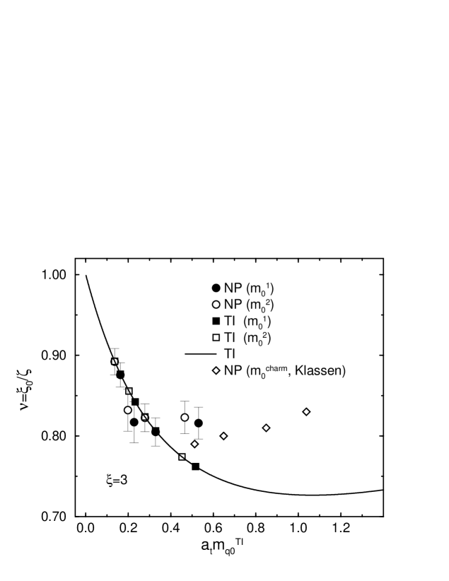
FIG. 9.: The tadpole improved bare mass $\tilde{m_{0}}\equiv a_{t}m_{q0}^{\rm TI}$ versus $\nu=\xi_{0}/\zeta$ at $\xi=3$. ‘TI’ and ‘NP’ denote the tree level tadpole improved value and nonperturbative value respectively. Circles and squares are our data at $m_{0}=m_{0}^{1},m_{0}^{2}\ (\approx m_{0}^{\rm charm})$ for $\beta=5.7$-6.35. The error bars for the circles denote the statistical uncertainty of $\nu^{\rm NP}=\xi_{0}/\zeta^{\rm NP}$. We also plot Klassen’s data at $m_{0}=m_{0}^{\rm charm}$ for $\beta=5.5$-5.8 as open diamonds.

FIG. 10.: Results of $r_{0}/a_{s}$. The left figure shows typical fit range ($r_{\rm min}$) dependence of $r_{0}/a_{s}$ and its averaged value. The right is the result of $a_{s}/r_{0}$ as a function of $\beta$ and its fit curve Eq. (62).

FIG. 11.: The left-hand side shows $\beta$-dependence of the lattice spacing. The solid line is the fit curve Eq. (62), while dotted and dashed lines are spline interpolations to square and triangle symbols respectively. On the right-hand side $a_{s}^{1\bar{P}-1\bar{S}}/a_{s}^{r_{0}}$ and $a_{s}^{2\bar{S}-1\bar{S}}/a_{s}^{r_{0}}$ as a function of $a_{s}^{r_{0}}$ are plotted.

FIG. 12.: Comparison of results for various $(M_{\rm lat},\zeta)$ tunings. The scale is set by $r_{0}$. The data points are slightly shifted along the horizontal axis for the distinguishability.

FIG. 13.: Charmonium spectrum at finite $\beta$. The scale is fixed from $r_{0}$, $\Delta M(1\bar{P}-1\bar{S})$ and $\Delta M(2\bar{S}-1\bar{S})$.

FIG. 14.: S-state hyperfine splitting $\Delta M(1^{3}S_{1}-1^{1}S_{0})$. Results obtained with $\tilde{c_{s}}=u_{s}^{3}c_{s}=1$ are collected here. Our results are shown by filled symbols for each input, while results by Klassen (set B) and Chen (set C) with the $r_{0}$ input are shown by open symbols. In the legend, we give the choice of the anisotropy $\xi$, $\zeta$ tuning, tadpole factor and scale input. These captions also apply to the figures that follow.

FIG. 15.: P-state fine structure splitting $\Delta M(1^{3}P_{1}-1^{3}P_{0})$.

FIG. 16.: P-state fine structure splitting $\Delta M(1^{3}P_{2}-1^{3}P_{1})$.

FIG. 17.: Fine structure ratio $\Delta M(1^{3}P_{2}-1^{3}P_{1})/\Delta M(1^{3}P_{1}-1^{3}P_{0})$.

FIG. 18.: Splitting $\Delta M(1^{1}P_{1}-1^{3}P)$.

FIG. 19.: Spin averaged $1\bar{P}-1\bar{S}$ splitting. In the figures, we always omit the bar for the spin average.

FIG. 20.: Spin dependent $1P-1\bar{S}$ splittings.

FIG. 21.: Spin averaged $2\bar{S}-1\bar{S}$ splitting.

FIG. 22.: Spin dependent $2S-1S$ splittings.

FIG. 23.: Spin dependent $2P-1P$ splittings.

FIG. 24.: Charmonium spectrum in the continuum limit. The scale is set by $1\bar{P}-1\bar{S}$ splitting.

FIG. 25.: $R_{\rm HFS}$ with $\tilde{c_{s}}=1/\nu$ and $\zeta=\zeta^{\rm NP}$ at $\xi=3$ and 2. The thick symbols are the results with $m_{q}=\tilde{m_{1}}$, while the thin symbols are those with $m_{q}=\tilde{m_{2}}$. The results with $\tilde{c_{s}}=1/\nu$ but $\zeta=\zeta^{\rm TI}$ (where $m_{q}=\tilde{m_{1}}=\tilde{m_{2}}$) are also shown by the dotted line ($\xi=3$) and dashed line ($\xi=2$).

FIG. 26.: Klassen’s results of S-state hyperfine splitting $\Delta M(1^{3}S_{1}-1^{1}S_{0})$ with $\tilde{c_{s}}=1/\nu$ and $\zeta=\zeta^{\rm NP}$ (set D). The scale is set by $r_{0}$. Lines denote $a_{s}^{2}$-linear extrapolations.

FIG. 27.: $R_{\rm HFS}$ with $\tilde{c_{s}}=1$. Here $m_{q}=\tilde{m_{1}}$. The stars are slightly shifted along the horizontal axis for the distinguishability.

FIG. 28.: The results of S-state hyperfine splitting $\Delta M(1^{3}S_{1}-1^{1}S_{0})$ with $\tilde{c_{s}}=1$. The scale is set by $r_{0}$.

REFERENCES

- [1] B. A. Thacker and G. P. Lepage, Phys. Rev. D 43, 196 (1991).
- [2] G. P. Lepage, L. Magnea, C. Nakhleh, U. Magnea and K. Hornbostel, Phys. Rev. D 46, 4052 (1992) [arXiv:hep-lat/9205007].
- [3] C. T. Davies, K. Hornbostel, A. Langnau, G. P. Lepage, A. Lidsey, J. Shigemitsu and J. H. Sloan, Phys. Rev. D 50, 6963 (1994) [arXiv:hep-lat/9406017].
- [4] C. T. Davies, K. Hornbostel, G. P. Lepage, A. Lidsey, P. McCallum, J. Shigemitsu and J. H. Sloan [UKQCD Collaboration], Phys. Rev. D 58, 054505 (1998) [arXiv:hep-lat/9802024].
- [5] H. D. Trottier, Phys. Rev. D 55, 6844 (1997) [arXiv:hep-lat/9611026].
- [6] N. H. Shakespeare and H. D. Trottier, Phys. Rev. D 58, 034502 (1998) [arXiv:hep-lat/9802038].
- [7] T. Manke, I. T. Drummond, R. R. Horgan and H. P. Shanahan [UKQCD Collaboration], Phys. Rev. D 57, 3829 (1998) [arXiv:hep-lat/9710083].
- [8] T. Manke et al. [CP-PACS Collaboration], Phys. Rev. Lett. 82, 4396 (1999) [arXiv:hep-lat/9812017].
- [9] T. Manke et al. [CP-PACS Collaboration], Phys. Rev. D 62, 114508 (2000) [arXiv:hep-lat/0005022].
- [10] T. Manke et al. [CP-PACS Collaboration], Phys. Rev. D 64, 097505 (2001) [arXiv:hep-lat/0103015].
- [11] A. X. El-Khadra, A. S. Kronfeld and P. B. Mackenzie, Phys. Rev. D 55, 3933 (1997) [arXiv:hep-lat/9604004].
- [12] B. Sheikholeslami and R. Wohlert, Nucl. Phys. B 259, 572 (1985).
- [13] Z. Sroczynski, Nucl. Phys. Proc. Suppl. 83-84, 971 (2000) [arXiv:hep-lat/9910004].
- [14] S. Aoki et al. [JLQCD Collaboration], Phys. Rev. Lett. 80 (1998) 5711.
- [15] A. X. El-Khadra, A. S. Kronfeld, P. B. Mackenzie, S. M. Ryan and J. N. Simone, Phys. Rev. D 58, 014506 (1998) [arXiv:hep-ph/9711426].
- [16] C. W. Bernard et al., Phys. Rev. Lett. 81, 4812 (1998) [arXiv:hep-ph/9806412].
- [17] A. Ali Khan et al. [CP-PACS Collaboration], Phys. Rev. D 64, 034505 (2001) [arXiv:hep-lat/0010009].
- [18] T. R. Klassen, Nucl. Phys. Proc. Suppl. 73, 918 (1999) [arXiv:hep-lat/9809174].
- [19] T.R. Klassen, unpublished.
- [20] C. J. Morningstar and M. J. Peardon, Phys. Rev. D 56, 4043 (1997) [arXiv:hep-lat/9704011].
- [21] C. J. Morningstar and M. J. Peardon, Phys. Rev. D 60, 034509 (1999) [arXiv:hep-lat/9901004].
- [22] J. Harada, A. S. Kronfeld, H. Matsufuru, N. Nakajima and T. Onogi, Phys. Rev. D 64, 074501 (2001) [arXiv:hep-lat/0103026].
- [23] S. Aoki, Y. Kuramashi and S. Tominaga, arXiv:hep-lat/0107009.
- [24] P. Chen, Phys. Rev. D 64, 034509 (2001) [arXiv:hep-lat/0006019].
- [25] The experimental values are taken from C. Caso et al. [Particle Data Group Collaboration], Eur. Phys. J. C 3, 1 (1998).
- [26] A. Ali Khan et al. [CP-PACS Collaboration], Nucl. Phys. Proc. Suppl. 94, 325 (2001) [arXiv:hep-lat/0011005].
- [27] S. Aoki et al. [CP-PACS Collaboration], arXiv:hep-lat/0110129.
- [28] M. Fujisaki et al. [QCD-TARO Collaboration], Nucl. Phys. Proc. Suppl. 53, 426 (1997) [arXiv:hep-lat/9609021].
- [29] T. R. Klassen, Nucl. Phys. B 533, 557 (1998) [arXiv:hep-lat/9803010].
- [30] J. Engels, F. Karsch and T. Scheideler, Nucl. Phys. B 564, 303 (2000) [arXiv:hep-lat/9905002].
- [31] G. P. Lepage and P. B. Mackenzie, Phys. Rev. D 48, 2250 (1993) [arXiv:hep-lat/9209022].
- [32] R. Sommer, Nucl. Phys. B 411, 839 (1994) [arXiv:hep-lat/9310022].
- [33] G. S. Bali and K. Schilling, Phys. Rev. D 46, 2636 (1992).
- [34] G. S. Bali and K. Schilling, Phys. Rev. D 47, 661 (1993) [arXiv:hep-lat/9208028].
- [35] S. Aoki et al. [CP-PACS Collaboration], Phys. Rev. D 60, 114508 (1999) [arXiv:hep-lat/9902018].
- [36] C. R. Allton, arXiv:hep-lat/9610016.
- [37] For example, see, W. Lucha, F. F. Schoberl and D. Gromes, Phys. Rept. 200, 127 (1991).