Glueballs, strings and topology in SU(N) gauge theory

Abstract

I show how one can use lattice methods to calculate various continuum properties of SU($N$) gauge theories; in part to explore old ideas that $N=3$ might be close to $N=\infty$. I describe calculations of the low-lying ‘glueball’ mass spectrum, of the string tensions of $k$-strings and of topological fluctuations for $2\leq N\leq 5$. We find that mass ratios appear to show a rapid approach to the large–$N$ limit, and, indeed, can be described all the way down to SU(2) using just a leading $O(1/N^{2})$ correction. We confirm that the smooth large–$N$ limit we find is confining and is obtained by keeping a constant ’t Hooft coupling. We find that the ratio of the $k=2$ string tension to the $k=1$ fundamental string tension is much less than the naive (unbound) value of 2 and is considerably greater than the naive bag model prediction; in fact it is consistent, within quite small errors, with either the M(-theory)QCD-inspired conjecture that $\sigma_{k}\propto\sin(\pi k/N)$ or with ‘Casimir scaling’. Finally I describe calculations of the topological charge of the gauge fields. We observe that, as expected, the density of small-size instantons vanishes rapidly as $N$ increases, while the topological susceptibility appears to have a non-zero $N=\infty$ limit.

1 INTRODUCTION

How SU($N$) gauge theories approach their $N=\infty$ limit and what that limit is, are interesting questions [1], in themselves, whose answers would, in addition, represent a significant step towards addressing the same question in the context of QCD. Accurate lattice calculations in 2+1 dimensions [2] show that in that case the approach is remarkably precocious in that even $N=2$ is close to $N=\infty$. Such calculations have to be very accurate because for each value of $N$ one has to perform a continuum extrapolation of various mass ratios and then these are compared and extrapolated to $N=\infty$. Earlier D=3+1 calculations [3, 4] were much too rough for this purpose even if their message was optimistic. Recently, however, this situation has been rapidly improving and here I want to describe some of the things that one has already learned.

Analyses of Feynman diagrams to all orders imply [1], that the SU($N$) theory will have a smooth limit if we keep fixed the ’t Hooft coupling

$$\lambda\equiv g^{2}N.$$ (1)

We would like a non-perturbative confirmation of this expectation. Again, we would like a confirmation of the assumption that the large-$N$ theory remains confining, since much of the phenomenological argument that QCD might be close to $N=\infty$ relies on this being so [1]. Since quarks are in the fundamental representation, the leading correction to $N=\infty$ is expected to be $O(1/N)$. In the pure gauge theory it is expected to be $O(1/N^{2})$. (Again an expectation that one would wish to test non-perturbatively.) Thus if QCD is close to $N=\infty$ one would expect the SU(3) gauge theory to be close to SU($\infty$) as well. We can test this by calculating dimensionless ratios of physical masses as a function of $N$. There are also arguments and speculations (e.g. [5]) that topological fluctuations are very different at large $N$ and at small $N$; this too we would like to test in lattice simulations.

The calculations [6, 7] on glueballs, topology and $k$-strings which I will describe have been performed in collaboration with Biagio Lucini. The strategy is simple: we calculate the relevant (continuum) properties of SU(2), SU(3), SU(4) and SU(5) theories and directly compare them. Since $N=5$ is large in the sense that the leading correction $\propto 1/N^{2}=1/25\ll 1$, it is not surprising that such a calculation turns out to suffice for our purposes. These calculations were intended as exploratory. A much larger calculation is now underway and this will provide much more information on the mass spectrum and its dependence on the number of colours.

2 FROM LATTICE TO PHYSICS

Our lattice calculations are entirely standard [6, 7]. The Euclidean space-time lattice is hypercubic with periodic boundary conditions.The degrees of freedom are SU($N$) matrices residing on the links of the lattice. In the partition function the fields are weighted with $\exp\{S\}$ where $S$ is the standard plaquette action

$$S=-\beta\sum_{p}\biggl{(}1-{1\over N}ReTr\,U_{p}\biggr{)},$$ (2)

in which $U_{p}$ is the ordered product of the matrices on the boundary of the plaquette $p$. For smooth fields this action reduces to the usual continuum action with $\beta=2N/g^{2}$. For rough fields on a lattice of spacing $a$ we can define a running lattice coupling $g_{L}(a)$ which reduces in the continuum limit to a coupling $g(a)$ in our favourite scheme:

$$\beta\equiv{{2N}\over{g_{L}^{2}(a)}}\stackrel{{\scriptstyle a\to 0}}{{\longrightarrow}}{{2N}\over{g^{2}(a)}}$$ (3)

Thus by varying the inverse lattice coupling $\beta$ we can vary the lattice spacing $a$.

To calculate a mass we construct some operator $\phi(t)$ with the quantum numbers of the state (typically this will be a linear combination of the products of link matrices around some closed loops) and then use the standard decomposition of the Euclidean correlator in terms of energy eigenstates

$$C(t)=\langle\phi^{\dagger}(t)\phi(0)\rangle=\sum_{n}|\langle\Omega|\phi|n\rangle|^{2}\exp\{-E_{n}t\}$$ (4)

where $|n\rangle$ are the energy eigenstates, with $E_{n}$ the corresponding energies, and $|\Omega\rangle$ is the vacuum state. We evaluate the corresponding Feynman Path Integrals using standard Monte Carlo techniques. On the lattice $t=na$ and so we obtain the energies from eqn(4) as $aE_{n}$ i.e. in units of the lattice spacing. In practice one needs to use several carefully chosen operators, and a variational calculation [6, 7]. Since our volume is finite we must make sure that finite volume corrections are negligible. For the calculations I describe here such checks have been made.

Having calculated some masses $am_{i}$ at a fixed value of $a$ (i.e. at a fixed value of $\beta$) we can remove lattice units by taking ratios: $am_{i}/am_{j}=m_{i}/m_{j}$. This ratio differs from the desired continuum value by lattice corrections. For our action the functional form of the leading correction is known to be $O(a^{2})$. Thus for small enough $a$ we can extrapolate our calculated mass values

$${{m_{i}(a)}\over{m_{j}(a)}}={{m_{i}(0)}\over{m_{j}(0)}}+ca^{2}m^{2}_{k}(a)$$ (5)

where using different $m_{k}$ will make differences at $O(a^{4})$ (as does the $a$-dependence of $m_{k}(a)$). We shall later show some explicit examples of such extrapolations.

Having calculated such mass ratios in various continuum SU($N$) gauge theories, we can attempt to extrapolate to $N=\infty$ using the fact that the leading correction is expected to be $O(1/N^{2})$:

$$\left.{{m_{i}}\over{m_{j}}}\right|_{N}=\left.{{m_{i}}\over{m_{j}}}\right|_{\infty}+{c_{ij}\over N^{2}}.$$ (6)

If such fits are good for $N\geq N_{0}$ then we may regard SU($N_{0}$) as being close to SU($\infty$).

3 GLUEBALLS

In this exploratory calculation we focus on what are expected (from previous calculations in SU(2) and SU(3) [9, 10]) to be the lightest states: the lightest $J^{PC}=0^{++}$ and $2^{++}$ glueballs. We also calculate the mass of the first excited scalar glueball, which we shall refer to as the $0^{++\star}$. In addition to these glueball masses we calculate the string tension, $a^{2}\sigma$, of the flux tube between static sources in the fundamental representation (see the next Section.). This last is our most accurately calculated quantity and so we use it to form the dimensionless mass ratios $m/\surd\sigma$ which we extrapolate to the continuum limit using eqn(5). In Fig.1 I show you how this works for the lightest scalar glueball for $N=2,3,4,5$.

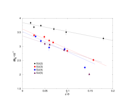
Figure 1: The mass of the lightest scalar glueball, $m_{0^{++}}$, expressed in units of the string tension, $\sigma$, is plotted against the latter in lattice units. The $a\to 0$ continuum extrapolation, using a leading lattice correction, is shown.

While the mass of the scalar glueball is the most accurately calculated, because it is the lightest, it is also the one with (by far) the largest lattice corrections. Despite this it is already clear from Fig.1 that for small $a$ there is very little $N$-dependence for $N\geq 3$. To be quantitative we perform continuum extrapolations using eqn(5), as shown in Fig.1. The results are shown in Fig.2

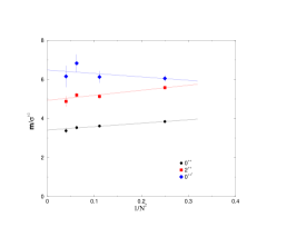
Figure 2: Continuum scalar, tensor and excited scalar masses expressed in units of the string tension and plotted against $1/N^{2}$. Linear extrapolations to $N=\infty$ are shown in each case.

where we also show the extrapolations to $N=\infty$ using eqn(6).

We see from Fig.2 that, as far as the lightest glueballs are concerned, all SU($N$) theories can be described by a modest leading $O(1/N^{2})$ correction to the SU($\infty$) limit.

We also see from these plots that the ratio of the glueball masses to the (square root of) the string tension has a finite non-zero limit as $N\to\infty$. This tells us that the confining string tension remains finite and non-zero as $N\to\infty$. (Caution: numerical calculations only test confinement to some finite distance – which in the case of our higher-$N$ calculations is not yet very large.)

4 ’T HOOFT COUPLING

The analysis of diagrams [1] suggests that the way to achieve a smooth limit as $N\to\infty$ is by keeping the ’t Hooft coupling, $\lambda\equiv g^{2}N$, constant. Since the coupling runs, we should say that what we keep fixed is the running ’t Hooft coupling, as defined on some scale $l$ that is fixed in units of some quantity that partakes of the smooth large-$N$ limit, such as the string tension. To do this we use eqn(3) which tells is that a suitable defintion of a running ’t Hooft coupling is

$$\lambda_{I}(a)=g_{I}^{2}(a)N={{2N^{2}}\over{\beta\langle ReTr\,U_{p}/N\rangle}}$$ (7)

The extra factor involving the plaquette is a mean-field (or tadpole) improved version of $\beta$ and the naive $\lambda(a)$ we would derive from it [11]. It is necessary [11] because the naive lattice coupling is known to be very poor in the sense of having very large higher order corrections.

We extract $\lambda_{I}(a)$ for each of our various lattice calculations at various $N$ and $a$ . Our diagrammatic expectation is that if we plot $a\surd\sigma$ against $\lambda_{I}(a)$ then, for large enough $N$, the calculated values should fall on a universal curve. In Fig.3 we plot all our calculated values of $a\surd\sigma$, against the value of $\lambda_{I}(a)$. We observe that, within corrections which are small except at the largest value of $a$, we do indeed see a universal curve, and so the diagrammatic expectation is supported by our non-perturbative calculations [6].

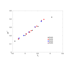
Figure 3: The square root of the string tension in lattice units, $a\surd\sigma$, plotted against the ’t Hooft coupling, $\lambda_{I}\equiv g^{2}_{I}N$.

5 STRINGS

In a confining SU($N$) gauge theory, the potential between two static charges in the fundamental representation is expected to grow linearly at large separations as $V(r)=\sigma r$ where $\sigma$ is the fundamental string tension. If we have charges in other representations then, in SU(3), they can be screened to either the fundamental or the trivial representation by gluons from the vacuum. So the fundamental string is the only stable one (assuming it to have the lowest tension). In SU($N\geq 4$) there are other stable strings. It is convenient to label a charge by the integer $k$ if its wave function transforms by a factor of $z^{k}$ under a global gauge transformation $z$ belonging to the centre $Z_{N}$ of the group. Because gluons transform trivially under the centre, they cannot screen a charge of $k$ into a charge of $k^{\prime}$ if $z^{k}\neq z^{k^{\prime}}$. Thus there should be a different stable string for each such $k$, with string tension $\sigma_{k}$. (Conjugate strings will have the same tensions.) Of course, it might be that we just have $k$ fundamental strings joining such sources, in which case one will find $\sigma_{k}=k\sigma$ and we have no new string. As we shall see, this is not the case: we find new tightly bound $k$-strings. The first $k=2$ string appears in SU(4) and the first $k=3$ one in SU(6). The values of $\sigma_{k}$ are interesting because they carry information about confinement. Also because there are specific conjectures about their values from M(-theory)QCD [8], from arguments about Casimir scaling [12], and from certain models, such as the bag model [13]. Moreover such strings may have striking implications [6, 7] for the glueball mass spectrum as a function of $N$.

The simplest way to calculate $\sigma_{k}$ is by calculating the mass of a $k$-string that winds around a spatial torus. In a confining theory it cannot break and will have a length $l=aL$ (on an $L^{3}$ spatial lattice). For long enough strings, the mass of such a loop is given by

$$m_{k}(l)\stackrel{{\scriptstyle l\to\infty}}{{\simeq}}\sigma_{k}l-{{\pi(D-2)}\over{6}}{c_{s}\over l}.$$ (8)

where the $O(1/l)$ correction is the Casimir energy of a periodic string and $c_{s}$ is proportional to the central charge. This correction is universal [14] since it depends only upon the massless modes in the effective string theory and does not depend upon the detailed and complicated dynamics of the flux tube on scales comparable to its width. The central charge is given [15] by the number of massless bosonic and fermionic modes that propagate along the string. In practice it is usually assumed that $c_{s}=1$, corresponding to the simplest possible (Nambu-Goto) bosonic string theory. However, these modes are not related to the fundamental degrees of freedom of our SU($N$) gauge theory in any transparent way and the presence of fermionic modes is certainly not excluded. Direct numerical evidence is hard to get since we are interested in small corrections to long, massive strings. In Fig.4 we show the effective value of $c_{s}$ that one obtains [7] by fitting the masses of two strings of different lengths (as indicated) to eqn(8) in SU(2) and for a lattice spacing $a\simeq 0.16/\surd\sigma\simeq 0.07fm$. This provides some evidence for the simple bosonic string correction for lengths $l\geq 1.2fm$.

Figure 4: The D=3+1 effective string correction coefficient estimated from the masses of flux loops of different lengths (indicated by the span of the horizontal error bar). The solid line is what one expects for a simple bosonic string. For comparison the dashed line indicates the value for the Neveu-Schwartz string.

Assuming, then, eqn(8) with $c_{s}=1$ we obtain from our calculated loop masses the string tensions shown in Fig.5,

Figure 5: The ratio of $k=2$ and $k=1$ string tensions in our D=3+1 SU(4) ($\bullet$) and SU(5) ($\circ$) lattice calculations plotted as a function of $a^{2}\sigma$. Extrapolations to the continuum limit, using a leading $O(a^{2})$ correction, are displayed.

from which we obtain

$$\lim_{a\to 0}{{\sigma_{\mathit{k=2}}}\over{\sigma}}=\left\{\begin{array}[]{ll}1.357\pm 0.029&\ \ \ {\mathrm{SU(4)}}\\ 1.583\pm 0.074&\ \ \ {\mathrm{SU(5)}}\end{array}\right..$$ (9)

Clearly the $k=2$ string is tightly bound, and the string tension is incompatible, for example, with the naive bag model. What we find is that it falls between the MQCD and Casimir scaling predictions and, at the two sigma level, is consistent with both. We remark that a very recent higher statistics calculation [16] favours MQCD over Casimir scaling.

6 TOPOLOGY

Gauge fields in four (suitably compactified) Euclidean dimensions possess non-trivial topological properties characterised by an integer topological charge $Q$. Topological fluctuations break the (approximate) $U_{A}(1)$ symmetry of QCD, thus leading [17] to the non-Goldstone character of the $\eta^{\prime}$. One can argue that if $N=3$ is close to $N=\infty$ one can relate [18] the mass of the $\eta^{\prime}$ to the topological susceptibility

$$\chi_{t}\equiv{{\langle Q^{2}}\rangle\over V},$$ (10)

of the gauge theory without quarks. ($V$ is the space-time volume.) This suggests a value $\chi_{t}\simeq(180MeV)^{4}$, which is indeed close to what one finds in pure gauge theories [19]. All this fits together if we can show that the $N=3$ values of the pure gauge susceptibility and of $Nm^{2}_{\eta^{\prime}}$ are close to their $N=\infty$ values. While we cannot say much about the latter, we can and shall address the former.

We calculate $Q$ for our lattice fields by standard cooling methods which for this purpose are reliable [19]. These calculations are performed simultaneously with the glueball calculations discussed earlier and the values of $\chi^{1/4}_{t}/\surd\sigma$ are extrapolated to the continuum limit with an $a^{2}\sigma$ correction, following eqn(5). The resulting continuum values are plotted against $1/N^{2}$ in Fig.6

Figure 6: The continuum topological susceptibility in units of the string tension plotted against $1/N^{2}$. A linear extrapolation to $N=\infty$ is shown.

We observe that, just as for the glueball masses, the $N$-dependence is well described by a modest $O(1/N^{2})$ correction and the topological susceptibility, expressed in physical units, does not differ greatly when we go from $N=3$ to $N=\infty$.

These conclusions are somewhat weaker here than for the glueballa because of the rapidly growing errors as $N$ increases. The reason for this turns out to be interesting and easy to see [6]. As $N$ grows isolated instantons become increasingly unlikely. This is because of the factor in the instanton density

$$D(\rho)d\rho\propto{{d\rho}\over{\rho}}{1\over{\rho^{4}}}\Biggl{\{}{{b^{2}}\over{\lambda^{2}(\rho)}}e^{-{{8\pi^{2}}\over{\lambda(\rho)}}}\Biggr{\}}^{N}.$$ (11)

where $\lambda$ is the ’t Hooft coupling that we keep fixed as $N\to\infty$. In the real vacuum this argument holds for instantons with $\rho\ll 1$ ‘fermi’ and so these instantons are exponentially suppressed as $N$ increases. Now the Monte Carlo changes $Q$ by an instanton shrinking through small values of $\rho$ down to $\rho\sim a$ where it can vanish through the lattice. (Or the reverse process.) However eqn(11) tells us that the probability of a very small instanton goes rapidly to zero as $N$ grows. Thus the lattice fields rapidly become constrained to lie in given topological sectors and for this quantity the Monte Carlo rapidly ceases to be ergodic as $N$ grows, and the stattistical errors on $\langle Q^{2}\rangle$ grow rapidly – as observed.

We can attempt to calculate $D(\rho)$ and so see this effect directly. To do so we examine the topological charge density on the cooled fields and associate an instanton to each peak in this density using the semiclassical formula

$$Q_{peak}={6\over{\pi^{2}\rho^{4}}}.$$ (12)

This procedure is clearly of ambiguous validity for broad instantons, but is unambiguous for the high narrow peaks that correspond to the smaller instantons of interest to us here. In Fig.7 we display the result of such a calculation, comparing the instanton densities in SU(2), SU(3) and SU(4) on lattices with (almost) equal volumes and lattice spacings when expressed in units of the string tension. We clearly see a drastic suppression of small instantons with increasing $N$.

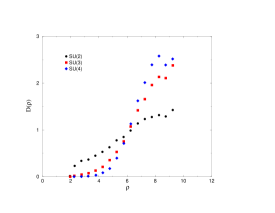
Figure 7: The number density of topological charges plotted as a function of the charge radius, $\rho$; obtained for $N=2,3,4$ from $20^{4}$ lattices with $a\surd\sigma\sim 0.16$.

7 CONCLUSIONS

We saw above that, as far as the lightest glueballs, string tensions and topological susceptibility are concerned, all SU($N$) theories can be described by a modest leading $O(1/N^{2})$ correction to the SU($\infty$) limit. In this sense we can say that not only is $N=3$ close to $N=\infty$ but so is $N=2$.

The large amount of interesting physics delivered by these modest (workstation) calculations, provides a strong motivation for going further. Currently we [20] are starting much larger calculations on anisotropic lattices, which will enable us to obtain accurate mass estimates for a much larger range of glueball states and very accurate string tension ratios. Simultaneously we [21] are using overlap fermions [22] to determine the relationship between topology and chiral symmetry breaking as a function of $N$; and to say something about instantons and topology at large $N$. A more ambitious project, which would require the use of one of the larger $\sim 1$ teraflop resources that are becoming available to many groups, would be to calculate the quenched hadron spectrum at large $N$ – which is interesting since it approaches the correct spectrum of SU($N$) QCD as we take $N\to\infty$ at fixed non-zero quark mass. And then, eventually, to dynamical quarks at large $N$ and the $\eta^{\prime}$ …

References

-
[1]
G. ’t Hooft, Nucl. Phys. B72 (1974) 461.
E. Witten, Nucl. Phys. B160 (1979) 57.
S. Coleman, 1979 Erice Lectures.
A. Manohar, 1997 Les Houches Lectures, hep-ph/9802419. - [2] M. Teper, Phys. Rev. D59 (1999) 014512.
- [3] M. Teper, Phys. Lett. B397 (1997) 223. and unpublished.
- [4] M. Wingate and S. Ohta, hep-lat/0006016; Nucl. Phys. Proc. Suppl. 83 (2000) 381.
- [5] E. Witten, Nucl. Phys. B149 (1979) 285.
- [6] B. Lucini and M. Teper, JHEP 0106 (2001) 050.
- [7] B. Lucini and M. Teper, Phys. Lett. B501 (2001) 128; Phys.Rev. D64 (2001) 105019.
-
[8]
A. Hanany, M. J. Strassler and A. Zaffaroni,
Nucl. Phys. B513 (1998) 87.
M. J. Strassler, Nucl. Phys. Proc. Suppl. 73 (1999) 120. - [9] M. Teper, hep-th/9812187.
- [10] C. Morningstar and M. Peardon, Phys. Rev. D56 (1997) 4043; Phys. Rev. D60 (1999) 034509.
-
[11]
G. Parisi,
in High Energy Physics - 1980 (AIP 1981).
P. Lepage and P. Mackenzie, Phys. Rev. D48 (1993) 2250.
P. Lepage, Schladming Lectures, hep-lat/9607076. -
[12]
J. Ambjorn, P. Olesen and C. Peterson,
Nucl. Phys. B240 (1984) 189, 533; B244 (1984) 262;
Phys. Lett. B142 (1984) 410.
S. Deldar, Phys. Rev. D62 (2000) 034509; JHEP 0101 (2001) 013.
G. Bali, Phys. Rev. D62 (2000) 114503.
V. Shevchenko and Yu. Simonov, Phys. Rev. Lett. 85 (2000) 1811; hep-ph/0104135. -
[13]
K. Johnson and C. B. Thorn,
Phys. Rev. D13 (1976) 1934.
T. H. Hansson, Phys. Lett. B166 (1986) 343. - [14] M. Lüscher, K. Symanzik and P. Weisz, Nucl. Phys. B173 (1980) 365.
- [15] J. Polchinski, String Theory, Vol I and II (CUP, 1998).
- [16] L. Del Debbio, H. Panagopoulos, P. Rossi and E. Vicari, hep-th/0106185; hep-th/0111090.
- [17] G. ’t Hooft, Physics Reports 142 (1986) 357.
-
[18]
E. Witten,
Nucl. Phys. B156 (1979) 269.
G. Veneziano, Nucl. Phys. B159 (1979) 213. - [19] M. Teper, Nucl. Phys. Proc. Suppl. 83 (2000) 146.
- [20] B. Lucini, M. Teper and U. Wenger, in progress.
- [21] N. Cundy, M. Teper and U. Wenger, in progress.
- [22] H. Neuberger, these proceedings.