A nonperturbative determination of the $O(a)$ improvement coefficient $c_{A}$ and the scaling of $f_{\pi}$ and $m^{\overline{MS}}$.

Abstract

We report on an investigation of the LANL method for determining the $O(a)$ improvement coefficient $c_{A}$ nonperturbatively. We find we are able to extract reliable estimates for the coefficient using this method. However, our study of systematic errors shows that for very accurate determinations of $c_{A}$, the smearing function must be tuned and the volume fixed to keep the $O(a)$ ambiguity in $c_{A}$ fixed as $\beta$ varies. Consistency was found with previous results from the LANL group and (within fairly large errors) 1-loop perturbation theory; $c_{A}$ does not change significantly over the range $\beta=5.93{-}6.2$. The big difference between our results and those of the ALPHA collaboration, around $\beta=6.0$, show that the $O(a)$ differences in $c_{A}$ between the different methods can be large. We find that the lattice spacing dependence of $f_{\pi}$ and the renormalised quark mass is much smaller using our values of the coefficient compared to those of the ALPHA collaboration.

I Introduction

The use of Symanzik improvement [1] of lattice actions and matrix elements is widespread and very effective. However, with each improvement term added the corresponding coefficient must be determined to enable discretisation effects to be reduced to the desired level. Considering the light hadron spectrum and matrix elements, the relevant $O(a)$ improvement coefficients are, for the most part, only known to $1$-loop in perturbation theory, leaving residual $O(\alpha^{2}a)$ discretisation terms. A nonperturbative determination of these coefficients is desirable to completely remove $O(a)$ effects. Such a determination is possible through the imposition of the axial Ward identities (AWI) on the lattice.

Central to a programme of determining $O(a)$ improvement coefficients nonperturbatively is the calculation of $c_{A}$, the improvement coefficient of the axial-vector current; the improved current appears in the expression for the generic axial Ward identity and $c_{A}$ must be determined before other operator improvement coefficients can be calculated [2]. So far, two groups, the LANL group [3, 2, 4] and the ALPHA collaboration [5, 6], have calculated $c_{A}$ along with several other improvement coefficients.

Their results for $c_{A}$ at $\beta=6.0$ and $6.2$ are summarised in figure 1 and compared with 1-loop perturbation theory (using $\alpha=\alpha_{P}(1/a)$ [7]). While the results are compatible on the finer lattice, there is a big difference in the values for $\beta=6.0$. This difference can be explained by the $O(a)$ ambiguity which exists in nonperturbative determinations of $O(a)$ improvement coefficients. As long as the improvement conditions for each determination are applied consistently as $\beta$ changes, differences in the value of $c_{A}$ are not important in principle; the difference will disappear in the continuum limit.

In practice, different values of $c_{A}$ can have a large effect away from the continuum limit. This is because the matrix elements appearing at $O(a)$ for $f_{\pi}$ and the renormalised quark mass are numerically large compared to the leading order term.

$$f^{imp} = \left<P|A_{4}|0\right>+c_{A}\left<P|a\partial_{4}P|0\right>$$ (1)

$$m_{PCAC}^{imp} = \frac{\left<P|\partial_{4}A_{4}|0\right>}{2\left<P|P|0\right>}+c_{A}\frac{\left<P|a\partial_{4}^{2}P|0\right>}{2\left<P|P|0\right>},$$ (2)

and $a\left<P|\partial_{4}P|0\right>/\left<P|A_{4}|0\right>\sim aM_{\pi}^{2}/m_{q}$. An $O(a)$ ambiguity in $c_{A}$ therefore appears at $O(a^{2})$ but multiplied by a large matrix element and it is undesirable to have large $O(a^{2})$ scaling violations, even if $O(a)$ errors have been removed.

Our aim is to investigate how well $c_{A}$ is determined using the LANL method. The latter only requires a conventional analysis, which is available from simulations performed for spectroscopic calculations, compared to using the Schrödinger functional techniques of the ALPHA collaboration. With significantly higher statistics than those of reference [2] we are able to improve on the LANL analysis by performing correlated fits, investigating the choice of lattice derivatives employed more widely and determining the stability of the LANL results to changes in the fitting range. In addition, we study the scaling behaviour of $f_{\pi}$ and the renormalised quark mass with respect to the choice made for $c_{A}$.

The paper is organised as follows: in section II we outline how to extract $c_{A}$ from the PCAC relation and in particular the method employed by the LANL group. Results are presented in section III, which includes a comparison of our results with those of the LANL group and the ALPHA collaboration. The scaling of $f_{\pi}$ and the renormalised quark mass is dealt with in section IV, followed by the conclusions in section V. Technical details not directly related to the method of calculating $c_{A}$ - the simulation details, extracting meson masses and decay constants, the renormalisation factors used to obtain $f_{\pi}$ and $m^{\overline{MS}}$ and the chiral extrapolations are all given in the Appendix.

II $c_{A}$ from the PCAC relation

The PCAC relation in euclidean space can be written as

$$\left<J\partial_{\mu}A_{\mu}(x)\right>=2m_{PCAC}\left<JP(x)\right>$$ (3)

and should hold on the lattice for all $x$ not coincident with $J$ up to discretisation terms. The axial-vector current, $A_{\mu}$, is given by $\bar{\psi}\gamma_{\mu}\gamma_{5}\psi$, the pseudoscalar operator $P=\bar{\psi}\gamma_{5}\psi$ and $J$ is any operator with the pseudoscalar quantum numbers. $m_{PCAC}$ is the bare current quark mass. For simplicity we sum over position space, restricting ourselves to zero momentum, and define

$$r_{J}(t) = \frac{<J\partial_{4}A_{4}(t)>}{<JP(t)>}.$$ (4)

Thus, equation 3 becomes

$$r_{J}(t)=m(t)=2m_{PCAC}+O(a).$$ (5)

This relation holds for all states (ground and radial excitations) of the pseudoscalar meson. In the limit of large times, when only the ground state contributes to $r_{J}$, then $m(t)$ is a constant given by $2m_{PCAC}+O_{g.s.}(a)$, where $O_{g.s.}(a)$ are the discretisation errors associated with the ground state. At earlier times, when excited states make a significant contribution (with different discretisation errors), $m(t)$ becomes time dependent, as can be seen in figure 2.

The size of the discretisation terms (and the time dependence of $m(t)$) are reduced to $O(a^{2})$ when we improve the axial-vector current 

$$A_{4}\rightarrow A_{4}^{I}=A_{4}+ac_{A}\partial_{4}P+O(a^{2}).$$ (6)

Then

$$r_{J}(t)+ac_{A}s_{J}(t)=m_{imp}(t)=2m_{PCAC}+O(a^{2}),$$ (7)

with

$$s_{J}(t) = \frac{<J\partial_{4}^{2}P(t)>}{<JP(t)>}.$$ (8)

Clearly, changing $J$ or the time $t$ changes the size of the contribution of each state to $r_{J}$, and the size of $O(a)$ terms. The improvement term must still cancel these terms, however, giving rise to a quark mass which differs from $m_{imp}$ only in $O(a^{2})$.

$$r_{J}(t^{\prime})+ac_{A}s_{J}(t^{\prime})=m_{imp}(t^{\prime})=2m_{PCAC}+O^{\prime}(a^{2}),$$ (9)

or

$$r_{J^{\prime}}(t)+ac_{A}s_{J^{\prime}}(t)=m_{imp}^{\prime}(t)=2m_{PCAC}+O^{\prime\prime}(a^{2}).$$ (10)

By forcing $m_{imp}(t)$ and $m_{imp}(t^{\prime})$ to be equal we can solve for $c_{A}$.

$$-\frac{1}{a}\frac{r(t^{\prime})-r(t)}{s(t^{\prime})-s(t)} \equiv c_{A}.$$ (11)

A suitable choice for $t$ and $t^{\prime}$ is to set $t=t_{gs}$ in the region where the ground state dominates $r_{J}$ and $s_{J}$ and $t^{\prime}=t_{ex}$ in the region where there is significant contribution from excited states.

In order to illuminate the $O(a)$ ambiguity in $c_{A}$, we identify

$$\Delta r_{J} = r_{J}(t^{\prime})-r_{J}(t)=\Delta r_{J}[O(a)]+\Delta r_{J}[O(a^{2})]+\ldots$$ (12)

$$\Delta s_{J} = s_{J}(t^{\prime})-s_{J}(t)\approx-\Delta r_{J}[O(a)]/ac_{A}$$ (13)

$$-\frac{1}{a}\frac{r_{J}(t^{\prime})-r_{J}(t)}{s_{J}(t^{\prime})-s_{J}(t)} \approx c_{A}+c_{A}\frac{\Delta r_{J}[O(a^{2})]}{\Delta r_{J}[O(a)]}$$ (14)

where $\Delta r_{J}[O(a)]$ denotes the change in $r_{J}$ due to $O(a)$ effects etc. Thus, the $O(a)$ ambiguity in $c_{A}$ depends on the difference of the $O(a^{2})$ (and $O(a)$) terms between $r$ at $t_{ex}$ and $t_{gs}$ rather than the absolute values. Obviously if $\Delta r_{J}[O(a^{2})]\sim\Delta r_{J}[O(a)]$, the error in $c_{A}$ will be as large as $c_{A}$ itself (and the above expansion will not be valid).

The LANL method is equivalent to using equation 11. It involves performing a fit to $r_{J}(t)$ and $s_{J}(t)$ such that $r_{J}(t)+ac_{A}s_{J}(t)$ is equal to a constant ($2m$), where $c_{A}$ and $2m$ are parameters in the fit. The fitting range is chosen to be from $t_{ex}$ to $t_{gs}$. The advantage of performing a fit over calculating the ratio in equation 11 is that one can test the ansatz that the value of $c_{A}$ reduces the time dependence of $r_{J}(t)$ (and hence the discretisation errors) with the $\chi^{2}$.

We note that the ALPHA collaboration employs a slightly different method to calculate $c_{A}$. Within the Schrödinger functional approach it is possible to simply work in the region when the ground state dominates and $r_{J}$ and $s_{J}$ have plateaued. The boundary fields are varied and this changes the discretisation errors in the ground state. A ratio similar to equation 11 is built up from $r_{J}$ and $s_{J}$ from different boundary fields. A feature of using the Schrödinger functional technique is that the analysis can be performed at directly zero quark mass.

The unknown $O(a)$ ambiguity in $c_{A}$ is due to $O(a^{2})$ errors in the axial-vector current, the pseudoscalar current and the light quark action. The improvement scheme which we have chosen defines $c_{A}$ in the limit of zero quark mass, however, $c_{A}$ is calculated at finite $m_{q}$ and then extrapolated. There is an additional $O(a)$ ambiguity due to the discretisation chosen for the temporal derivatives in equations 4 and 8, which is proportional to $m_{q}$ and vanishes in the chiral limit. As part of our analysis we investigated two different choices for the lattice derivatives in the determination of $c_{A}$: “standard” symmetric lattice derivatives

$$\partial_{\mu}\rightarrow\Delta_{\mu}^{(+-)} = \frac{1}{2}(\delta_{\vec{x},\vec{x}+\hat{\mu}}-\delta_{\vec{x},\vec{x}-\hat{\mu}})$$ (15)

$$\partial^{2}_{\mu}\rightarrow\Delta^{(2)}_{\mu} = \delta_{\vec{x},\vec{x}+\hat{\mu}}-2\delta_{\vec{x},\vec{x}}+\delta_{\vec{x},\vec{x}-\hat{\mu}}$$ (16)

which contain $O(a^{2})$ errors, and “improved” $O(a^{4})$ derivatives

$$\tilde{\Delta}_{\mu}^{(+-)} = \Delta_{\mu}^{(+-)}-\frac{1}{6}\Delta^{+}\Delta^{(+-)}\Delta^{-}$$ (17)

$$\tilde{\Delta}^{(2)}_{\mu} = \Delta_{\mu}^{(2)}-\frac{1}{12}\left[\Delta^{+}\Delta^{-}\right]^{2}$$ (18)

where $\Delta^{+}=\delta_{\vec{x},\vec{x}+\hat{\mu}}-1$ and $\Delta^{-}=1-\delta_{\vec{x},\vec{x}-\hat{\mu}}$. Two points should be taken into account when choosing the form for the derivatives. As one improves the derivatives then the minimum value that $t_{ex}$ can take becomes larger since there must be no overlap with the origin. In addition, noise rapidly dominates the determination of $c_{A}$ as $t_{ex}$ increases and there is only a small window of timeslices from which to extract $c_{A}$. The LANL group considered another form of $O(a^{2})$ lattice derivative [3] which has smaller $O(a^{2})$ terms compared to eqns 15 but uses fewer timeslices than the $O(a^{4})$ derivatives. While the different definitions give consistent results for $c_{A}$ in the chiral limit, we found using improved derivatives helped in extracting $c_{A}$. This point is discussed in the next section.

In addition to the LANL method and equation 11 we considered extracting $c_{A}$ by changing $J$ from $\bar{\psi}\gamma_{5}\psi$ to $\bar{\psi}\gamma_{4}\gamma_{5}\psi$. The change in $J$ does not give rise to significantly different discretisation effects and the determination of $c_{A}$ was not improved. In the following we set $J=P$ and drop the subscript on $r$ and $s$. We also used the LANL method with finite momentum correlators in $r$ and $s$ (including the additional spatial derivative terms). However, at finite momentum the $O(a)$ errors in $c_{A}$ are increased and no additional constraint on the coefficient is obtained compared to the zero momentum results.

III Results for $c_{A}$

We have tested the LANL method using the UKQCD quenched data set. The simulation details are given in table I and discussed in the Appendix. The best analysis was possible at $\beta=5.93$.

A Results at $\beta=5.93$

To implement the LANL method we first fix $t_{gs}$. Figure 3 shows the fractional contribution of the ground state to the correlators which appear in $r$ and $s$ with $\kappa_{l}=0.1327$ for the two types of correlators, $LL$ and $FL$, that are available for this data set (see Appendix B). The ground state dominates by approximately timeslice 12 for all correlators. We use $t_{gs}=12$ and as a check also $t_{gs}=14$. $t_{ex}$ is allowed to vary in the region $t_{ex}<t_{gs}$ while being careful to avoid any overlap with the origin.

We present the details of the calculation of $c_{A}$ for the heaviest $\kappa=0.1327$ using standard, $O(a^{2})$, derivatives in table II. The differences, $s(t_{ex})-s(t_{gs})$ and $r(t_{ex})-r(t_{gs})$, are well determined for $t_{ex}$ close to the origin, but rapidly decrease and become dominated by noise as $t_{ex}$ increases to around timeslice 8. The ratio of equation 11 agrees with the results obtained using a fit apart from $t_{ex}=3$. However, the LANL fit does not give a reasonable $Q$ (defined as $Q>0.01$) until timeslice $5$ for $FL$ correlators and $7$ for $LL$ correlators.

The LANL method is expected to achieve good fits in a region where the $O(a^{2})$ errors in $m_{imp}(t)$ (equation 7) are not rapidly changing. In this region, the time dependence of $ac_{A}s(t)$ can compensate for any corresponding variation in $r(t)$. This is likely to occur when there are only a few states contributing to $r$ and $s$ . Ideally, in this region, the estimates of $c_{A}$ are stable with a variation of $t_{ex}$. Any dependence on $t_{ex}$, or any difference between the results from the $LL$ or $FL$ correlators means that $O(a^{2})$ contributions to $r$ and $s$ are appearing in $c_{A}$.

The results from the LANL fits, with reasonable $Q$s, are shown in figure 4. $c_{A}$ is stable with $t_{ex}$ (possibly excluding $t_{ex}=5$ for $FL$ correlators), although noise rapidly dominates as the fitting range becomes smaller. There is agreement between the values obtained using $FL$ and $LL$ correlators, and $t_{gs}=12$ and $14$. We can compare the range over which a good fit is found with the fractional contribution of the sum of the ground and first excited state to the correlators which make up $r$ and $s$, shown in figure 3. Roughly, the earliest $t_{ex}$ with $Q>0.01$ corresponds to the timeslice when all but the first excited state and the ground state dominate the correlators; since the $FL$ correlators have a lower contribution from excited states, the ground state plus first excited state dominate at an earlier timeslice compared to the $LL$ correlators and a smaller $t_{ex}$ can be used.

The results change quite significantly when we switch to improved derivatives. Figure 5 shows the effects of changing the derivatives on $m(t)=r(t)$ and $s(t)$ for $LL$ correlators. Clearly, the time dependence of $m(t)$ is much reduced in the range $t=5-10$ when improved lattice derivatives are used, indicating that most of the discretisation effects seen when using the standard derivatives are due to the $O(a^{2})$ error in $r(t)$ associated with this derivative and not the $O(a)$ errors which we are trying to cancel with $ac_{A}s(t)$. A similar but much less dramatic effect is seen for $s(t)$. This translates into much smaller values for $r(t_{ex})-r(t_{gs})$, $s(t_{ex})-s(t_{gs})$ and $c_{A}$, as seen in table III and figure 4.

For both $LL$ and $FL$ correlators, reasonable fits can be obtained with slightly smaller $t_{ex}$ than with standard derivatives, suggesting $\Delta r_{J}[O(a^{2})]$ in this region is not large. As figure 4 shows, there is agreement to within $2\sigma$ between the $LL$ and $FL$ results, with the exception of the fit to $LL$ correlators with $5-12$, which disagrees significantly with the $FL$ result over the same fitting range. This is presumably due to a larger $O(a)$ in $c_{A}$ for the $LL$ result, since these correlators have a larger contribution from first excited (and higher) states. This fit is on the borderline of being considered reasonable; changing $t_{gs}$ to $14$, the $Q$ drops further.

We demonstrate the effect of $O(a)$ improvement on $2am_{PCAC}$, for various values of $c_{A}$ for $LL$ correlators in figure 5. The discretisation errors in $m(t)$ can be reduced using either standard or improved lattice derivatives, however, the latter requires a smaller value of $c_{A}$. As expected $m_{imp}(t)$ is constant over the time range used in our fit, with the plateau being one timeslice longer in the case of improved derivatives.

Our improvement condition is defined in the chiral limit and the results for $c_{A}$ must be extrapolated to zero quark mass. Details of this procedure are given in Appendix D and the results are presented in figure 6 and in table IV. In general, $c_{A}$ from using standard derivatives has a bigger statistical error than that obtained using improved derivatives since $t_{ex}$ is larger and the chiral extrapolation is usually more severe. The latter point is illustrated in figure 7. From the discussion above, the large value of $c_{A}$ from standard derivatives is due to a large contribution to $m_{imp}(t)$ from the $O(a^{2})$ errors associated with these derivatives. These errors are $m_{q}$ dependent and should disappear in the chiral limit. The figure shows that $c_{A}$ drops significantly with quark mass, agreeing with the result from the improved derivatives in the chiral limit. In contrast $c_{A}$ from improved derivatives is much less dependent on the quark mass.

Comparing all results in figure 6 we find $c_{A}(\kappa_{c})$ from different derivatives, smearing and from different $t_{ex}$ and $t_{gs}$ are consistent in the chiral limit (with the exception of $t_{ex}=5$ for $FL$ correlators). We also implemented the LANL lattice derivatives [3] and found consistent results in the chiral limit. $c_{A}=-0.032(14)$ from $LL$ correlators, fitting $6-14$, using improved derivatives is taken as the final value for $c_{A}$ at this $\beta$. The error reflects the spread in values for $c_{A}$ and indicates the uncertainty from some of the associated $O(a)$ effects.

We now consider applying the $LANL$ method at different $\beta$s. In principle, one should ensure, as accurately as possible, that the same improvement conditions are applied to determine $c_{A}$ as $\beta$ is changed. This ensures the systematic errors are correlated between different determinations and $c_{A}$ smoothly extrapolates to zero in the continuum limit. For example, we need to keep the proportion of the excited states to ground state contributing to $r(t_{ex})$ fixed. This requires a tuning of the smearing function , which was not possible in this study (and was not attempted in reference [2]). Thus, we have chosen a fairly conservative error for $c_{A}$ to take into account the difficulty in applying the same improvement conditions for the other simulations. In principle any value of $c_{A}$ in figure 6 is a valid estimate of the coefficient for a particular simulation. A more aggressive choice for $c_{A}$ would be, for example $-0.050(3)$ from $FL$ correlators with $t_{ex}=4$. In the following, to keep the systematic errors as correlated as possible we extract final numbers for $c_{A}$ from $LL$ correlators and improved lattice derivatives (as used for our choice of $c_{A}$ above).

In addition, the physical volume of the simulation should also be kept fixed when determining $c_{A}$. We comment on this in the next section.

B Results at $\beta=6.0$ and $\beta=6.2$

Considering the analysis at $\beta=6.0$ first, we present the results for $c_{A}$ in figure 8 and table V. In addition to the simulations on the $16^{3}$ volume with $FL$ and $LL$ correlators, $c_{A}$ was also calculated on a small ensemble of large volume ($32^{3}$) configurations with $SL$ smearing (unfortunately no $LL$ correlators were available). As discussed in Appendix B, the fuzzed smearing was optimised for the ground state and hence the first excited state amplitude for the $FL$ correlators is very small; an estimate for $c_{A}$ could only be extracted for one value of $t_{ex}$. Nevertheless, the $FL$ and $LL$ results are consistent and there is no significant variation with $t_{gs}$.

A discrepancy was found, however, when comparing to the $SL$ results on the larger volume. This can be seen in figure 8 for $c_{A}$ at finite $m_{q}$ around the strange quark mass. There is a $3.5\sigma$ disagreement between the $FL$ value for $t_{ex}=6$ and the $SL$ value at $t_{ex}=4$ ($t_{g.s.}=16$). The discrepancy between the results could be due to $O(a)$ terms arising from the use of different smearings or it may indicate a finite volume effect. The $16^{3}$ lattice corresponds to a physical volume of approximately $(1.5\mbox{fm})^{3}$, which is probably too small to accommodate excited pseudoscalar states. $c_{A}$ itself is an ultra-violet quantity but may be affected by finite volume effects because of the matrix elements being used to determine it.

We attempted to investigate finite volume effects by comparing masses and decay constants (the matrix element $<P\partial_{4}A_{4}>$, in $r(t)$, is related to $f_{PS}$) on the two volumes. Unfortunately, we were only able to extract these quantities for the ground state on the large volume. We found an $.8\%$ or $2.5\sigma$ decrease in $m_{PS}$ changing from the small to large volume and no significant change in $f_{PS}$ (this is in agreement with the results in reference [8]). A more thorough investigation of finite volume effects is needed. If the physical volume was the same as at $\beta=5.93$, it would not matter how dependent $c_{A}$ is on the size of the lattice, since it is a higher order effect. However, the finer lattice is $16\%$ smaller than that at $\beta=5.93$. This must be considered when quoting an error on $c_{A}$.

The chiral extrapolations of at $\beta=6.0$ proved difficult for $c_{A}$ from the $LL$ and $FL$ correlators. Apart from the $LL$ result for $t_{ex}-t_{gs}=6-16$, the errors on the extrapolated values are very large due to having to use a fit function quadratic in $a^{2}M_{PS}^{2}$ and/or only being able to fit to the lightest data points. The discrepancy of the $6-16$ result with the $4-16$ $SL$ value is approximately $2.5\sigma$.

As noted in the previous section, to keep the same improvement conditions $c_{A}$ should be extracted using a $t_{ex}$ with the same relative proportion of ground state to excited states as that used at $\beta=5.93$. One possibility, concentrating on $LL$ correlators, is to fix $t_{ex}$ to correspond to the same physical time; $t_{ex}=6$ chosen at $\beta=5.93$ corresponds to approximately timeslice $7$ for $\beta=6.0$. The statistical errors of $c_{A}(\kappa_{c})$ for this $t_{ex}$ are too large for the estimate to be useful in our later analysis. If we choose $t_{ex}=6$ then the errors do not reflect the unresolved $O(a)$ or finite volume effects mentioned above. These problems motivate us to discard the results for $c_{A}$ at this $\beta$.

At $\beta=6.2$ the situation is more straightforward as displayed in figure 9 and table VI. There is consistency between the results from different smearings, where the fuzzed smearing is optimised in a similar way to that at $\beta=6.0$, and also as $t_{ex}$ is varied. We also found no change in the results if $t_{gs}$ is increased and there was no difficulty with chiral extrapolation. Keeping the same physical $t_{ex}$ as at $\beta=5.93$ corresponds to using timeslice $9$. Unfortunately, the estimates of $c_{A}$ have fallen into noise at this point. However, given the stability of the results with $t_{ex}$ we are unlikely to introduce significant systematic errors if we choose a fitting range of $7-16$. Thus, our final result at this $\beta$ is $c_{A}=-0.031(5)$. The lattice volumes at $\beta=5.93$ and $6.2$ are fairly close in physical size, and we assume that the error on $c_{A}$ is sufficient to compensate for the small discrepancy.

C Comparison with previous results

Figure 1 compares our results with those of the ALPHA collaboration [5] and the LANL group [3, 2] in the range of $\beta$s we have simulated. Unfortunately, our errors on $c_{A}$ are quite large after chiral extrapolation. Nevertheless, we obtained consistency with the LANL results, in particular at coarser lattice spacings. The LANL results are split up into those extracted using standard $O(a^{2})$ derivatives and those obtained using modified $(a^{2})$ derivatives, mentioned in section II. The latter is closer to the choice of derivatives employed here and we find greater consistency with our results, at $\beta=6.2$, in this case. The LANL results have smaller errors compared to our values even though our study has much higher statistics. We believe this is due in part to our more conservative error estimates to take into account the difficulty in applying the improvement conditions consistently as $\beta$ changes. In addition, the LANL group employed much heavier light quark masses, over a wider range, than in our analysis, and this led to lower statistical errors after chiral extrapolation.

The results from the LANL method are very slowly varying with $\beta$ and do not change significantly from $\beta\sim 6$ to $6.2$. This is in agreement with the 1-loop perturbative results, also shown in the figure for $\alpha=\alpha_{P}(1/a)$ [7], where $c_{A}=-0.0952\alpha$ [9, 2]. Our results, with large errors, are consistent with the perturbative result, however the LANL values are somewhat higher. The uncertainty in the perturbative value, from higher order terms, is difficult to estimate. One could take anything between the square of the 1-loop term, $\delta c_{A}\sim 0.0006$ to $1\alpha^{2}\sim 0.04-0.08$ in the range of $\beta=6.2$ to $5.93$. The 2-loop contribution would have to be quite large to obtain consistency with the LANL results [2]. However, the calculation of this contribution would significantly reduce the uncertainty on $c_{A}$; the perturbative result is valid in the infinite volume limit and there is no $O(a)$ ambiguity in $c_{A}$  which is present in the nonperturbative determination and can be large, in particular at coarser lattice spacings.

This can be seen when comparing our results (and those of the LANL group) with those of the ALPHA collaboration. At $\beta=6.2$, all results are consistent, however, at coarser lattice spacings a large discrepancy appears as the ALPHA $c_{A}$ rapidly increases . This discrepancy indicates how large the $O(a)$ ambiguity in $c_{A}$ can be. In addition, the LANL group using new results at $\beta=6.4$ have found that the difference between their results and that of the ALPHA collaboration requires $O(a^{2})$ terms as well as $O(a)$ [4]. We believe that by extracting $c_{A}$ in a region where only the first excited state and ground state contributes, looking for consistency between results from different smearings and using improved derivatives we have minimized the $O(a)$ artifacts in $c_{A}$ within the LANL method. Nonetheless, if the improvement conditions are kept fixed accurately as $\beta$ is changed, large variations in the estimates of $c_{A}$ are not important. However, practical difficulties arise if the choice taken leads to significantly worse scaling violations for physical predictions, namely, $f_{\pi}$ and the renormalised quark mass.

IV Scaling of $f_{\pi}$ and $m^{\overline{ms}}$

$C_{A}$ is needed, for $O(a)$ improved estimates of the pseudoscalar decay constant and the quark mass determined from the bare PCAC quark mass. Figure 14 displays our results for the renormalised decay constant in units of $r_{0}$ as a function of the squared meson mass using our values for $c_{A}$, at $\beta=5.93$ and $6.2$ and also using $c_{A}$ determined by the ALPHA collaboration at $\beta=6.0$ and $6.2$. The extraction of the decay constant and the renormalisation factors used are detailed in Appendices B and C.

The figure clearly shows that using our smaller values of the improvement coefficient there are no significant scaling violations between $\beta=5.93$ and $\beta=6.2$, in contrast to the significant violations found using the ALPHA values for $c_{A}$. In the same figure we plot $r_{0}f^{ren}$ as a function of $(a/r_{0})^{2}$ for the reference mass $(r_{0}M_{PS})^{2}=3.0$. To see whether both data sets are consistent with the same continuum limit we fit the data simultaneously with a function linear in $(a/r_{0})^{2}$ and obtain a $\chi^{2}/d.o.f.=2.4$. This is on the borderline of being considered a good fit. Results at more $\beta$ values are needed in order to be able to include higher order terms in the continuum extrapolation and accommodate the results obtained using the ALPHA values of $c_{A}$.

We calculated the renormalised quark mass from the improved bare PCAC quark mass. Details of this calculation and a consistency check, extrapolating $(r_{0}M_{PS})^{2}$ as a function of $r_{0}m_{PCAC}^{imp}$, are given in Appendices B and C. We note that in order for the meson mass and the PCAC mass to vanish at the same point, chiral log terms had to be included in the chiral extrapolation. Similarly, we found that when these terms are included to extract $\kappa_{c}$ from $M_{PS}^{2}$, consistency is obtained with $\kappa_{c}$ extracted from $m_{PCAC}^{imp}$.

Figure 15 presents our results for the renormalised quark mass in the $\overline{MS}$ scheme at the scale $2$ GeV as a function of $(a/r_{0})^{2}$ for the reference mass $(r_{0}M_{PS})^{2}=3.0$. In (a) the calculation proceeds via the renormalisation-group invariant mass using nonperturbative renormalisation [11] and the overall statistical and systematic errors are small. Again, the scaling violations are small using our values of $c_{A}$, in contrast to the severe lattice spacing dependence seen using the ALPHA values. A combined linear fit to both data sets has a rather poor $\chi^{2}/d.o.f.=3.3$. As for the decay constant, more points are needed to check for a consistent continuum limit.

In (b) we compare $m^{\overline{MS}}$ determined from $\kappa_{c}$ (which is independent of $c_{A}$) with that obtained from the PCAC mass. 1-loop perturbation theory is used for the renormalisation factors and hence the overall errors are much larger than in (a). The best scaling behaviour is seen for $m^{\overline{MS}}_{\kappa_{c}}$, followed by $m^{\overline{MS}}_{PCAC}$ determined using our values of $c_{A}$. A linear fit to the combined data gives, $\chi^{2}/d.o.f.=0.1$, but the errors are rather large.

V Conclusions

We have undertaken a study of the difficulties and systematic errors inherent in a nonperturbative determination of $c_{A}$ using the LANL method. Some of these points may also apply to determinations using the ALPHA method.

For practical purposes it is desirable that the determination of $c_{A}$ is defined so that the improvement term for the axial-vector current removes only $O(a)$ errors and does not unnecessarily add large additional $O(a^{2})$ artefacts. We conclude that this is possible with the LANL method but careful tuning of the improvement condition at each $\beta$ is required so that physically the same condition is imposed. Chiral extrapolations and finite volume effects can also cause problems.

Our values of $c_{A}$, even on ensembles with high statistics, are rather imprecise after these considerations but improved errors would be possible with better smearings. Nevertheless it is clear that the smaller values of $c_{A}$ that we obtain, compared to those of the ALPHA collaboration, give improved scaling of the pion decay constant and the renormalised quark mass.

VI Acknowledgments

We thank T.Bhattacharya and R.Gupta for discussions on the details of their method. We also appreciated useful discussions with C. Maynard, R. Sommer and H. Wittig. S. Collins has been supported by a Royal Society of Edinburgh fellowship. This work was supported by the Particle Physics and Astromony Research Council (PPARC) through grants GR/L56336 and GR/L2997, the European Community’s Improving Human Potential Programme under contract HPRN-CT-2000-00145, Hadrons/Lattice QCD and the US Department of Energy (DOE) under grant DE-FG02-91ER40690.

A Simulation Details

The simulation details of the UKQCD quenched configurations are compiled in table I. Light quark propagators were generated using the $O(a)$ improved Wilson action with the nonperturbative value of the improvement coefficient $c_{SW}$ determined by the ALPHA collaboration [5] at $\beta=6.0$ and $6.2$ and the SCRI collaboration [12] at $\beta=5.93$. In both cases the interpolating curves which were found to fit the nonperturbative determinations of $c_{SW}$ were used (rather than, for example, the numerical results at $\beta=6.0$ and $6.2$). The values of $\kappa$ were chosen in order to straddle the strange quark mass. The quark propagators were tied together to form mesons in both degenerate and non-degenerate $\kappa$ combinations.

Gauge-invariant smearing was applied at the source and/or sink using either extended “fuzzed” spatial functions [13] (denoted $F$) or Gaussian-like spatial functions using the Jacobi method [14] (denoted $S$). In the table, $FL$ refers to a meson made up of a light quark propagator with a fuzzed source and local sink, combined with a $LL$ antiquark propagator.

A previous analysis of the data sets at $\beta=6.0$ and $6.2$ [8] identified a small number of exceptional configurations: 3 on the small volume at $\beta=6.0$, 2 for the large volume and 1 configuration at $\beta=5.93$. These configurations were removed from the statistical ensemble. For more details see [8]. The lattice spacing is set using $r_{0}=0.5$ fm and the interpolating curve determined by the ALPHA collaboration for $r_{0}/a$ [15], from which we obtain $r_{0}/a=4.741$, $5.368$ and $7.360$ at $\beta=5.93$, $6.0$ and $6.2$ respectively. Throughout the analysis we ignore all errors in $r_{0}$.

B Extracting masses and decay constants

We extract the mass and decay constant of the pseudoscalar meson from the two-point correlation functions,

$$C_{PA_{4}} = \left<P^{\dagger}(0)A_{4}(t)\right>$$ (B1)

$$C_{PP} = \left<P^{\dagger}(0)P(t)\right>$$ (B2)

where,

$$C_{PA_{4}} = \sum_{n=0}^{\infty}\frac{1}{2M_{P}^{n}}\left(\left<0|P^{\dagger}|n\right>\left<n|A_{4}|0\right>e^{-M_{P}^{n}t}-\left<0|P^{\dagger}|n\right>\left<n|A_{4}|0\right>e^{-M_{P}^{n}(T-t)}\right)$$ (B3)

$$= \sum_{n=0}^{\infty}A_{PA_{4}}^{n}e^{-M_{P}^{n}T/2}\sinh\left(M_{P}^{n}(t-\frac{T}{2})\right)$$ (B4)

$$C_{PP} = \sum_{n=0}^{\infty}A_{PP}^{n}e^{-M_{P}^{n}T/2}\cosh\left(M_{P}^{n}(t-\frac{T}{2})\right)$$ (B5)

and $M_{P}^{n}$ is the mass of the nth radial excitation of the pseudoscalar meson. At $\beta=6.0$ and $6.2$, we performed a simultaneous correlated fit to 5 correlators, $C_{PA_{4}}^{FL}$, $C_{PP}^{FL}$, $C_{PP}^{FF}$, $C_{PA_{4}}^{LL}$ and $C_{PP}^{LL}$, where $FL$ etc refers to the smearing of the correlator. This combination was chosen in order to extract information on the excited states as well as the ground state masses and amplitudes. To increase statistics the correlators were averaged about the center of the lattice.

Fits including the ground, first and second excited states were attempted. Obtaining these fits at $\beta=5.93$ was straight forward. However, at $\beta=6.0$ the fits lie consistently below the central values of the 5 correlators, over any given fitting range, even with $Q>0.1$. This is due to the fact that the small eigenvalues of the covariance matrix for the fits are not determined well enough with the statistics we have available. However, it is these eigenvalues which dominate the minimization of the $\chi^{2}$. We chose to zero eigenvalues which where below a certain cut-off, $c_{cut}w_{max}$, where $w_{max}$ is the largest eigenvalue and $c_{cut}=10^{-3}$ for all $\kappa$ combinations. This resulted in removing approximately $16$ ($22$) eigenvalues for a 1 (2) state fit.

The ground state masses obtained for the heaviest mesons at the $2$ $\beta$ values are shown in figure 10 as a function of the initial timeslice for the fit ($t_{min}$). The results for $M_{PS}^{0}$ when including only the ground state in the fit function were consistent with those including radial excitations, and for simplicity, we used these values in the final analysis shown in tables [VII- VIII]. The fitting ranges chosen were $11-16$ at $\beta=5.93$ and $13-24$ at $\beta=6.0$. The errors were generated using $1300$ and $1000$ bootstrap samples for $\beta=5.93$ and $6.0$ respectively. Our results are consistent, to within $2\sigma$, with the previous determinations of $M_{PS}$ in reference [8, 16], which were obtained using a subset of correlators used here.

At $\beta=6.2$, it was not possible to simultaneously fit to all 5 correlators and instead we used $C_{PA_{4}}^{FL}$, $C_{PP}^{FL}$ and $C_{PP}^{FF}$ to extract the ground state mass and decay constants and $C_{PA_{4}}^{FL}$, $C_{PP}^{FL}$, $C_{PA_{4}}^{LL}$, $C_{PP}^{LL}$ to extract the ground state and first excited state contributions to the correlators being used to extract $c_{A}$ (see below). In both cases it was necessary to remove eigenvalues with $c_{cut}=10^{-3}$. For the 3 correlator case only a 1-state fit was successful, as the smearing was optimised for the ground state and the contributions from excited states are small. The ground state mass as a function of $t_{min}$ is shown in figure 11 for the heaviest and lightest $\kappa$ combinations. For the latter, the mass falls off steadily with $t_{min}$, even though the $Q$s for the fits are reasonable. Comparing the fit with the correlators, we find only at $t_{min}=19$ can we be confident that residual contributions from excited states are below the statistical errors. This is true for all $\kappa$, except the heaviest. We choose $19-25$ for all $\kappa$s. The final values for $M_{P}$ are given in table IX. Fitting to 4 correlators, including $LL$, $1$, $2$ and $3$ state fits could be performed.

The masses and amplitudes obtained from the 2-state fits can be used to determine the contribution of the ground and first excited states to the correlators $C_{PA_{4}}$ and $C_{PP}$, which are used in the calculation of $c_{A}$. The time dependence of this contribution is interesting to compare with the fitting range chosen to extract $c_{A}$. We substitute the parameters from the 2-state fits with the fitting range $7-15$, $6-24$ and $8-24$ at $\beta=5.93$, $6.0$ and $6.2$ respectively, into equation B4 and calculate the ratio of this for $n_{max}=1$ and $2$ with the correlators $C_{PA_{4}}$ (similarly for $C_{PP}$). The fractional contribution of the ground state, and the sum of the ground and first excited states, as a function of timeslice is shown in figures 3 for $\beta=5.93$. Note that for a 2-state fit the excited state masses and amplitudes are likely to contain some contamination from higher excited states and results in the figures can only give a rough indication of the fractional contributions.

We see that for the $LL$ ($FL$) correlators the ground state dominates at around timeslice $t_{gs}=12$ ($12$), while the first excited state becomes the dominate radial excitation from approximately timeslice $t_{1st}=6$ or $7$ ($5$). Repeating this analysis at $\beta=6.0$, we find $t_{gs}=12$ for $LL$ correlators and $t_{1st}=7$. The smearing at this $\beta$ was optimised for the ground state and hence it dominates much earlier, roughly timeslice $8$ for the $FL$ correlators; $t_{1st}=5$ and the fractional contribution of the first excited state is very small compared to that for the $LL$. At $\beta=6.2$, the smearing was optimised in a similar way and $t_{gs}=10$ for $FL$ compared to $15$ for $LL$ correlators; $t_{1st}\approx 8$ and $6/7$ for $LL$ and $FL$ correlators respectively. We see that the 1st excited state dominates at roughly the same physical time; $t_{1st}=6$ at $\beta=5.93$ corresponds to $t=7$ at $\beta=6.0$ and $\sim 9$ at $\beta=6.2$. We now concentrate on the ground state mass and amplitude only and drop the superscript $0$ in the following.

The bare improved pseudoscalar decay constant, equation 1,

$$f^{imp} = f^{(0)}+c_{A}af^{(1)}$$ (B6)

can be obtained from the amplitudes and masses:

$$f^{(0)} = -2\kappa A^{FL}_{PA_{4}}\sqrt{\frac{2}{M_{P}A_{PP}^{FF}}}$$ (B7)

$$af^{(1)} = \Delta\frac{A_{PP}^{FL}}{A_{PA_{4}}^{FL}}f^{(0)}$$ (B8)

where

$$\Delta=\sinh(aM_{P})$$ (B9)

or

$$\Delta=\sinh(aM_{P})-\frac{1}{6}(2\sinh(aM_{P})-\sinh(a2M_{P}))$$ (B10)

depending on whether we have used the $O(a^{2})$ or $O(a^{4})$ definition of $\partial_{4}$, respectively, to be consistent with the determination of $c_{A}$. The values obtained for $f^{(0)}$ and $af^{(1)}$ extracted from the 1-state fits are given in tables [VII-IX]. For $\beta=5.93$ and $6.2$ the values of $f^{imp}$ are also given, where $c_{A}=-0.032(14)$ and $-0.031(5)$ was used, respectively (obtained by chirally extrapolating $c_{A}$ - see next section). The statistical errors in $c_{A}$ are included by bootstrapping, into the error estimate of $f^{imp}$.

The bare improved PCAC mass is given by equation 2,

$$m^{imp}_{PCAC} = m^{(0)}_{PCAC}+c_{A}am^{(1)}_{PCAC}.$$ (B11)

For consistency throughout the analysis we extract $m^{(0)}_{PCAC}$ and $m^{(1)}_{PCAC}$ using the masses and amplitudes extracted in the 1-state fits described above.

$$m^{(0)}_{PCAC} = \frac{1}{2}\Delta\frac{A_{PA_{4}}^{FL}}{A_{PP}^{FL}}$$ (B12)

$$am^{(1)}_{PCAC} = \frac{1}{2}\Delta^{(2)}$$ (B13)

where

$$\Delta^{(2)} = 2[\cosh(aM_{P})-1]$$ (B14)

and

$$\Delta^{(2)} = 2[\cosh(aM_{P})-1]-\frac{1}{6}[\cosh(2aM_{P})-4\cosh(aM_{P})+3]$$ (B15)

for $O(a^{2})$ or $O(a^{4})$ temporal derivatives respectively. The results are detailed in tables [VII-IX]. $am_{PCAC}^{imp}$ is also given for $\beta=5.93$ and $6.0$. The values for $m^{(0)}$ and $m^{(1)}$ are consistent to within $2\sigma$ with those obtained by performing a constant fit to $r(t)$ and $s(t)$ directly.

C Renormalised decay constant and quark mass

The renormalised decay constant is obtained from the combination

$$f^{ren} = (1+ab_{A}m_{q})Z_{A}f^{imp}.$$ (C1)

The factor $Z_{A}$ has been calculated nonperturbatively by the LANL [2] and ALPHA [17] groups (as well as by other groups using axial-Ward identities [18] and other methods [19]). Their results are consistent to within $2\sigma$ at $\beta=6.0$ and $6.2$. The ALPHA collaboration investigated several $\beta$ values in the range $6.0$ to $24.0$ and obtained the interpolating curve,

$$Z_{A} = \frac{1-0.8496g_{0}^{2}+0.0610g_{0}^{4}}{1-0.7332g_{0}^{2}}.$$ (C2)

In perturbation theory $Z_{A}$ does not depend on $c_{A}$ to 1-loop. In addition, the perturbative value of $Z_{A}$ is within a few percent of the nonperturbative value at $\beta\geq 6.0$ and hence we do not expect $Z_{A}$ to depend significantly on $c_{A}$ when determined nonperturbatively over our range of $\beta$s. Thus, we use the interpolating curve above for $Z_{A}$. For the errors in $Z_{A}$, we use those from the direct simulations of the ALPHA group at $\beta=6.0$ and $6.2$ ($Z_{A}=0.7906(94)$ and $0.807(8)(2)$ respectively), and at $\beta=5.93$ we assign the same error as at $\beta=6.0$. Although the interpolating curve is only valid in the range $\beta\geq 6.0$, we do not expect to incur a significant error by applying it at $\beta=5.93$ since $Z_{A}$ is not rapidly changing.

The coefficient $b_{A}$ has only been determined nonperturbatively at $\beta=6.0$ and $6.2$ by the LANL group [2]. They obtain $b_{A}=1.28(3)(4)$ and $1.32(3)(4)$ respectively compared to $1.38(7)$ and $1.34(5)$ from 1-loop tadpole-improved perturbation theory [20, 2], where

$$b_{A}=\frac{1}{u_{0}}\left(1+0.8646\alpha\right)$$ (C3)

and we use $\alpha=\alpha_{P}(1/a)$ [7] and the fourth root of the plaquette for $u_{0}$. We assign the error in the perturbative result to be $1\alpha^{2}_{P}(1/a)$. The perturbative and nonperturbative determinations of $b_{A}$ are consistent and we use the perturbative results for our 3 $\beta$ values. Finally, we take the quark mass appearing in equation C1 to be $m_{PCAC}^{imp}$. The results for $r_{0}f^{ren}$ at the reference mass $r_{0}^{2}M_{PS}^{2}=3.0$ are given in table XIII, where we have applied the same values of $Z_{A}$ and $b_{A}$ for results obtained using different values of $c_{A}$.

Values for a renormalised quark mass are normally quoted in terms of the $\overline{MS}$ scheme at a particular reference scale, we choose $2$ GeV. We calculate $m^{\overline{MS}}$ in two ways: nonperturbatively, using the method suggested by the ALPHA collaboration, where one first calculates the renormalisation-group invariant quark mass

$$M=Z_{M}m_{PCAC}^{imp}$$ (C4)

and then converts to the $\overline{MS}$ scheme at $2$ GeV [11] using (up to) 4-loop perturbation theory. The ALPHA group have calculated $Z_{M}$ nonperturbatively [21] and obtained the interpolating curve

$$Z_{M}=1.752+0.321(\beta-6)-0.220(\beta-6)^{2}$$ (C5)

for the range $6.0\leq\beta\leq 6.5$. The associated ($\beta$ dependent) uncertainty in $Z_{M}$ is $1.1\%$. We ignore the additional, $\beta$ independent error of $1.3\%$ as we are only interested in scaling behaviour and not predictions in the continuum limit. The determination of $Z_{M}$ does depend on $c_{A}$ through the extrapolation to zero quark mass (this limit is found using $m_{PCAC}^{imp}$ to determine $\kappa_{c}$). The results of the next section will show that we obtain consistent results for $\kappa_{c}$ using our values of $c_{A}$ and those of the ALPHA collaboration and hence we do not expect a significant error from applying their values for $Z_{M}$ in our analysis. The values for $r_{0}m^{\overline{MS}}(2~{}GeV)$ for $r_{0}^{2}M_{PS}^{2}=3.0$ obtained in this way are shown in table XIII. The conversion factor from the renormalisation invariant mass to the $\overline{MS}$ scheme at $2$ GeV is $0.72076$ at 4-loops [11]. We apply the same values of $Z_{M}$ for results obtained using different values of $c_{A}$.

We also calculated $m^{\overline{MS}}(2~{}GeV)$ perturbatively using

$$m^{\overline{MS}}(\mu) = \frac{Z_{A}(1+ab_{A}m_{q})}{Z_{P}(\mu)(1+ab_{P}m_{q})}m_{PCAC}^{imp}$$ (C6)

where to 1-loop in tadpole-improved perturbation theory [22, 20, 2],

$$Z_{A} = u_{0}\left(1-0.416\alpha\right)$$ (C7)

$$b_{P} = \frac{1}{u_{0}}\left(1+0.8763\alpha\right)$$ (C8)

$$Z_{P}(\mu) = u_{0}\left[1+\alpha(\frac{1}{4\pi}\ln(\mu a)^{2}-1.328)\right]$$ (C9)

We assign errors to the perturbative results of $1\alpha^{2}_{P}(1/a)$, as before. Using perturbative factors enables a meaningful comparison with the quark mass determined using $\kappa_{c}$ (see next section), for which the renormalisation factor is only known perturbatively. The resulting values of $m^{\overline{MS}}(2GeV)$ are given in table XIII.

D Chiral extrapolations.

The improvement scheme we have chosen defines $c_{A}$ in the limit of zero quark mass. We extrapolated our results for $c_{A}$ at finite quark mass using the fit function:

$$c_{A}(m_{q1},m_{q2}) = c_{0}+c_{1}(m_{q1}+m_{q2})+c_{2}(m_{q1}+m_{q2})^{2}+c_{3}m_{q1}m_{q2},$$ (D1)

where $m_{q1}=M_{PS}^{2}(\kappa_{1})$, the pseudoscalar meson mass for degenerate quarks with $\kappa=\kappa_{1}$. We performed correlated fits for all $t_{ex}$, $t_{gs}$ combinations which gave reasonable $Q$ values at finite quark mass. Higher order terms in the fit function were included successively, starting with a constant fit. Each fit function was applied to the set of $c_{A}(m_{q1},m_{q2})$ starting with the lightest $m_{q1}$ and $m_{q2}$.

The results are detailed in tables IV, V and VI for $\beta=5.93$, $6.0$ and $6.2$, respectively, where for each $t_{ex}$ and $t_{gs}$ combination the fits which cover the largest quark mass range are given. In the case of a constant fit, $c_{A}(\kappa_{c})$ is an average of the values at finite quark mass; we prefer to quote the value for the heaviest $\kappa$ value, which is consistent but has a larger error.

At $\beta=5.93$, we encountered difficulties performing the chiral extrapolations. Often the fit would lie above or below all the data points. In most cases, the problem was solved by fitting to only the degenerate $\kappa$ combinations, and hence reducing the correlations between data points. If this was not sufficient we also dropped the smallest eigenvalues from the covariance matrix, as described in the previous section.

In some cases after eigenvalues were dropped there were not enough degrees of freedom remaining for the fit to be performed. Instead we performed a linear and quadratic ($c_{3}=0$) uncorrelated fit to the full quark mass range. These results are also given in the tables. For the comparison of $c_{A}(\kappa_{c})$ as a function of $t_{ex}$ (see figure 6), we take the result from the linear uncorrelated fit, unless there is a statistically significant difference between the two fits, in which case we use the quadratic fit. We also give in the tables the results of uncorrelated fits for comparison in the cases where we could not fit over the full quark mass range using a correlated fit. The final value for $c_{A}$ at each $\beta$ is chosen from the set of successful correlated fits only.

Compared to the statistical errors in $c_{A}$ at finite $\kappa$, fitting to only a limited number of data points gave rise to large errors in the chiral limit. At $\beta=6.0$ and $6.2$, we followed the same procedure. The correlations do not seem to be so severe, however, and it was possible to fit to the non-degenerate and degenerate $\kappa$ combinations and no eigenvalues needed to be set to zero.

Using $c_{A}(\kappa_{c})$, we obtain $m_{PCAC}^{imp}$ and perform a consistency check by chirally extrapolating $r_{0}^{2}M_{PS}^{2}$ as a function of $r_{0}m_{PCAC}^{imp}$; from the definition of equation 2, and equations B12 and B13, $M_{PS}$ and $m_{PCAC}$ should vanish at the same point. In the first set of fits we used the same functional form as in equation D1 with $m_{q1}=m_{PCAC}^{imp}(\kappa_{1})$, and used the same procedure as above. We repeated the analysis using $c_{A}$ as determined by the ALPHA collaboration. The results are given in table XII for $\beta=5.93$ and XI for $\beta=6.0$ and $6.2$.

At $\beta=5.93$ we see that whether using a linear or quadratic fit function (with successively wider ranges in quark mass), there is a non-zero value for $c_{0}$. Fits with $c_{0}$ forced to zero were unsuccessful. This effect was also seen at $\beta=6.0$ and $6.2$. We therefore tried to resolve the presence of quenched chiral logarithms. Following the analysis of the CP-PACS collaboration [23] we computed the quantities

$$y = \frac{2m_{q1}}{(m_{q1}+m_{q2})}\frac{M_{P,12}^{2}}{M_{P,11}^{2}}\times\frac{2m_{q1}}{m_{q1}+m_{q2}}\frac{M_{P,12}^{2}}{M_{P,22}^{2}}$$ (D2)

$$x = 2+\frac{m_{q1}+m_{q2}}{m_{q1}-m_{q2}}\ln(\frac{m_{q2}}{m_{q1}})$$ (D3)

which are related by $y=1+\delta\cdot x+O(m^{2})$. Any significant deviation of $y$ from $1$ indicates a non-zero value for $\delta$, the chiral log term. Figure 12 shows that we observe a clear non-zero slope with $\delta$ very roughly in the range $0.1-0.2$, with $y$ deviating from $1$ by more than $3\sigma$s at $\beta=5.93$. Previous estimates of $\delta$ vary in the range of $0.08{-}0.12$ from CP-PACS [23], $\sim 0.06$ from Bernard et. al. [24] and $0.065(13)$ from Bardeen et. al. [25]. This analysis motivates us to include a log term in the fitting function in order to set $c_{0}=0.$:

$$M_{P}^{2} = c_{1}(m_{q1}+m_{q2})-c_{log}(m_{q1}+m_{q2})[\ln(2m_{q1})+\frac{m_{q2}}{m_{q2}-m_{q1}}\ln(\frac{m_{q1}}{m_{q2}})]$$ (D5)

$$+c_{2}(m_{q1}+m_{q2})^{2}+c_{3}m_{q1}m_{q2}$$

The results of these fits are also shown in tables X and XI. We present the best fits in figures 12 using both our values for $c_{A}$ and those of the ALPHA collaboration. In figure (a) a quadratic fit (function 3 to the 8 lightest data points) to the $\beta=5.93$ data set is included to illustrate the non-zero intercept found when there are no chiral logs terms in the fit. Since $m_{PCAC}^{imp}$ is a bare mass there is no significance in the fact that there is better agreement between the results at different $\beta$ values when our values for $c_{A}$ are used compared to those of the ALPHA collaboration.

We also extrapolated $m_{PCAC}^{imp}$ and $M_{PS}^{2}$ as function of $1/\kappa$ in order to extract $\kappa_{c}$. The latter can be used to obtain $m^{\overline{MS}}$ independent of $c_{A}$. There are no chiral logarithms expected for the PCAC mass and we use equation D1 for the extrapolations with $c_{0}=0$ and $m_{q}=\tilde{m}_{q}$ defined as

$$\tilde{m}_{q} = m^{\prime}_{q}(1+b_{m}m^{\prime}_{q})$$ (D6)

$$m^{\prime}_{q} = \frac{1}{2}\left(\frac{1}{\kappa}-\frac{1}{\kappa_{c}}\right)$$ (D7)

where $\kappa_{c}$ is an additional parameter in the fit. $b_{m}$ is known to 1-loop in perturbation theory [20]. Including tadpole-improvement

$$b_{m} = -0.5-0.686\alpha.$$ (D8)

We obtain $b_{m}=-0.730$, $-0.761$ and $-0.776$ at $\beta=6.2$, 6.0 and 5.93, respectively using $\alpha_{P}(1/a)$. The results of the fits to $m_{PCAC}^{imp}$ are shown in table XII. To extract $\kappa_{c}$ from $M_{P}^{2}$ we use equation D5 with equation D6. The results of the fits are also given in table XII. For comparison we present the results of fits without the chiral logs.

We see a significant drop in the value of $\kappa_{c}$ at $\beta=5.93$ and $6.0$ from $M_{PS}^{2}$ when log terms are included. For $\beta=6.2$ the results are consistent to within $2\sigma$. The values of $\kappa_{c}$ extracted from the PCAC mass and $M_{P}^{2}$ should be consistent. We see that this is the case when comparing the PCAC mass results with those of the chiral log fits to the pseudoscalar meson mass. Disagreement between the two determinations of $\kappa_{c}$ when log terms are omitted for $M_{PS}^{2}$ has been noted and discussed previously in reference [2] and also in reference [23].

$\kappa_{c}$ has been extracted previously by UKQCD from the simulations at $\beta=6.0$ and $6.2$ in reference [8] and $\beta=5.93$ in reference [16]. In those works uncorrelated linear extrapolations (without chiral logs) were performed to $M_{PS}^{2}$ using all $\kappa$ combinations and with $b_{m}$ calculated using boosted perturbation theory (the dependence of $\kappa_{c}$ on the value of $b_{m}$ used was investigated and found to be small). $\kappa_{c}=0.135202(11)$, $0.135252^{+16}_{-9}$ and $0.135815^{+17}_{-14}$ was obtained at $\beta=5.93$, $6.0$ and $6.2$, respectively. These values are consistent to within $2\sigma$ with our results without chiral logs.

The ALPHA collaboration has determined $\kappa_{c}$ from $m_{PCAC}^{imp}$ at $\beta=6.0$ and $6.2$ [5]: they find $\kappa_{c}=0.135196(14)$ and $0.135795(13)$ respectively. These results are consistent, within $2\sigma$, with those in table XII obtained using the ALPHA value for $c_{A}$.

E Renormalised quark mass from $\kappa_{c}$

From the extrapolations of $r_{0}^{2}M_{PS}^{2}$ versus $r_{0}\tilde{m}_{q}$ (equation D6) we can extract the value of $\tilde{m}_{q}$ which corresponds to $r_{0}^{2}M_{PS}^{2}=3.0$. This can be converted to a value for $m^{\overline{MS}}$ using

$$m^{\overline{MS}}(\mu) = Z_{m}^{\overline{MS}}(a\mu)\tilde{m}.$$ (E1)

The renormalisation factor is only known 1-loop in perturbation theory [26]. Using tadpole-improvement,

$$Z_{m}(1/a) = \frac{1}{u_{0}}\left[1+1.002\alpha\right].$$ (E2)

The results for $m^{\overline{MS}}(2GeV)$ are given in table XIII.

TABLE I.: Simulation details.

$\beta$	Volume	$n_{confs}$	$C_{SW}$	smearing	$\kappa_{l}$	$L$ (fm)
5.93	$16^{3}\times 32$	684	1.82	$LL$, $FL$, $FF$	0.1327, 0.1332, 0.1334, 0.1337,0.1339	1.7
6.0	$16^{3}\times 48$	496	1.77	$LL$, $FL$, $FF$	0.13344, 0.13417, 0.13455	1.5
	$32^{3}\times 64$	70		$SL$, $SS$		3.0
6.2	$24^{3}\times 48$	214	1.61	$LL$, $FL$, $FF$	0.1346, 0.1371, 0.13745	1.6

TABLE II.: Details of the calculation of $c_{A}$ at $\beta=5.93$ for the heaviest $\kappa$ value, $\kappa=0.1327$ and $FL$ and $LL$ correlators. Standard, $O(a^{2})$ derivatives are used for the temporal derivatives.

$\partial=O(a^{2})$
$t_{ex}$	$t_{gs}$	$s(t_{ex}){-}s(t_{gs})$	$r(t_{ex}){-}r(t_{gs})$	$c_{A}$	$c_{A}$ LANL	Q
				$-\frac{\Delta r}{\Delta s}$	fit $t_{ex}$ to $t_{gs}$
$FL$
3	12	0.552(6)	0.0770(11)	-0.139(2)	-0.131(2)	0.
4		0.348(5)	0.0354(9)	-0.102(2)	-0.101(3)	0.
5		0.181(4)	0.0159(6)	-0.088(3)	-0.089(3)	0.02
6		0.092(4)	0.0069(6)	-0.074(7)	-0.078(6)	0.04
7		0.052(3)	0.0027(6)	-0.051(11)	-0.058(12)	0.08
8		0.023(3)	0.0012(5)	-0.052(24)	-0.065(33)	0.09
9		0.014(3)	0.0014(5)	-0.104(48)	-0.134(55)	0.30
3	14	0.552(6)	0.078(1)	-0.141(2)	-0.130(2)	0.
4		0.348(5)	0.0365(9)	-0.105(2)	-0.101(3)	0.
5		0.181(4)	0.0170(7)	-0.094(4)	-0.090(3)	0.04
6		0.092(3)	0.0079(6)	-0.086(7)	-0.081(6)	0.05
7		0.052(3)	0.0037(6)	-0.073(11)	-0.068(11)	0.05
8		0.022(3)	0.0023(6)	-0.101(28)	-0.091(33)	0.05
9		0.013(3)	0.0025(6)	-0.188(67)	-0.162(57)	0.39
$LL$
3	12	1.78(1)	0.437(3)	-0.246(1)	-0.267(3)	0.
4		0.758(8)	0.134(2)	-0.177(1)	-0.177(3)	0.
5		0.314(5)	0.0416(8)	-0.132(2)	-0.133(3)	0.
6		0.142(4)	0.0141(7)	-0.100(5)	-0.105(5)	0.
7		0.073(4)	0.0048(7)	-0.066(9)	-0.073(8)	0.09
8		0.032(3)	0.0018(6)	-0.058(17)	-0.067(20)	0.05
9		0.018(3)	0.0018(6)	-0.102(36)	-0.125(39)	0.32
3	14	1.78(1)	0.438(3)	-0.246(1)	-0.266(3)	0.
4		0.757(8)	0.135(2)	-0.178(1)	-0.176(3)	0.
5		0.314(5)	0.0427(9)	-0.136(3)	-0.132(3)	0.
6		0.141(4)	0.0152(7)	-0.108(5)	-0.106(4)	0.0
7		0.072(4)	0.0059(6)	-0.082(9)	-0.079(8)	0.07
8		0.031(4)	0.0030(6)	-0.096(20)	-0.082(19)	0.04
9		0.017(3)	0.0029(6)	-0.174(49)	-0.145(40)	0.33

TABLE III.: The same as for table II using improved ($O(a^{4})$) lattice derivatives.

$O(a^{4})$
$t_{ex}$	$t_{gs}$	$s(t_{ex}){-}s(t_{gs})$	$r(t_{ex}){-}r(t_{gs})$	$c_{A}$	$c_{A}$ LANL	Q
				$-\frac{\Delta r}{\Delta s}$	fit $t_{ex}$ to $t_{gs}$
$FL$
4	12	0.296(5)	0.0103(10)	-0.035(3)	-0.036(3)	0.05
5		0.149(4)	0.0048(7)	-0.032(5)	-0.033(4)	0.04
6		0.077(4)	0.0017(7)	-0.022(9)	-0.024(9)	0.04
7		0.045(4)	-0.00002(71)	+0.0004(16)	-0.012(16)	0.03
8		0.018(3)	-0.00009(61)	+0.005(35)	-0.035(817)	0.02
4	14	0.295(5)	0.0116(10)	-0.039(3)	-0.037(2)	0.07
5		0.148(4)	0.0061(8)	-0.041(5)	-0.035(4)	0.05
6		0.076(3)	0.0030(7)	-0.040(10)	-0.029(9)	0.04
7		0.045(4)	0.0013(6)	-0.030(15)	-0.025(15)	0.02
8		0.017(3)	0.0012(6)	-0.072(45)	-0.066(264)	0.03
$LL$
4	12	0.483(6)	-0.0276(12)	+0.057(3)	+0.034(2)	0.
5		0.227(5)	0.0010(8)	-0.004(4)	-0.007(3)	0.01
6		0.112(4)	0.0020(8)	-0.018(7)	-0.020(6)	0.03
7		0.062(4)	0.0001(8)	-0.002(13)	-0.012(12)	0.02
8		0.025(4)	-0.0001(6)	+0.003(26)	-0.026(33)	0.02
4	14	0.481(6)	-0.0262(12)	+0.054(3)	+0.032(2)	0.
5		0.225(5)	0.0024(9)	-0.011(4)	-0.010(3)	0.0
6		0.110(4)	0.0034(8)	-0.031(7)	-0.024(6)	0.03
7		0.060(4)	0.0015(7)	-0.025(12)	-0.022(11)	0.02
8		0.024(4)	0.0013(7)	0.056(31)	-0.046(30)	0.01

TABLE IV.: $c_{A}$ in the chiral limit for $\beta=5.93$ using both $O(a^{2})$ and $O(a^{4})$ derivatives. Columns $1{-}7$ give details of correlated chiral extrapolations of $c_{A}$ determined from mesons with degenerate quark masses. Included are the function used (in terms of the index of the highest order coefficient included - see equation D1), the number of eigenvalues dropped from the covariance matrix, $n_{drop}$ and the number of data points used in the fit, $n_{\kappa}$. In some cases a linear and quadratic uncorrelated fit (function 1. and 2., respectively) was performed. The results for $c_{A}(\kappa_{c})$ for the uncorrelated fits are given in columns $8{-}9$.

$O(a^{2})$
$t_{ex}$	$t_{gs}$	func.	$n_{\kappa}$	$c_{A}(\kappa_{c})$	Q	$n_{drop}$	uncor func 1.	uncor func 2.
$FL$
5	12						-0.068(6)	-0.079(10)
6		1.	4	-0.048(10)	0.72	0	-0.046(15)	-0.037(27)
7		2.	4	-0.002(29)	0.78	0	+0.006(30)	+0.036(56)
5	14						-0.069(6)	-0.079(10)
6		2.	4	-0.045(21)	0.68	0	-0.049(15)	-0.040(28)
7		2.	4	+0.023(49)	0.73	0	-0.006(31)	+0.033(61)
$LL$
7	12	2.	4	-0.006(30)	0.74	0	-0.019(22)	+0.002(40)
8		1.	4	+0.011(50)	0.98	0	+0.016(61)	+0.046(149)
7	14	2.	4	-0.030(23)	0.45	0	-0.029(21)	+0.000(39)
8		1.	4	+0.001(64)	0.98	0	-0.002(68)	+0.068(295)
$O(a^{4})$
$FL$
4	12	1.	5	-0.050(3)	0.05	0
5							-0.051(8)	-0.063(13)
6							-0.018(21)	+0.000(38)
4	14	1.	5	-0.050(3)	0.2	1
5							-0.052(8)	-0.064(13)
6		2.	5	-0.022(19)	0.78	0
$LL$
5	12	1.	4	-0.039(4)	0.01	0	-0.041(6)	-0.047(10)
6		2.	5	-0.028(13)	0.85	0
6	14	2.	5	-0.032(14)	0.70	0

TABLE V.: $c_{A}$ in the chiral limit for $\beta=6.0$. The details are the same as in table IV. No eigenvalues were dropped from the covariance matrix. In the case of a constant fit the (*) indicate the value of $c_{A}$ from the heaviest $\kappa$ value is taken rather than the value from the fit.

$O(a^{4})$
$t_{ex}$	$t_{gs}$	form	$n_{\kappa}$	$c_{A}(\kappa_{c})$	Q	u lin	u quad
$FL$
4	12	1.	4	-0.124(58)	0.94	-0.095(52)	-0.154(120)
4	16	1.	4	-0.145(59)	0.95	-0.113(54)	-0.188(153)
$LL$
6	12	2.	4	-0.084(53)	0.69	-0.056(17)	-0.069(33)
7		1.	5	-0.106(48)	0.97	-0.114(52)	-0.166(172)
6	16	1.	4	-0.065(12)	0.99	-0.063(16)	-0.067(30)
7		3.	6	-0.147(66)	0.91
$SL$
4	12	1.	6	+0.002(12)	0.1
5		0	6	+0.008(16)	0.17
				+$0.006(18)^{*}$
4	16	3.	6	-0.008(19)	0.92
5		1.	5	+0.017(25)	0.74	+0.014(40)	+0.101(77)

TABLE VI.: $c_{A}$ in the chiral limit for $\beta=6.2$. The details are the same as in table IV. No eigenvalues were dropped from the covariance matrix. In the case of a constant fit the (*) indicate the value of $c_{A}$ from the heaviest $\kappa$ value is taken rather than the value from the fit.

$O(a^{4})$
$t_{ex}$	$t_{gs}$	form	$n_{\kappa}$	$c_{A}(\kappa_{c})$	q
$FL$
4	16	1.	6	-0.021(11)	0.65
5		1.	6	-0.048(35)	1.0
$LL$
6	16	3.	6	-0.043(7)	0.75
7		0.	6	-0.029(4)	0.76
				$-0.031(5)^{*}$
8		0	6	-0.028(7)	0.89
				$-0.029(9)^{*}$

TABLE VII.: The pseudoscalar meson masses, decay constants and $am_{PCAC}$ extracted at $\beta=5.93$. $a^{2}m_{PCAC}^{(1)}$ and $a^{2}f^{(1)}$ were extracted using $O(a^{4})$ derivatives. The error in $c_{A}$ is included in the results for $am_{PCAC}^{imp}$ and $af^{imp}$.

$\kappa_{1}$	$\kappa_{2}$	$aM_{PS}$	$am_{PCAC}^{(0)}$	$a^{2}m_{PCAC}^{(1)}$	$am_{PCAC}^{imp}$	$af^{(0)}$	$a^{2}f^{(1)}$	$af^{imp}$
0.1327	0.1327	0.4948(10)	0.0727(1)	0.1223(5)	0.0688(18)	0.131(1)	0.219(2)	0.124(3)
0.1332	0.1327	0.4684(10)	0.0655(1)	0.1096(5)	0.0619(16)	0.128(1)	0.214(2)	0.121(3)
0.1334	0.1327	0.4575(10)	0.0626(1)	0.1046(5)	0.0592(15)	0.127(1)	0.212(2)	0.120(3)
0.1332	0.1332	0.4409(11)	0.0583(1)	0.0972(5)	0.0551(14)	0.126(1)	0.209(2)	0.119(3)
0.1334	0.1332	0.4296(11)	0.0553(1)	0.0922(5)	0.0524(13)	0.125(1)	0.207(2)	0.118(3)
0.1334	0.1334	0.4179(12)	0.0524(1)	0.0873(5)	0.0496(13)	0.123(1)	0.205(2)	0.117(3)
0.1337	0.1337	0.3814(13)	0.0436(1)	0.0727(5)	0.0413(11)	0.120(1)	0.200(2)	0.114(3)
0.1339	0.1337	0.3686(13)	0.0407(1)	0.0679(5)	0.0385(10)	0.119(1)	0.198(2)	0.112(3)
0.1339	0.1339	0.3553(14)	0.0377(1)	0.0631(5)	0.0357(9)	0.118(2)	0.197(2)	0.111(3)

TABLE VIII.: Same as in table VII for $\beta=6.0$.

$\kappa_{1}$	$\kappa_{2}$	$aM_{PS}$	$am_{PCAC}^{(0)}$	$a^{2}m_{PCAC}^{(1)}$	$af^{(0)}$	$a^{2}f^{(1)}$
0.13344	0.13344	0.3979(10)	0.0532(4)	0.0791(4)	0.111(1)	0.164(2)
0.13417	0.13344	0.3555(12)	0.0425(4)	0.0632(4)	0.107(1)	0.159(2)
0.13455	0.13344	0.3317(14)	0.0366(3)	0.0550(4)	0.105(1)	0.157(2)
0.13417	0.13417	0.3078(13)	0.0317(3)	0.0474(4)	0.103(1)	0.153(2)
0.13455	0.13417	0.2801(15)	0.0258(2)	0.0392(4)	0.100(1)	0.152(2)
0.13455	0.13455	0.2493(18)	0.0201(2)	0.0311(4)	0.098(1)	0.151(3)

TABLE IX.: The same as in table VII for $\beta=6.2$.

$\kappa_{1}$	$\kappa_{2}$	$aM_{PS}$	$am_{PCAC}^{(0)}$	$a^{2}m_{PCAC}^{(1)}$	$am_{PCAC}^{imp}$	$af^{(0)}$	$a^{2}f^{(1)}$	$af^{imp}$
0.1346	0.1346	0.2798(17)	0.0363(1)	0.0391(5)	0.0351(2)	0.079(1)	0.085(2)	0.076(1)
0.1351	0.1346	0.2484(19)	0.0289(1)	0.0309(5)	0.0279(2)	0.076(1)	0.081(2)	0.073(1)
0.1353	0.1346	0.2351(21)	0.0259(1)	0.0276(5)	0.0250(2)	0.074(1)	0.079(2)	0.072(1)
0.1351	0.1351	0.2144(22)	0.0215(1)	0.0230(5)	0.0208(2)	0.073(1)	0.078(2)	0.070(1)
0.1353	0.1351	0.1997(23)	0.0185(1)	0.0199(5)	0.0178(1)	0.071(1)	0.077(2)	0.069(1)
0.1353	0.1353	0.1834(26)	0.0155(1)	0.0168(5)	0.0150(1)	0.070(1)	0.076(3)	0.068(1)

TABLE X.: Parameters from $r_{0}^{2}M_{PS}^{2}$ vs $r_{0}m_{PCAC}^{imp}$ at $\beta=5.93$. The function L2 etc refers to the fit function in equation D5, $n_{\kappa}$ to the number of data points in the fit and $n_{drop}$ to the number of eigenvalues omitted from the covariance matrix. Where the errors on the coefficients are not symmetric, assymetric errors are quoted.

fit	$n_{\kappa}$	$Q$	$n_{drop}$	$c_{0}$	$c_{1}$	$c_{log}$	$c_{2}$	$c_{3}$
$c_{A}=NP$
1	3	0.19	0	0.08(3)	8.2(2)
2	5	0.24	0	0.23(${}^{4}_{3}$)	7.3(2)		1.2(1)
3	8	0.83	2	0.27(3)	7.1(2)		1.6(2)	-1.1(${}^{3}_{4}$)
L2	5	0.14	0		7.5(2)	1.0(2)	2.3(3)
	9	0.20	2		7.5(1)	1.0(1)	2.4(${}^{3}_{2}$)
$c_{A}=ALPHA$
1	3	0.19	0	0.17(3)	8.9(6)
2	5	0.27	0	0.24(4)	8.4(1)		0.8(1)
3	8	0.59	2	0.27(${}^{4}_{3}$)	8.3(1)		0.69(13)	1.2(${}^{3}_{4}$)
L2	4	0.20	0		8.2(2)	1.6(2)	3.2(${}^{4}_{5}$)
L3	7	0.27	1		8.4(1)	1.3(2)	1.8(2)	3.4(5)

TABLE XI.: Parameters from $r_{0}^{2}M_{PS}^{2}$ vs $r_{0}m_{PCAC}^{imp}$ at $\beta=6.0$ and $6.2$. This time only for the best fits. The details are the same as in table X.

fit	$n_{\kappa}$	$Q$	$n_{drop}$	$c_{0}$	$c_{1}$	$c_{log}$	$c_{2}$	$c_{3}$
$\beta=6.0$, $c_{A}=ALPHA$
3	6	0.76	0	0.29(7)	7.7(4)		1.9(1.1)	-3.2(${}^{2.3}_{2.2}$)
L3	6	0.39	0		7.7(4)	1.7(4)	3.7(${}^{1.5}_{1.6}$)	-1.5(2.0)
$\beta=6.2$, $c_{A}=NP$
3	6	0.14	0	0.27(${}^{8}_{9}$)	6.6(${}^{4}_{3}$)		2.1(4)
L3	6	0.58	0		6.5(${}^{4}_{3}$)	1.7(${}^{4}_{5}$)	4.0(${}^{0.8}_{1.1}$)	1.4(${}^{2.2}_{2.0}$)
$\beta=6.2$, $c_{A}=ALPHA$
2	6	0.14	0	0.28(${}^{8}_{9}$)	6.6(${}^{4}_{3}$)		2.2(${}^{3}_{4}$)
L2	6	0.67	0		6.6(${}^{4}_{3}$)	1.7(${}^{4}_{5}$)	4.4(${}^{0.8}_{1.0}$)

TABLE XII.: $\kappa_{c}$ determined from $M_{PS}$ and $m_{PCAC}^{imp}$. The parameters “fit” and $n_{k}$ are the same as in table X.

	$M_{PS}^{2}$		$m_{PCAC}^{imp}$
			$c_{A}=NP$	$c_{A}=NP(ALPHA)$
$\beta=5.93$
fit	2	L2	2	1
$n_{\kappa}$	4	7	4	4
Q	0.39	0.42	0.41	0.60
$\kappa_{c}$	0.135252(${}^{27}_{24}$)	0.135089(${}^{16}_{15}$)	0.135126(${}^{17}_{15}$)	0.135099(${}^{5}_{6}$)
$\beta=6.0$
fit	3	L2	-	1
$n_{\kappa}$	6	6	-	6
Q	0.77	0.28	-	0.33
$\kappa_{c}$	0.135291(${}^{23}_{21}$)	0.135175(${}^{16}_{19}$)	-	0.135185(${}^{10}_{9}$)
$\beta=6.2$
fit	1	L2	1	1
$n_{\kappa}$	5	6	6	6
Q	0.35	0.36	0.34	0.31
$\kappa_{c}$	0.135820(16)	0.135786(${}^{24}_{27}$)	0.135816(4)	0.135816(4)

TABLE XIII.: Decay constants and renormalised quark mass at $r^{2}_{0}M_{PS}^{2}=3.0$: (a) using $c_{A}$ from this paper, (b) using $c_{A}$ as determined by the ALPHA collaboration. The two errors given are statistical and systematic. In the case of (a) the statistical errors include those from $c_{A}$, while for (b) the statistical errors from $c_{A}$ are much smaller and are not included. The systematic errors are as follows. For $r_{0}m^{\overline{ms}}_{PCAC}(2GeV)$ from $Z_{M}$ the errors correspond to a $1.1\%$ error in $Z_{M}$. For $r_{0}m^{\overline{ms}}_{PCAC}(2GeV)$ from $Z_{A}/Z_{P}$ we assume a $1\alpha^{2}_{P}(1/a)$ error in $Z_{A}/Z_{P}$ (the mass corrections $(b_{A}-b_{P})am_{q}$ are ignored as they are negligible). Similarly for $Z_{m}$ used for $r_{0}m^{\overline{ms}}_{\kappa_{c}}(2GeV)$. For $r_{0}f^{ren}$ the systematic error is dominated by the error in $Z_{A}$ obtained by the ALPHA collaboration [17].

	$6.2$	6.0	5.93
$Z_{M}$
$r_{0}m^{\overline{ms}}_{PCAC}(2GeV)$ (a)	0.240(2)(3)	-	0.227(6)(2)
(b)	0.238(1)(3)	0.212(2)(2)	-
$Z_{A}/Z_{P}$
$r_{0}m^{\overline{ms}}_{PCAC}(2GeV)$ (a)	0.234(2)(11)	-	0.219(6)(15)
(b)	0.232(1)(11)	0.207(2)(13)	-
$r_{0}m^{\overline{ms}}_{\kappa_{c}}(2GeV)$	0.239(7)(13)	$0.232(4)(16)$	0.229(3)(17)
$r_{0}f^{ren}$ (a)	0.443(7)(4)	-	0.440(12)(5)
(b)	0.439(6)(4)	0.402(4)(5)	-

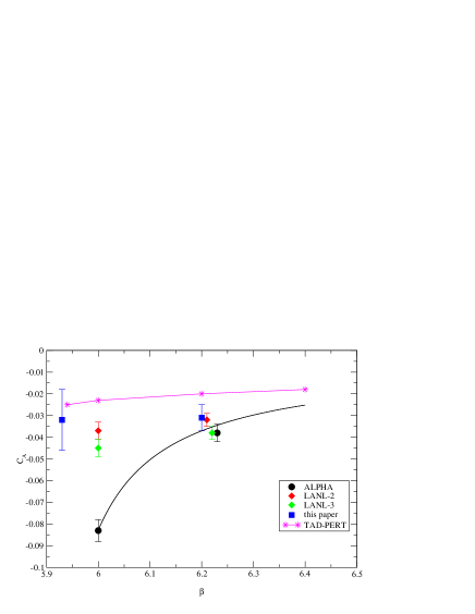
FIG. 1.: $C_{A}$ extracted by various groups. The 1-loop tadpole-improved values for $c_{A}$ were calculated using $\alpha_{P}(1/a)$. Also shown as a black line is the Pade expansion of the ALPHA results [5]. The ALPHA and LANL results at $\beta=6.2$ are offset for clarity. LANL-3 and LANL-2 refer to the results of the LANL group using standard $O(a^{2})$ derivatives (equation 15) and modified $O(a^{2})$ derivatives [3] respectively.

FIG. 2.: $m(t)$ as a function of timeslice for $\beta=5.93$, $\kappa_{l}=0.1327$ and $LL$ smearing. The dotted line indicates a fit to a constant.

FIG. 3.: The fractional contribution of the ground state (squares) and the sum of the ground state and first excited state (diamonds) to the $C_{PA_{4}}$ and $C_{PP}$, $LL$ and $FL$ correlators for $\beta=5.93$ and $\kappa=0.1327$.

FIG. 4.: The values of $c_{A}$ obtained using the LANL method at $\beta=5.93$ and $\kappa_{l}=0.1327$ as a function of $t_{ex}$ used in the fit. $\delta$ indicates the type of lattice derivatives used.

FIG. 5.: $m(t)=r(t)$, $s(t)$ and $m_{imp}(t)=r(t)+ac_{A}s(t)$ as a function of timeslice at $\beta=5.93$ and $\kappa_{l}=0.1327$ for $LL$ correlators. The dotted lines indicate the values for $2am_{PCAC}$ obtained from fitting the results to a constant The dashed lines indicate the value of $2am_{PCAC}^{imp}$ obtained from the fit for $c_{A}$, where the fitting range $7-12$ was used to extract $c_{A}$ for $O(a^{2})$ derivatives (bursts) and $6-12$ for $O(a^{4})$ (squares). These data points also include the statistical error of $c_{A}$.

FIG. 6.: The values of $c_{A}$ obtained from chiral extrapolation in $aM_{PS}^{2}$ at $\beta=5.93$ as a function of $t_{ex}$ used in the LANL fit. The dashed points indicate that an uncorrelated chiral extrapolation was performed.

FIG. 7.: $c_{A}$ as a function of $aM_{PS}^{2}$ at $\beta=5.93$ for $LL$ correlators. The fitting range $6-12$ was used for $O(a^{4})$ derivatives (squares) and $7-12$ for $O(a^{2})$ derivatives (diamonds).

(a)                                                                                      (b)

(c)                                                                                      (d)

FIG. 8.: (a) $c_{A}$ as a function of $t_{ex}$ for $\beta=6.0$ and $\kappa_{l}=0.13344$ with $t_{gs}=12$. $O(a^{4})$ improved derivatives have been used. We found that the $Q$s for the LANL fits were higher than those obtained at $\beta=5.93$. (b) the same as in (a) but with $t_{gs}=16$. (c) $c_{A}$ in the chiral limit from $t_{gs}=12$. (d) $c_{A}(\kappa_{c})$ from $t_{gs}=16$.

(a)                                                                                      (b)

FIG. 9.: (a) $c_{A}$ as a function of $t_{ex}$ for $\beta=6.2$ and $\kappa=0.13460$ with $t_{gs}=16$. $O(a^{4})$ improved derivatives have been used. (b) $c_{A}$ in the chiral limit.

FIG. 10.: The ground state masses of the pseudoscalar meson as a function of $t_{min}$ for the heaviest mesons at $\beta=5.93$ and $6.0$. $C_{PA_{4}}^{FL}$, $C_{PP}^{FL}$, $C_{PP}^{FF}$, $C_{PA_{4}}^{LL}$ and $C_{PP}^{LL}$ were fitted simultaneously, using a fit function including ground ($n=1$) and radially excited states ($n=2,3$). The solid data points indicate fits for which $Q>0.1$. For the dashed results $Q>0.01$ but $<0.1$. The star indicates the final value of $t_{min}$ chosen. We found this fitting range to be adequate for all $\kappa$ combinations.

FIG. 11.: The ground state masses of the pseudoscalar meson as a function of $t_{min}$ for the heaviest and lightest meson at $\beta=6.2$. $C_{PA_{4}}^{FL}$, $C_{PP}^{FL}$ and $C_{PP}^{FF}$ were fitted simultaneously, using a fit function including the ground state. The solid data points indicate fits for which $Q>0.1$. For the dashed results $Q>0.01$ but $<0.1$. The star indicates the final value of $t_{min}$ chosen. We used this fitting range for all $\kappa$ combinations.

(a)                                                                                      (b)

(c)                                                                                      (d)

FIG. 12.: $r_{0}^{2}M_{PS}^{2}$ vs $r_{0}m_{PCAC}^{imp}$. (a) using $c_{A}$ as determined in this paper and (b) as determined by the ALPHA collaboration.(c) shows the quantity $y$ as a function of $x$ as defined in equations D2 and D3 for all 3 $\beta$ values. (d) presents the results for $\beta=5.93$ only. Note that in (c) and (d) $m_{PCAC}^{(0)}$ has been used.

(a)                                                                                      (b)

(c)

FIG. 13.: $r_{0}^{2}M_{PS}^{2}$ and $r_{0}m_{PCAC}^{imp}$ vs $r_{0}m_{\kappa}$. $m_{\kappa}$ is calculated using $\kappa_{c}$ obtained from the fits shown for each $\beta$ value. In (b) our results for $c_{A}$ are used and in (c) the $c_{A}$ determined by the ALPHA collaboration.

(a)                                                                                      (b)

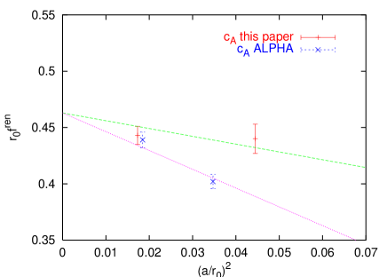
(c)

FIG. 14.: The renormalised pseudoscalar decay constant. (a) $r_{0}f^{ren}$ vs $r_{0}^{2}M_{PS}^{2}$ using the values of $c_{A}$ calculated in this paper. The errors are statistical, and include the statistical error of $c_{A}$. (b) as in (a) using $c_{A}$ from the ALPHA collaboration. Here the errors on $c_{A}$ have been neglected. (c) The scaling of $r_{0}f^{ren}$ for the reference mass $(r_{0}M_{PS})^{2}=3.0$. The dashed line indicates a simultaneous fit to the data sets obtained using our $c_{A}$ values and those from the ALPHA collaboration. The errors include the uncertainties in the coefficients $b_{A}$ and $Z_{A}$. The results at $\beta=6.2$ have been offset slightly for clarity.

(a)                                                                                      (b)

FIG. 15.: Scaling of $r_{0}m^{\overline{MS}}(2GeV)$ for $r^{2}_{0}M_{PS}^{2}=3.0$ (a) obtaining the renormalised quark mass from the bare PCAC quark mass via the renormalisation-group invariant mass (see equation C4) and using our values of $c_{A}$ and those of the ALPHA collaboration. The errors include the uncertainty in $c_{A}$ (for our $c_{A}$ values only) and $Z_{M}$. The dashed line indicates a simultaneous fit to both data sets. (b) As in (a) but calculating $m^{\overline{MS}}$ directly using the 1-loop perturbative results. This is compared and simultaneously fitted to the 1-loop results for the quark mass extracted using $\kappa_{c}$, which is independent of $c_{A}$. The errors include estimates of the perturbative uncertainty in $Z_{A}/Z_{P}$. In both plots the data points have been offset for clarity.

REFERENCES

- [1] K. Symanzik, Nucl. Phys. B226 187 (1983).
- [2] T. Bhattacharya et. al., Phys, Rev. D63 074505 (2001).
- [3] T. Bhattacharya et. al., Phys. Lett. B461 79-88 (1999).
- [4] R. Gupta, Lattice 2001 proceedings.
- [5] ALPHA collaboration, M. Lüscher et. al., Nucl. Phys. B491 323 (1997).
- [6] M. Guagnelli et. al., hep-lat/0009021.
- [7] C. T. H. Davies et. al., Phys. Rev. D56, 2755 (1997).
- [8] UKQCD collaboration, K. Bowler et. al, Phys. Rev. D62 054506 (2000).
- [9] M. Lüscher and P. Weisz, Nucl.Phys.B479:429-458, (1996).
- [10] H. Wittig, private communication.
- [11] J. Garden et. al., Nucl. Phys. B571, 237-256(2000).
- [12] R. G. Edwards et. al, Phys. Rev. Lett. 80, 3448 (1998).
- [13] UKQCD Collaboration, P. Lacock et. al., Phys. Rev. D51 6403 (1995).
- [14] UKQCD Collaboration, C. R. Allton et. al., Phys. Rev. D47 5128 (1993).
- [15] M. Guagnelli et. al., Nucl. Phys. B535:389-402 (1998).
- [16] UKQCD collaboration, C. Allton et. al., hep-lat/0107021.
- [17] M. Lüscher et. al., Nucl. Phys. B491:344-364 (1997).
- [18] G. Martinelli et. al., Phys. Lett. B311, 241 (1993).
- [19] G. Martinelli et. al., Nucl. Phys. B445, 81-108 (1995).
- [20] S. Sint and P Weisz, Nucl.Phys.B502:251-268, (1997).
- [21] S. Capitani et. al., Nucl. Phys. B544, 669-698 (1999).
- [22] Y. Taniguchi and A. Ukawa, Phys. Rev. D58 114503 (1998).
- [23] CP-PACS Collaboration S. Aoki et. al., Phys. Rev. Lett. 84, 238 (2000).
- [24] C. Bernard et. al., Phys. Rev. D64, 054506 (2001).
- [25] W. Bardeen et. al., Phys. Rev. D62, 114505 (2000).
- [26] M. Göckeler et. al., Phys. Rev. D57 5562 (1998).