Exploiting finite-size-effects to simulate full QCD with light quarks—a progress report

Abstract

We present a report on the status of the GRAL project (Going Realistic And Light), which aims at simulating full QCD with two dynamical Wilson quarks below the vector meson decay threshold, $m_{\rm ps}/m_{\rm v}<0.5$, making use of finite-size-scaling techniques.

1 INTRODUCTION

The computer simulation of full QCD in the regime of light quark masses, i.e. below the vector meson decay threshold, $R\equiv m_{\rm ps}/m_{\rm v}<0.5$, represents one of the most interesting and yet long standing goals of lattice QCD. As the algorithms and computer resources of today are still inadequate for directly simulating realistic quark masses without running into severe finite size effects (FSE), GRAL will make a virtue of necessity by performing simulations on sequences of small and medium sized lattices; using finite size scaling techniques we will attempt to extrapolate the results to the infinite volume prior to the chiral and continuum extrapolations. In order to make contact with SESAM and T$\chi$L data we use standard Wilson fermions.

2 FIXING PHYSICAL PARAMETERS

Seeking to simulate QCD with light quarks our first task is to determine an operating point ($\beta^{\rm op}$, $\kappa^{\rm op}$) in parameter space with $R^{\rm op}<R_{d}=0.5$. In order to render simulations at this point feasible we specify $N_{s}=16$ as the maximal spatial extent of a series of lattices employed. With the number of lattice points in temporal direction held fixed at $N_{t}=32$, the computational cost for $N_{s}=16$ thus sets an upper bound for the costs of subsequent simulations on smaller lattices.

To be specific, we require the simulation with $N_{s}^{\rm op}=16$ at $(\beta^{\rm op},\kappa^{\rm op})$ to yield meson masses with $R^{\rm op}=0.4$ and a FSE of $z^{\rm op}=0.2$. This particular value for the finite size parameter $z\equiv 1/(am_{\rm ps}N_{s})$ has been chosen in view of a recent SESAM/T$\chi$L quark mass analysis [1], where $z\approx 0.2$ was found to mark the onset of significant FSE’s in the spectrum.

In summary, the envisaged properties of our target point on a $16^{3}\times 32$-lattice are as follows:

$$\begin{array}[]{ccccccc}\hline\cr\lx@intercol\hfil\rule[-5.69054pt]{0.0pt}{17.07164pt}\frac{m_{\rm ps}}{m_{\rm v}}\hfil\lx@intercol&\lx@intercol\hfil\rule[-5.69054pt]{0.0pt}{17.07164pt}z\hfil\lx@intercol&\lx@intercol\hfil\rule[-5.69054pt]{0.0pt}{17.07164pt}\xi_{\rm ps}\hfil\lx@intercol&\lx@intercol\hfil\rule[-5.69054pt]{0.0pt}{17.07164pt}am_{\rm ps}\hfil\lx@intercol&\lx@intercol\hfil\rule[-5.69054pt]{0.0pt}{17.07164pt}am_{\rm v}\hfil\lx@intercol&\lx@intercol\hfil\rule[-5.69054pt]{0.0pt}{17.07164pt}a[{\rm fm}]\hfil\lx@intercol&\lx@intercol\hfil\rule[-5.69054pt]{0.0pt}{17.07164pt}L\ [{\rm fm}]\hfil\lx@intercol\\ \hline\cr 0.4&0.2&3.2&0.31&0.78&0.116&1.86\\ \hline\cr\end{array}$$

The lattice spacing $a\equiv a_{\rho}^{l}$ has been estimated on the basis of the SESAM and T$\chi$L data at $\beta=5.6$ and $5.5$. Obviously, the price for sticking to $N_{s}=16$ is a fairly coarse lattice. However, according to the scaling formulae in [2], we expect a total cost of approximately $0.2\;\mathrm{TFlop/s}\cdot\mathrm{h}$ to produce 100 statistically independent gauge field configurations at $(\beta^{\rm op},\kappa^{\rm op})$, which is feasible.

3 SEARCHING THE TARGET POINT

On the search for the bare run parameters $(\beta^{\rm op},\kappa^{\rm op})$ we let ourselves be guided by a heuristic consideration. From the known lattice spacings $a=0.095\;\mathrm{fm}$ at $\beta=5.5$ and $0.078\;\mathrm{fm}$ at $5.6$, we deduce an estimate for $\beta^{\rm op}$ from the renormalization group $\beta$-function. Assuming that we are in the scaling regime we get $\partial\beta/\partial\ln a\approx-0.46$, which leads us to expect that the presumed lattice spacing of $a=0.116\;\mathrm{fm}$ at the target point will be attained at $\beta^{\rm op}\approx 5.4$.

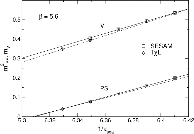
Figure 1: Chiral extrapolation of $m_{\rm v}$ and $m_{\rm ps}^{2}$ for $\beta=5.6$.

With this in mind we turn to the SESAM/T$\chi$L spectral data. The solid lines in fig. 1 represent linear fits to the $m_{\rm v}$ and $m_{\rm ps}^{2}$ data at $\beta=5.6$ with $N_{s}=16$. The dashed lines result from separate fits to the T$\chi$L data with $N_{s}=24$. We use these fits (and corresponding ones for $\beta=5.5$) to establish functional dependencies of $R$ and $z$ on $1/\kappa$, as shown in fig. 2.

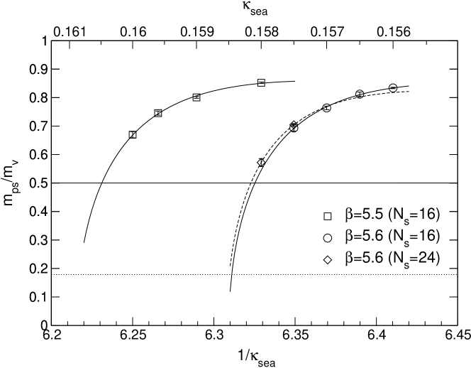
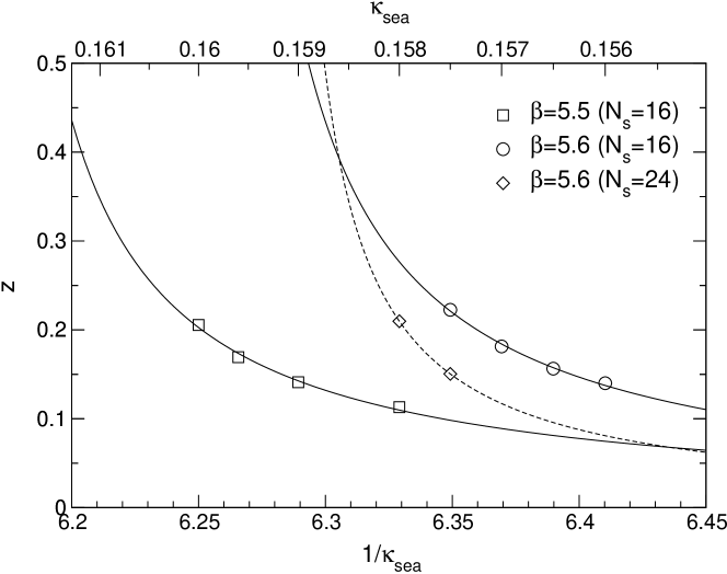
Figure 2: $R$ (a) and $z$ (b) as functions of $1/\kappa$.

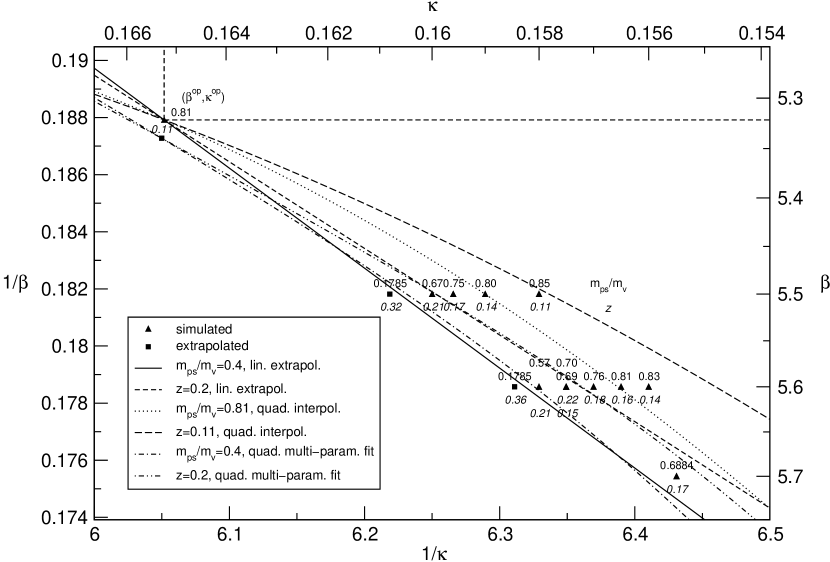
Figure 3: Lines of constant $m_{\rm ps}/m_{\rm v}$ and $z$ in the $\beta$-$\kappa$ plane.

We are now in the position to guesstimate the operating point by direct extrapolation in the $\beta$-$\kappa$ plane. Setting out from the functions of fig. 2 we use a linear and a quadratic ansatz to construct curves of constant $R$ and $z$ in that plane, displayed in fig. 3. The intersection of the straight lines for $R\equiv 0.4$ (solid) and $z\equiv 0.2$ (dashed) in the $\beta$-$\kappa$ plane delivers with $(\beta^{\rm op},\kappa^{\rm op})=(5.32,0.1652)$ a first estimate for the operating point. Although $\beta^{\rm op}$ comes out close to the estimate from the $\beta$-function, this result is not to be taken too seriously, as preliminary results of a simulation performed with these action parameters give $R(\beta^{\rm op},\kappa^{\rm op})=0.8$ and $z(\beta^{\rm op},\kappa^{\rm op})=0.1$, which is off the expectation by a factor of two in both cases. In order to illustrate qualitatively the behavior of $R(\beta,\kappa)$, the long-dashed curve shows a quadratic interpolation between $(\beta^{\rm op},\kappa^{\rm op})$ (having $R=0.8$) and the points with the same $R$ at $\beta=5.5$ and $5.6$. (The dotted curve shows the same for $z(\beta,\kappa)$.)

A two-dimensional quadratic fit of all available (simulated and extrapolated) $R(\beta,\kappa)$ and $z(\beta,\kappa)$, respectively, to functions of the form $f(\beta,\kappa)=c_{0}+c_{1}\beta+c_{2}\kappa+c_{3}\beta^{2}+c_{4}\kappa^{2}+c_{5}\beta\kappa$ leads to the coordinates $(\beta^{\rm op},\kappa^{\rm op})=(5.34,0.1653)$. The dot-dashed curves in fig. 3 show the resulting $\beta(\kappa)$ for $R\equiv 0.4$ and $z\equiv 0.2$. As this second guess for $(\beta^{\rm op},\kappa^{\rm op})$ deviates only little from the first one we are still running at $\beta=5.32$, but with increased values of $\kappa$. Production is carried out on APEmille at DESY Zeuthen.

4 SIMULATION PLAN

For the smaller lattices ($N_{s}<16$) we will use the cluster computer ALiCE at the University of Wuppertal. To carry out a chiral extrapolation, we will generate additional ensembles at equal $\beta$, but larger $R$. The step to a larger $\beta$ can be done either by going to $N_{s}=18,20,22$ at $R=0.4$ and $z=0.2$, or by moving on to $z>0.2$, depending on the results at the present simulation point. We are aware of the fact that our operating point may be located far in the strong coupling regime. On the other hand we might possibly take advantage of the increased “$\beta$-shifts” at light sea quark masses. Eventually we want to reach values of $\beta\geq 5.6$.

For the extrapolation to the infinite volume limit we expect a formula of the form $m=m_{\infty}+cL^{-\nu}$ to be applicable [3]. Fig. 4 shows results of Fukugita et al.; the solid lines are fits with $\nu=3$ to their full QCD data.

Figure 4: Extrapolation to infinite volume.

References

- [1] N. Eicker et al., these proceedings
- [2] Th. Lippert, these proceedings
- [3] M. Fukugita, H. Mino, M. Okawa, G. Parisi, A. Ukawa, Phys. Lett. B 294 (1992) 380.