$1/M$ correction to quenched QCD with non-zero baryon density

Abstract

We study the $\kappa^{2}$ corrections to the quenched limit of $\mu>0$ QCD. We use an improved reweighting procedure.

Introduction  In Fig. 1 we sketch tentative features of the QCD phase diagram in the $\kappa,\,\mu,\,T$ space. Since a general description is missing, one may try to concentrate on special situations, such as the “quenched” limit [1] (see below), represented by the thick vertical dashed line at infinite $\mu$ in the $\kappa=0$ plane. For a more physical situation we consider a vertical plane at small but non-zero $\kappa$, then, e.g., a possible transition would appear at $\mu_{c}(\kappa,T)<\infty$. Here we present a first attempt to describe phenomena away from the quenched limit.

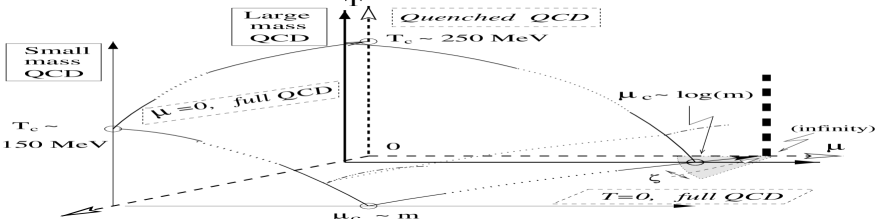
Figure 1: Tentative phase diagram.

Hopping parameter expansion  The QCD grand canonical partition function is (we specify for one flavour of Wilson quarks and neglect constant factors; $U$ are links, $T$ lattice translations):

$${\cal Z}(\beta,\kappa,\mu)=\int[DU]\,{\rm e\,}^{-S_{G}(\beta,\{U\})}{\cal Z}_{F}({{\kappa}},\mu,\{U\}),$$

$${\cal Z}_{F}({{\kappa}},\mu,\{U\})={\rm Det\,}W({{\kappa}},\mu,\{U\}),$$ (1)

$$W=\!\!\!\!\!\! \!\!\!\!1-\kappa\,\sum_{i=1}^{3}\left(\Gamma_{+i}\,U_{i}\,T_{i}+\Gamma_{-i}\,T^{*}_{i}\,U^{*}_{i}\right)$$ (2)

$$\!\!\!\!-\kappa\,\left({\rm e\,}^{\mu}\,\Gamma_{+4}\,U_{4}\,T_{4}+{\rm e\,}^{-\mu}\,\Gamma_{-4}\,T^{*}_{4}\,U^{*}_{4}\right),$$

with $\Gamma_{\pm\mu}=1\pm\gamma_{\mu}$, $2\kappa=\frac{1}{{\tilde{m}}+3+\cosh\mu}=\frac{1}{m+4}$. Here ${\tilde{m}}$ is the naive continuum limit “bare mass”, $m$ the bare mass at $\mu=0$. The analytic expansion in $\kappa$ leads to an expansion in closed loops, the links contributing factors $\kappa$ or $\kappa{\rm e\,}^{\pm\mu}$, see (2):

$$\!\!\!\!{\cal Z}_{F}({{\kappa}},\mu,\{U\})={\rm Det\,}W={\rm exp}({\rm Tr\,}\ln W)$$

$$\!\!\!\!={\rm exp}\left[-\sum_{l=1}^{\infty}\sum_{\left\{{\cal C}_{l}\right\}}\sum_{s=1}^{\infty}~{}{{{(\kappa^{l}f_{{\cal C}_{l}})}^{s}}\over s}\,{\rm Tr\,}_{\rm D,C}{\cal L}_{{\cal C}_{l}}^{s}\right]$$

$$\!\!\!\!=\prod_{l=1}^{\infty}~{}\prod_{\left\{{\cal C}_{l}\right\}}~{}{\rm Det\,}_{\rm D,C}\left(1~{}-~{}{{\kappa}}^{l}f_{{\cal C}_{l}}{\cal L}_{{\cal C}_{l}}\right)$$ (3)

(D, C $=$ Dirac, colour). ${\cal C}_{l}$ are distinguishable, non-exactly-self-repeating closed paths of length $l$, $s$ is the number of times a loop ${\cal L}_{{\cal C}_{l}}$ covers ${\cal C}_{l}$,

$$f_{{\cal C}_{l}}=\left(\epsilon\,{\rm e\,}^{\pm N_{\tau}\mu}\right)^{r}\ {\rm if}\ {\cal C}_{l}=``Polyakov\,\,r\!\!-\!\!path"\!,\!$$ (4)

1 otherwise. A $``Polyakov\ r\!\!-\!\!path"$ closes over the lattice in the $\pm 4$ direction with winding number $r$ and periodic(antiperiodic) b.c. [$\epsilon=+1(-1)$].

Quenched limit at $\mu>0$  In the double limit [2] $\kappa\rightarrow 0,\,\mu\rightarrow\infty$ with $\kappa\,{\rm e\,}^{\mu}\equiv\zeta$ fixed, only straight, positive Polyakov loops ${\cal P}_{\vec{x}}$ are retained:

$${\cal Z}_{F}^{[0]}(C,\left\{U\right\})=\exp\left[-\sum_{\left\{{\vec{x}}\right\}}\sum_{s=1}^{\infty}\!\!~{}{{{(\epsilon C)}^{s}}\over s}~{}{\rm Tr\,}_{\rm C}({\cal P}_{\vec{x}})^{s}\right]$$

$$=\,\prod_{\left\{{\vec{x}}\right\}}~{}{\rm Det\,}_{\rm C}\left(1~{}-~{}\epsilon\,C{\cal P}_{\vec{x}}\right)^{2},\,\,\,\,\,\,C=(2\,\zeta)^{N_{\tau}}$$ (5)

(see [2], and [1, 3] for further studies). $C$ (or $\zeta$) fixes the direction toward the limit - see Fig. 1.

Next order corrections  To disentangle the effects of $\kappa$ and $\mu$ we go to next order in $\kappa$:

$${\cal Z}_{F}^{[2]}({{\kappa}},\mu,\left\{U\right\})={\rm exp}\left\{-2\,\sum_{\left\{{\vec{x}}\right\}}\,\sum_{s=1}^{\infty}\,{{{(\epsilon\,C)}^{s}}\over s}\right.{\times}$$

$$\left.{\rm Tr\,}_{\rm C}\left[({\cal P}_{\vec{x}})^{s}+\kappa^{2}\sum_{r,q,i,t,t^{\prime}}(\epsilon\,C)^{s(r-1)}({\cal P}_{{\vec{x}},i,t,t^{\prime}}^{r,q})^{s}\right]\right\}$$

$$= \!\!\!\!\!\!\!\!{\cal Z}_{F}^{[0]}(C,\left\{U\right\})\times$$ (6)

$$\!\!\!\!\!\!\prod_{{\vec{x}},r,q,i,t,t^{\prime}}{\rm Det\,}_{\rm C}\left(1-(\epsilon\,C)^{r}\,\kappa^{2}\,{\cal P}_{{\vec{x}},{i},t,t^{\prime}}^{r,q}\right)^{2}.$$

For easy bookkeeping we use the temporal gauge $U_{n,4}=1$, except for $U_{({\vec{x}},n_{4}=N_{\tau}),4}\equiv V_{\vec{x}}$: free, and

$${\cal P}_{{\vec{x}},i,t,t^{\prime}}^{r,q}=(V_{\vec{x}})^{r-q}U_{({\vec{x}},t),i}(V_{{\vec{x}}+{\hat{\i}}})^{q}U_{({\vec{x}},t^{\prime}),i}^{*}$$ (7)

with $r>q\geq 0$, $i=\pm 1,\pm 2,\pm 3$, $1\leq t\leq t^{\prime}\leq N_{\tau}$ ($t<t^{\prime}$ for $q=0$). As an approximation to the full theory one may expect (6) to be good in some small region around the vertical limit line and by varying $\mu$ or $T$ we may hope to get information, say, about the phases around $\mu_{c}$ at large mass. Alternatively we may propose (6) as a model by itself. At large $\mu$ and mass it would be an approximation in the above sense at all $T$. At large $T$ it would also be an approximation for any $\mu$, as we recover the “Polyakov loop model” there [4]. We may thus hope that our model retains some features of QCD with full $\kappa$, $\mu$ dependence.

Figure 2: History of weight (above) and density (below), $N_{\tau}=4,\,\beta=5.5,\,\kappa=0.12,\,\mu=0.6267$.

Improving convergence of $\mu>0$ simulations  Since at $\mu>0$ ${\cal Z}_{F}$ is complex, simulations using reweighting methods suffer from a “sign problem”. In this situation one can try to realize the cancellations between contributions in a correlated way. This can be done by identifying appropriate transformations of the configurations and correspondingly separate the measure into symmetric and antisymmetric factors, to be used in the MC generation and reweighting, respectively. In special cases this method can be developed to a solution of the sign problem [5], in our case we may hope to achieve some improvement - see also [6]. The sensitive dependence of ${\cal Z}_{F}$ on the temporal Polyakov loops suggests to use center rotations. This is especially suggestive for our model (5-6), but the method can be applied also to the full problem. We write

$${\cal Z}\!\!\! = \!\!\!\int[DU\,DV]\,{\rm e\,}^{-S_{G}(\{U,V\})}{\cal Z}_{F}(\{U,V\})$$ (8)

$$= \!\!\!\int[DU\,DV]\,{\cal S}(\{U,V\}){\cal T}(\{U,V\})$$

with center-symmetric ${\cal S}(\{U,V\})={\cal S}(\{U,ZV\})$, $Z=\left\{1,{\rm e\,}^{2\pi i/3},{\rm e\,}^{4\pi i/3}\right\}$, and calculate

$$\langle O\rangle=\frac{\langle\sum_{Z}O^{Z}{\cal T}^{Z}\rangle_{\cal S}}{\langle\sum_{Z}{\cal T}^{Z}\rangle_{\cal S}},\ \ X^{Z}=X(\{U,ZV\}).$$ (9)

Here $\langle\cdot\rangle_{\cal S}$ are averages taken with the Boltzmann factor ${\cal S}$. $U$ denote spatial links. We choose

$${\cal S}={\rm e\,}^{-S_{G}}\,\left|\sum_{Z}{\cal Z}_{F}(\{U,ZV\})\right|.$$ (10)

Alternatively, in the approximation of retaining only the $s=r=1$ terms in (6) we can take for ${\cal S}$

$${\rm e\,}^{-S_{G}-2\epsilon C\left|\,\sum_{\left\{{\vec{x}}\right\}}{\rm Tr\,}_{\rm C}\left[{\cal P}_{\vec{x}}\,+\,\kappa^{2}\,\sum_{\pm{i},t,t^{\prime}}{\cal P}_{{\vec{x}},{i},t,t^{\prime}}^{1,0}\right]\right|}.$$ (11)

Note that ${\cal S}$ already includes $\kappa$ and $\mu$. In Fig. 2 we show the convergence of the weight ${\cal T}$ and charge density averages (12) for each $Z$ in (9) and after symmetrization. Note the good convergence in a regime of large cancellations ($C=0.0407$; the weight is only $\sim 3\%$). The symmetrization improves the statistics by a factor 3-10 in the confining phase. In the deconfining phase, whichever sector is chosen by ${\cal S}$ the method automatically captures the right contribution. For the analysis we use $8^{3}4$ and $8^{3}6$ lattices with $\epsilon=-1$, performing $\sim 10^{5}$ heat-bath/over-relaxation/metropolis sweeps with (10) or (11) and $r=1$ (first 20000 sweeps for thermalization). Errors are estimated with a jackknife analysis.

Figure 3: Above: $n_{B}/T^{3}$ vs $C$, various $\kappa$. Below: $n_{B}/T^{3}$ at fixed $C$ and $m_{B}/10$ vs $\kappa^{2}$.

Results  We calculate the baryon number density $n_{B}$ and the “mobility” $m_{B}$ (we introduce this as a normalized measure for the effect of the $\kappa^{2}$ term):

$$\frac{n_{B}}{T^{3}}\!\!\! = \!\!\!\frac{N_{\tau}^{3}}{3N_{\sigma}^{3}}\,({\hat{n}_{0}+\hat{n}_{1}}),\,\,\,\,\,\,m_{B}=\frac{\hat{n}_{1}}{\hat{n}_{0}+\hat{n}_{1}},$$ (12)

$$\hat{n}_{0}\!\!\! = \!\!\!2C\langle\sum_{\vec{x}}{\rm Tr\,}P_{\vec{x}}\rangle,$$ (13)

$$\hat{n}_{1}\!\!\! = \!\!\!2C{\kappa}^{2}\langle\sum_{\vec{x},\pm{i},t,t^{\prime}}{\rm Tr\,}P_{{\vec{x}},{i},t,t^{\prime}}\rangle,$$ (14)

as well as $\langle\left(\sum_{\vec{x}}{\rm Tr\,}P_{\vec{x}}\right)^{3}\rangle$, the spatial and temporal plaquettes and the topological susceptibility. The effect of the $\kappa^{2}$ correction can be observed in Fig. 3. As expected, the mobility depends primarily on $\kappa$, not on $\mu$, and the correction to the density depends linearly on $\kappa^{2}$ and it can be significant. The most important point, however, is that we can now probe the $\kappa$ and $\mu$ directions independently. The question of phase transitions is investigated in Fig. 4, both along the $T$ and along the $\mu$ direction. We observe the installation of the deconfining regime with increasing $T$ (the temporal Polyakov loop is non-zero in the confining phase due to the fermions). Also, a signal for a transition in $\mu$ is seen, especially at small temperature. We cannot say, however, from these preliminary results whether these are genuine phase transitions or mere crossovers. The further development implies a more detailed analysis.

Figure 4: Above: $n_{B}/T^{3}$ and Polyakov loop vs $\beta$. Below: $n_{B}/T^{3}$ vs $\mu$.

Acknowledgments: We are indebted to M. Alford, J. Berges and C. Wetterich for discussions.

References

• [1] F. Karsch, hep-lat/0106019.
• [2] I. Bender et al., Nucl. Phys. Proc. Suppl.  26 (1992) 323.
• [3] T. Blum et al., Phys. Rev. Lett.  76 (1996) 1019; J. Engels et al., Nucl. Phys. B558 (1999) 307; A. Yamaguchi, Latt’01.
• [4] F. Green and F. Karsch, Nucl. Phys. B238 (1984) 297.
• [5] M. Alford et al., Nucl. Phys. B602 (2001) 61.
• [6] P. de Forcrand and V. Laliena, Nucl. Phys. Proc. Suppl.  83 (2000) 372.