Re ${A_{0}}$ and Re ${A_{2}}$ from Quenched Lattice QCD

Abstract

We have used domain wall fermions to calculate $K\rightarrow\pi$ and $K\rightarrow 0$ matrix elements which can be used to study the $\Delta I=1/2$ rule for K decays in the Standard Model. Nonlinearities in the $\Delta I=3/2$ matrix elements due to chiral logarithms are explored and the subtractions needed for the $\Delta I=1/2$ matrix elements are discussed. Using renormalization factors calculated using non-perturbative renormalization then yields values for real $A_{0}$ and $A_{2}$. We present the details of our quenched $16^{3}\times 32\times 16$, $\beta=6.0$, $M_{5}=1.8$ simulation, where a previous calculation showed that the finite $L_{s}$ chiral symmetry breaking effects are small ($m_{\rm res}\approx 4\rm MeV$).

1 INTRODUCTION

At energies below the electroweak scale the weak interactions are described by local four-fermi operators multiplied by effective coupling constants, the Wilson coefficients. The formal framework to achieve this is the operator product expansion (OPE) which allows one to separate the calculation of a physical amplitude into two distinct parts: the short distance (perturbative) calculation of the Wilson coefficients and the long distance (generally non-perturbative) calculation of the hadronic matrix elements of the operators $Q_{i}$. We calculate on the lattice $K\rightarrow\pi$ and $K\rightarrow 0$. This allows us to calculate the low energy constants in chiral perturbation [1] which, after incorporating the non-perturbative renormalization factors are then translated into $K\rightarrow\pi\pi$ matrix elements. The CP-PACS collaboration has also presented a very similar calculation at this meeting [2].

2 DETAILS OF THE SIMULATIONS

We have used the Wilson gauge action, quenched, at $\beta=6.0$ on a $16^{3}\times 32$ lattice which corresponds to an inverse lattice spacing $a^{-1}=1.922\,{\rm GeV}$. The domain wall fermion height $M_{5}=1.8$ and fifth dimension $L_{s}=16$ give a residual symmetry breaking $m_{\rm res}=0.00124\;\approx 4\,{\rm MeV}$ [3]; 400 configurations separated by 10000 heat-bath sweeps were used in this analysis. $K\rightarrow\pi$ matrix elements were calculated in the $SU(3)_{\rm flavor}$ limit for 5 light quark masses $m_{f}=0.01,0.02,0.03,0.04,0.05$. Since the $K\rightarrow 0$ matrix elements vanish in the $SU(3)$ limit these matrix elements were calculated with non-degenerate quark propagators for 10 mass combinations subject to the constraint $m_{s}-m_{d}=0.01,0.02,0.03,0.04$. We have also calculated the so called eye diagrams with an active charm quark for $m_{f}=0.1,0.2,0.3,0.4$ ( the physical charm quark is around 0.5). However, the analysis for charm-in is still in progress; in this presentation we concentrate on the case with 3-active flavors wherein charm is integrated out assuming it is very heavy. The calculation took about 4 months on 800 Gflops (peak). Quark propagators were calculated using the conjugate gradient method with a stopping residual of $10^{-8}$ with periodic and anti-periodic boundary conditions which amounts to doubling the lattice size in time direction. The two wall source propagators at $t_{K}=5$ and $t_{\pi}=27$ were fixed to Coulomb gauge. For eye diagrams we employed random wall sources spread over time slices $t=14-17$ with 2 hits per configuration. Dividing the three-point correlation functions by the wall-wall pseudoscalar-pseudoscalar correlation function yields the desired matrix elements up to a factor of $2m_{\pi}$ which is determined from a covariant fit to the wall-point two-point function in the range $t=12-20$ for each mass.

3 CALCULATION OF LOW ENERGY CONSTANTS

Since our results unambiguously show that Re$A_{0}$ and Re$A_{2}$ come essentially from the current-current operators (recall these have the largest Wilson coefficients) we will concentrate on these operators from now on. Quenched chiral perturbation theory predicts

$$m_{\pi}^{2}=a_{\pi}(m_{f}+m_{\rm res})\left[1-\delta\ln\left(\frac{a_{\pi}(m_{f}+m_{\rm res})}{\Lambda_{Q\chi pt}^{2}}\right)\right]$$

We find a quenched chiral logarithm coefficient $\delta=0.05(2)$ which has a negligible contribution in our matrix element calculation. Unlike the quenched chiral logarithms, the conventional logarithms coming from quenched chiral perturbation theory induce large corrections to the $\Delta I=3/2$ $K\rightarrow\pi$ matrix element as can be seen in Figure 1. We fit these amplitudes to [4]

$$b_{1}^{(27,1)}m_{M}^{2}[1-(\delta+\frac{6m_{M}^{2}}{(4\pi f)^{2}})\ln(\frac{m_{M}^{2}}{\Lambda^{2}})]+b_{2}^{(27,1)}m_{M}^{4}$$

where $m_{M}^{2}=a_{\pi}(m_{f}+m_{res})$, $f=137\,{\rm MeV}$, $\Lambda=1\,{\rm GeV}$. The conventional chiral logarithm $m_{M}^{2}\ln(m_{M}^{2}/\Lambda^{2})$ is almost linear over the mass range we have used so the fitting routine cannot distinguish this term from the linear term if we leave the coefficient of the logarithm as a free parameter. Since the large coefficient -6 of the logarithm makes the contribution of this term comparable to the contribution of the linear term omitting this term would change $b_{1}^{(27,1)}$ by almost a factor of two. The quenched chiral log contribution is very small.

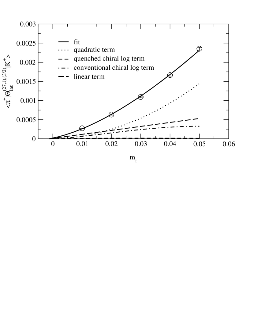
Figure 1: The matrix element $\langle\pi^{+}|\Theta_{lat}^{(27,1)}|K^{+}\rangle$.

$\Delta I=1/2$ $K\rightarrow\pi$ matrix elements mix with $\bar{s}d$ with a power divergent coefficient $\sim(m_{s}+m_{d})/a^{2}$. We define a subtracted matrix element $\langle\pi^{+}|Q_{i}^{(8,1)}|K^{+}\rangle_{sub}$ by

$$\langle\pi^{+}|Q_{i}^{(8,1)}|K^{+}\rangle+\eta_{i}(m_{s}+m_{d})\langle\pi^{+}|\bar{s}d|K^{+}\rangle$$

where $\eta_{i}$ is obtained from a linear fit to $\frac{\langle 0|Q_{i}|K\rangle}{\langle 0|\bar{s}\gamma^{5}d|K\rangle}$. For an explanation of this subtraction of the power divergence we refer the reader to [5]. The quenched chiral perturbation theory corrections to $\langle\pi^{+}|Q_{i}^{1/2}|K^{+}\rangle_{sub}$ are not known. As can be seen in Figure 2 our data is consistent with a linear fit $c_{0,i}+c_{1,i}m_{f}$ with the slope $c_{1,i}$ determining the low energy constants $\alpha_{i}^{1/2}$ and the intercept $c_{0,i}$ arising from residual chiral symmetry breaking.

Figure 2: The matrix element $\langle\pi^{+}|Q_{i}^{1/2}|K^{+}\rangle_{sub}$

4 Re ${A_{0}}$ AND Re ${A_{2}}$

We use chiral perturbation theory to compute the lattice $K\rightarrow\pi\pi$ matrix elements. Using non-perturbative Z factors we obtain the continuum matrix elements which are then multiplied by Wilson coefficients to yield the physical amplitudes. We present an extrapolation to the Kaon mass scale to lowest order in chiral perturbation theory and a second extrapolation which includes one loop logarithmic effects. We multiply the pseudoscalar masses by $\xi$ so that for $\xi\rightarrow 0$ the chiral perturbation theory extrapolation is increasingly accurate but we need the extrapolation at $\xi=1$, the physical point. In figure 3 we present Re${A_{0}}$ and Re${A_{2}}$ as a function of the parameter $\xi$. The chiral logarithm correction for Re${A_{0}}$ is large (about $40\%$). In addition one expects a large correction (not included here) coming from the tree level $O(p^{4})$ terms necessary to cancel the dependence on the chiral perturbation theory scale $\Lambda_{\chi PT}$.

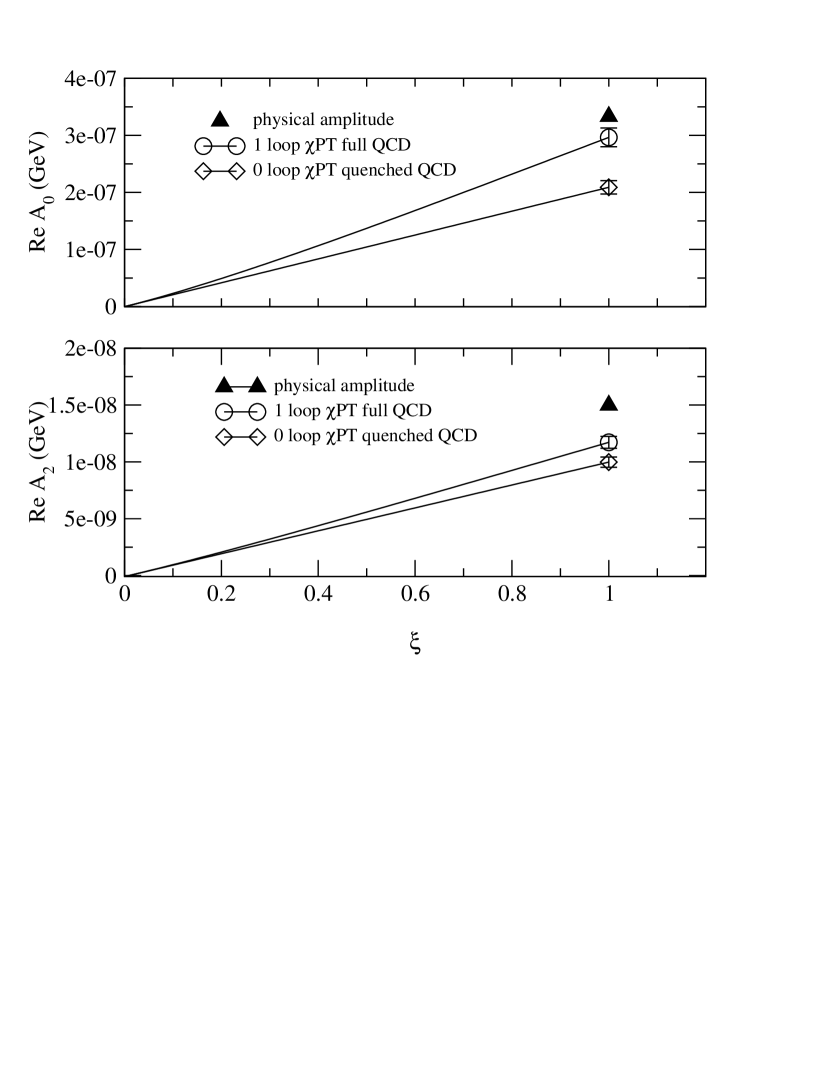
Figure 3: Re${A_{0}}$ and Re${A_{2}}$ as a function of $\xi$

If the Z factors and the Wilson coefficients were calculated to all orders in perturbation theory the physical amplitudes that we calculate would not depend on the scale $\mu$ where the transition between the lattice and the continuum operators is made. To a good approximation this is what we find, even though at $\mu=1.51\,{\rm GeV}$ one expects non-perturbative effects in the Z factors and at $\mu=3.02\,{\rm GeV}$ the discretization errors may be large. In Figure 4 we present the ratio Re${A_{0}}$/Re${A_{2}}$, the so called $\Delta I=1/2$ rule which shows a large enhancement in the $I=0$ channel in accord with experiment (note, the chiral logarithm corrections largely cancel in the ratio so a large enhancement is seen for both extrapolation choices). The residual scale dependence in the physical amplitudes is slight (see Figure 4).

Figure 4: Re${A_{0}}$ and Re${A_{2}}$ obtained using 1-loop logarithmic corrections vs. the matching scale $\mu$; the dotted lines show the experimental results.

5 CONCLUSIONS

In conclusion, Re${A_{0}}$, Re${A_{2}}$ and especially the ratio Re${A_{0}}$/Re${A_{2}}$ were found reasonably close to the experimental values. We see this as an important success of the lattice method. However there were a number of major approximations in our calculation, the hardest to quantify is the use of quenched QCD. Also the chiral logarithms in quenched $K\rightarrow\pi$, $\Delta I=1/2$ are not known and we have included only the logarithmic portion of the next-to-leading-order, 1-loop corrections in $K\rightarrow\pi\pi$ extrapolations.

References

- [1] C. Bernard, et. al., Phys. Rev. D32 (1985) 2343.
- [2] J. Noaki, et. al., hep-lat/0108013, J. Noaki, these proceedings.
- [3] T. Blum, et. al., hep-lat/0007038
- [4] M. Golterman and E. Pallante, JHEP 08, 023 (2000), hep-lat/0006029.
- [5] T. Blum, et. al. (RBC), hep-lat/0110075, R. Mawhinney, these proceedings.
- [6] J. Bijnens, Phys. Lett. B 152 (1985) 226.