Direct Laplacian Center Gauge

Abstract:

We introduce a variation of direct maximal center gauge fixing: the “direct Laplacian” center gauge. The new procedure overcomes certain shortcomings of maximal center gauge, associated with Gribov copies, that were pointed out by Bornyakov et al. in hep-lat/0009035.

1 Introduction

Center projection in direct maximal center gauge is a procedure used to locate center vortices in lattice gauge field configurations. Results obtained from this procedure, which tend to support the center vortex theory of confinement, have been reported in many articles over the past several years. Last year, however, an alarming negative result was reported by Bornyakov, Komarov, and Polikarpov (BKP) in ref. [1]. Recall that direct maximal center gauge fixing is defined by the gauge transformation $g$ which maximizes the sum

$$R=\sum_{x,\mu}\mbox{Tr}_{A}[{}^{g}U_{\mu}(x)]$$ (1)

where $\mbox{Tr}_{A}$ indicates the trace in the adjoint representation, and ${}^{g}U_{\mu}(x)$ is the gauge-transformed lattice configuration. This prescription is simply Landau gauge fixing in the adjoint representation. There is no known method for finding the global maximum of $R$, but most previous work has used the over-relaxation scheme of ref. [2] to find local maxima (Gribov copies). The string tension that can be attributed to vortices, which are located using this scheme, agrees quite well with the asymptotic string tension of the full lattice configuration. This agreement is known as “center dominance,” and is crucial to the argument that center vortices account for the entire asymptotic string tension. In their work last year, BKP used an improved center gauge-fixing scheme based on simulated annealing, and obtained Gribov copies with consistently larger values of $R$ than those obtained by over-relaxation method. The discouraging outcome of this improved gauge-fixing procedure is that center dominance is much less evident: the center projected SU(2) string tension at $\beta=2.5$ is some $30\%$ lower than than the full asymptotic string tension.

In this article we explain the origin of the difficulty found by BKP, and then propose and test a method which overcomes that difficulty. The realization that direct maximal center gauge must fail in the continuum limit is actually due to Engelhardt and Reinhardt in ref. [3], whose work predates the numerical results of BKP in ref. [1]. We have previously elaborated on the Engelhardt-Reinhardt reasoning in ref. [4]; the salient points will be reviewed in section 2 below. In brief, these authors pointed out that direct maximal center gauge can be understood as a best fit to a given lattice gauge field by a thin vortex configuration. Since the field strength of a thin vortex is highly singular, the fit must fail badly near the middle of the vortex. In the continuum limit, the bad fit to the gauge field in the vortex interior would overwhelm the good fit in the exterior region. As a result, in the continuum limit, the center projection obtained from a global maximum of $R$ may reveal no vortices at all.

Having diagnosed the illness, a cure is proposed in section 3. We work throughout with the SU(2) gauge group, although the analysis generalizes readily to SU(N). The new method calls for maximizing

$$R_{M}=\sum_{x,\mu}\mbox{Tr}[M^{T}(x)U_{A\mu}(x)M(x+\hat{\mu})]$$ (2)

where $U_{A\mu}(x)$ denotes the link variable in the adjoint representation, and where, for SU(2) gauge theory, $M(x)$ is a real-valued $3\times 3$ matrix which satisfies the unitarity constraint only as an average; i.e.

$${1\over{\cal V}}\sum_{x}\sum_{j}M^{T}_{ij}(x)M_{jk}(x)=\delta_{ik}$$ (3)

with ${\cal V}$ the lattice volume. The motivation for relaxing the local unitarity constraint is explained below. The real-valued matrix field $M(x)$ which arrives at a global maximum of $R_{M}$ can be determined uniquely, in terms of the three lowest eigenfunctions of a lattice Laplacian operator. To determine the corresponding gauge transformation, we relax $M(x)$ to the closest SO(3) matrix-valued field $g_{A}(x)$ satisfying a related Laplacian condition. The SO(3) field is mapped to an SU(2) matrix-valued field $g(x)$, which is used to gauge-transform the original lattice configuration. Center projection then determines the vortex locations.

In the end, direct Laplacian center gauge is simply lattice Landau gauge, in the adjoint representation, with a particular choice of Gribov copy (different from the global maximum of $R$). We will motivate this choice in sections 2 and 3. Numerical results obtained from the new procedure, regarding center dominance, vortex density scaling, precocious linearity, and the correlation of vortex locations with the values of Wilson loops, are reported in section 4.

Direct Laplacian center gauge is closely related to the original Laplacian Landau gauge of Vink and Wiese [5], appropriately generalized to the adjoint representation. The main difference is in the mapping from $M(x)$ to $g(x)$. Direct Laplacian gauge also has much in common with the Laplacian center gauge, introduced by Alexandrou et al. [6] and de Forcrand and Pepe [7], in that both gauges require solving the lattice Laplacian eigenvalue problem in the adjoint representation. But the gauges themselves are rather different; they are motivated by different considerations (best fit in one case, gauge-fixing ambiguity in the other), and the numerical results are not the same. These points are further discussed in section 5. Section 6 contains our conclusions.

2 Maximal Center Gauge and its Discontents

We begin from the insight that lattice Landau gauge fixing is precisely equivalent to finding the best fit, to a given lattice gauge field $U_{\mu}(x)$, by a classical vacuum configuration $g(x)g^{\dagger}(x+\hat{\mu})$. The best fit vacuum configuration minimizes the mean square distance on the group manifold between vacuum and gauge field link variables

$$d^{2}_{F} = {1\over 4{\cal V}}\sum_{x,\mu}\mbox{Tr}\left[\left(U_{\mu}(x)-g(x)g^{\dagger}(x+\hat{\mu})\right)\left(U_{\mu}(x)-g(x)g^{\dagger}(x+\hat{\mu})\right)^{\dagger}\right]$$ (4)

$$= {1\over 4{\cal V}}\sum_{x,\mu}2\mbox{Tr}\left[I-g^{\dagger}(x)U_{\mu}(x)g(x+\hat{\mu})\right]$$

Writing

$${}^{g}U_{\mu}(x)=g^{\dagger}(x)U_{\mu}(x)g(x+\hat{\mu})$$ (5)

it is is clear that minimizing (4) is equivalent to maximizing

$$\sum_{x,\mu}\mbox{Tr}[{}^{g}U_{\mu}(x)]$$ (6)

in the fundamental representation, which is just the lattice Landau gauge.

Generalizing the above idea slightly, suppose we are interested in finding the best fit of $U_{\mu}(x)$ by a thin center vortex configuration, which has the form

$$V_{\mu}(x)=g(x)Z_{\mu}(x)g^{\dagger}(x+\hat{\mu})$$ (7)

where the $Z_{\mu}(x)=\pm 1$ are $Z_{2}$ link variables. Since the adjoint representation is blind to center elements, we may proceed in the following way: First find the vacuum configuration $g(x)g^{\dagger}(x+\hat{\mu})$ which is a best fit to $U_{\mu}(x)$ in the adjoint representation, i.e. which minimizes

$$d^{2}_{A} = {1\over 4{\cal V}}\sum_{x,\mu}\mbox{Tr}_{A}\left[\left(U_{\mu}(x)-g(x)g^{\dagger}(x+\hat{\mu})\right)\left(U_{\mu}(x)-g(x)g^{\dagger}(x+\hat{\mu})\right)^{\dagger}\right]$$ (8)

$$= {1\over 4{\cal V}}\sum_{x,\mu}2\mbox{Tr}_{A}\left[I-g^{\dagger}(x)U_{\mu}(x)g(x+\hat{\mu})\right]$$

It is clear that the minimum of $d^{2}_{A}$ is obtained at the maximum of

$$R=\sum_{x,\mu}\mbox{Tr}_{A}[{}^{g}U_{\mu}(x)]$$ (9)

which is, by definition, direct maximal center gauge. Having determined $g(x)$ in this way (up to a residual $Z_{2}$ symmetry), we then want to find the $Z_{\mu}(x)$ such that the thin vortex configuration $V_{\mu}(x)$ is a best fit to $U_{\mu}(x)$. This means minimizing, in the fundamental representation

$$d^{2} = {1\over 4{\cal V}}\sum_{x,\mu}\mbox{Tr}\left[\left(U_{\mu}(x)-g(x)Z_{\mu}(x)g^{\dagger}(x+\hat{\mu})\right)\left(U_{\mu}(x)-g(x)Z_{\mu}(x)g^{\dagger}(x+\hat{\mu})\right)^{\dagger}\right]$$ (10)

$$= {1\over 4{\cal V}}\sum_{x,\mu}2\mbox{Tr}\left[I-Z_{\mu}(x)g^{\dagger}(x)U_{\mu}(x)g(x+\hat{\mu})\right]$$

For fixed $g(x)$, minimization is achieved by setting

$$Z_{\mu}(x)=\mbox{signTr}[{}^{g}U_{\mu}(x)]$$ (11)

which is the center projection prescription. In this way we see that maximal center gauge, plus center projection, is equivalent to finding a “best fit” of the given lattice gauge field $U_{\mu}(x)$ by a thin vortex configuration $V_{\mu}(x)$. This point was first made by Engelhardt and Reinhardt [3] in the context of continuum Yang-Mills theory; here we have transcribed their argument to the lattice.

Unfortunately, it is clear that $V_{\mu}(x)$ must be a very bad fit to $U_{\mu}(x)$ at links belonging to thin vortices (i.e. to the P-plaquettes formed from $Z_{\mu}(x)$). Again, this point was made in ref. [3] in the context of the continuum theory, on the grounds that the field strength of a thin vortex is divergent at the vortex core. We recall that a plaquette $p$ is a P-plaquette iff $Z(p)=-1$ (where $Z(C)$ denotes the product of $Z_{\mu}(x)$ around the contour $C$) and that P-plaquettes belong to P-vortices. This means also that

$$\frac{1}{2}\mbox{Tr}[V(p)]=Z(p)=-1$$ (12)

On the other hand, at large $\beta$ we generally have

$$\frac{1}{2}\mbox{Tr}[U(p)]=1-O\left({1\over\beta}\right)$$ (13)

even at P-plaquettes. Writing link variables $U_{\mu}(x)$ in the form

$$U_{\mu}(x) = g(x)Z_{\mu}(x)e^{iA_{\mu}(x)}g^{\dagger}(x+\hat{\mu})$$

$${}^{g}U_{\mu}(x) = Z_{\mu}(x)e^{iA_{\mu}(x)}$$ (14)

we have

$$\mbox{Tr}[U(p)]=Z(p)\mbox{Tr}[\prod_{links\in p}e^{iA_{\mu}(x)}]$$ (15)

or, in view of (12),(13),

$$\frac{1}{2}\mbox{Tr}[\prod_{links\in p}e^{iA_{\mu}(x)}]\approx-1$$ (16)

But, from eq. (11),

$$\mbox{Tr}\left[e^{iA_{\mu}(x)}\right]\geq 0$$ (17)

on every link. Taken together, the last two equations imply that for some links (at least one) on a P-plaquette, ${}^{g}U_{\mu}(x)$ deviates strongly away from the center elements $\pm I$, and, as a result,

$$\mbox{Tr}_{A}\left[{}^{g}U_{\mu}(x)\right]\ll\mbox{Tr}_{A}\left[I\right]$$ (18)

It follows that the trace of links in the adjoint representation, which is the quantity being maximized in direct maximal center gauge, will be much smaller, on average, in the vicinity of a P-plaquette than on the rest of the lattice.

If we compare the fits to a thermalized lattice that can be obtained from a vacuum configuration (no P-vortices), and from a configuration containing some arrangement of thin vortices on vacuum background, the latter is likely to be a better fit in the lattice region exterior to P-plaquettes, but a much worse fit at the P-plaquettes themselves. In the $\beta\rightarrow\infty$ limit, the bad fit near the P-plaquettes may overwhelm the good fit in the exterior region, particularly if the thermalized lattice contains thick ($\approx$ 1 fm) center vortices which overlap substantially. In that case, the best fit is just a pure-gauge, and the global maximum of $R$ would reveal no vortices at all.

In our opinion, this is the explanation for the discouraging result found by BKP in ref. [1]. Using the simulated annealing method described in that reference, we have found that center projection in direct maximal center gauge has good center dominance properties at strong couplings, but that center dominance degrades as we enter the scaling regime. We have also found that Gribov copies obtained by our original method of over-relaxation arrive at a better fit to the thermalized lattice, as compared to copies generated by simulated annealing, if the computation of $R$ is restricted to plaquettes in the region exterior to P-plaquettes. This is consistent with the idea that the bad fit in the neighborhood of P-plaquettes is the source of the trouble. For details and numerical results regarding this point, we refer the reader to ref. [4].

Having arrived at a diagnosis of the problem, the question is what to do about it. One possibility is simply to continue using the original over-relaxation technique, on the grounds that it provides a better fit to the lattice in the region exterior to P-plaquettes. Unfortunately, if one follows this idea further, gauge-fixing a large number of random copies on the gauge orbit and selecting the copy with the best fit in the exterior region, the string tension comes out too high [4]. Therefore, we cannot recommend the “business-as-usual” approach with much enthusiasm.

Another possibility, suggested by Engelhardt and Reinhardt [3], is to modify $R$ in eq. (1) by introducing a form factor $F$ into the expression, i.e.

$$R^{F}=\sum_{x,\mu}F\Bigl{[}\mbox{Tr}_{A}[{}^{g}U_{\mu}(x)]\Bigr{]}$$ (19)

In particular, one could try the “lower bound” function

$$F[x]=\left\{\begin{array}[]{cl}x&~{}~{}~{}x>\Lambda\cr\Lambda&~{}~{}~{}x\leq\Lambda\end{array}\right.$$ (20)

in an effort to soften the bad fit at P-plaquettes. We have experimented with this form of $F$, but the whole approach is obviously plagued by arbitrariness. With an extra free parameter such as $\Lambda$ (that can be reset at each $\beta$), it is not surprising that one can adjust the projected string tension to the desired result.

Finally, there is the Laplacian center gauge [6] developed by de Forcrand and Pepe [7], which is free of Gribov ambiguities altogether. Our present article is inspired in large part by the de Forcrand-Pepe approach (as well as by the earlier work of Vink and Wiese [5]), but we do have some reservations about the version of Laplacian center gauge discussed in refs. [6, 7]. These reservations concern the lack of scaling of the vortex density, the lack of precocious linearity in the vortex potential, and the prescription for locating vortices from the co-linearity of two Laplacian eigenvectors, which appears to lack the important “vortex-finding property” for thin vortices [8]. This last point, which is relevant to the program of looking for gauge-fixing ambiguities in Laplacian gauges, will be discussed in section 5. In the meantime, we will proceed to the proposal which is main point of this article.

3 Direct Laplacian Center Gauge

To motivate our proposal, we return temporarily to the idea that, since the fit is worst at P-plaquettes, it might be sensible to exclude those contributions from the quality-of-fit function $R$. Specifically, consider introducing a configuration-dependent weighting factor

$$\rho(x;{}^{g}U_{\mu})=\left\{\begin{array}[]{cl}0&~{}~{}~{}x\in\mbox{P-vortex}\cr c&~{}~{}~{}\mbox{otherwise}\end{array}\right.$$ (21)

where center projection of ${}^{g}U_{\mu}$ is used to decide whether or not the site $x$ belongs to a P-plaquette, and $c$ is a constant determined by the constraint

$${1\over{\cal V}}\sum_{x}\rho^{2}(x;{}^{g}U_{\mu})=1$$ (22)

which means that $c^{2}$ is inversely proportional to the lattice volume exterior to P-plaquettes. One then considers

$$R^{\prime}=\sum_{x,\mu}\rho(x;{}^{g}U_{\mu})\rho(x+\hat{\mu};{}^{g}U_{\mu})\mbox{Tr}_{A}[g^{\dagger}(x)U_{\mu}(x)g(x+\hat{\mu})]$$ (23)

which is proportional to the average trace of adjoint links $\mbox{Tr}_{A}[{}^{g}U_{\mu}(x)]$ in the exterior volume, choosing $g(x)$ to maximize this quantity.

However, even the exclusion of all links joined to P-plaquettes is still not good enough in the continuum $\beta\rightarrow\infty$ limit, since there one expects a bad fit also in a finite volume surrounding the P-plaquettes. At low or intermediate values of $\beta$, on the other hand, excluding 100% of the P-plaquette contributions goes too far, because the excluded links are a very substantial fraction of the total lattice volume. The next step, then, is to allow greater flexibility in the weighting factor. This is done by allowing $\rho(x)$ to be a degree of freedom in its own right. Introduce a $3\times 3$ matrix-valued field

$$G_{ij}(x)=\pm\Omega_{ij}(x)\rho(x)$$ (24)

where $\Omega$ is an SO(3) matrix, and consider choosing $\rho,\Omega$ to maximize the quantity

$$R^{\prime\prime}=\sum_{x,\mu}\mbox{Tr}[G^{T}(x)U_{A\mu}(x)G(x+\hat{\mu})]$$ (25)

where $U_{A\mu}(x)$ denotes the link variable in the adjoint representation, and where $\rho(x)$ is a real positive scalar, subject to the constraint

$${1\over{\cal V}}\sum_{x}\rho^{2}(x)=1$$ (26)

This constraint is now simply the requirement that $G(x)$ is orthogonal “on average.” Mapping the SO(3) matrix field $\Omega(x)$ onto an $SU(2)$ matrix field $g(x)$ with, e.g., Tr$[g]>0$, and again defining the lattice field in this new gauge by ${}^{g}U_{\mu}(x)$, one can determine the P-vortex locations from the center projected configuration (11).

Generalizing this stategy one step further, we can replace the positive scalar field $\rho(x)$ by a real, symmetric matrix $P_{ij}(x)$ with positive semidefinite eigenvalues, and write

$$M_{ij}(x)=\pm\Omega_{ik}(x)P_{kj}(x)$$ (27)

(summation is over repeated indices). This is known as the polar decomposition of the matrix $M$. A corollary of the Singular Value Decomposition Theorem [9] is that any real $3\times 3$ matrix $M$ can be decomposed in this way. The idea is then to find the $3\times 3$ matrix-valued field $M(x)$ which maximizes

$$R_{M}=\sum_{x,\mu}\mbox{Tr}[M^{T}(x)U_{A\mu}(x)M(x+\hat{\mu})]$$ (28)

subject to the constraint (which generalizes (26))

$${1\over{\cal V}}\sum_{x}M^{T}(x)M(x)=I$$ (29)

so that $M(x)$ is also orthogonal “on average.”

It is fortunate that the problem we have just posed has both a unique solution, and a standard computational algorithm for arriving at that solution. It is convenient to view the columns of $M(x)$ at any site $x$ as a set of three 3-vectors

$$f^{b}_{a}(x)=M_{ab}(x)~{}~{},~{}~{}\vec{f^{b}}(x)\equiv\left[\begin{array}[]{c}f_{1}^{b}(x)\cr f_{2}^{b}(x)\cr f_{3}^{b}(x)\end{array}\right]$$ (30)

Then in this notation, maximizing $R_{M}$ is equivalent to maximizing

$$S=\sum_{x,\mu}f^{c}_{j}(x)[U_{A\mu}(x)]_{jk}f^{c}_{k}(x+\hat{\mu})+\frac{1}{2}\Lambda_{cd}\sum_{x}\left[f^{c}_{j}(x)f^{d}_{j}(x)-\delta_{cd}\right]$$ (31)

where the $\Lambda$ is a real symmetric matrix of Lagrange multipliers, introduced to enforce the constraint (29). In view of the constraint, the configuration maximizing $S$ also maximizes the expression

$$S^{\prime}=\sum_{x,\mu}\left[f^{c}_{j}(x)[U_{A\mu}(x)]_{jk}f^{c}_{k}(x+\hat{\mu})-f^{c}_{j}(x)f^{c}_{j}(x)\right]+\frac{1}{2}\Lambda_{cd}\sum_{x}\left[f^{c}_{j}(x)f^{d}_{j}(x)-\delta_{cd}\right]$$ (32)

Variation of $S^{\prime}$ wrt $f_{i}^{a}$ then leads to a lattice Laplacian equation

$$\sum_{y}{\cal D}_{ij}(x,y)f^{a}_{j}(y)=\Lambda_{ac}f^{c}_{i}(x)$$ (33)

where

$${\cal D}_{ij}(x,y)=-\sum_{\mu}\left([U_{A\mu}(x)]_{ij}\delta_{y,x+\hat{\mu}}+[U_{A\mu}(x-\hat{\mu})]_{ji}\delta_{y,x-\hat{\mu}}-2\delta_{ij}\delta_{xy}\right).$$ (34)

Because $\Lambda$ is real and symmetric, it can be diagonalized by an orthogonal matrix $O$, i.e.

$$\Lambda = O^{T}\Lambda_{D}O~{}~{},~{}~{}~{}~{}\Lambda_{D}=\mbox{diag}[\lambda_{1},\lambda_{2},\lambda_{3}]$$

$$f^{\prime a}_{i}(x) = O_{ab}f^{b}_{a}(x)$$ (35)

and then the equation satisfied by each $\vec{f^{\prime a}}(x)$ is the Laplacian eigenvalue equation

$$\sum_{y}{\cal D}_{ij}(x,y)f^{\prime a}_{j}(y)=\lambda_{a}f^{\prime a}_{i}(x)~{}~{}~{}~{}\mbox{(no sum over $a$)}$$ (36)

Since ${\cal D}_{ij}(x,y)$ is hermitian, the orthogonality constraint (29) is satisfied by choosing the $\lambda_{a}$ to be three different eigenvalues. Substituting the solutions of (36) back into (32), its not hard to see that $S^{\prime}$ is maximized by choosing eigenvectors corresponding to the three lowest eigenvalues. An efficient numerical algorithm for obtaining the low-lying eigenvectors of a large, sparse matrix (such as our lattice Laplacian) is the Arnoldi method [9]. Conveniently, Fortran routines implementing this method, and easily adaptable to the problem at hand, are freely available [10].

Since $S^{\prime}$ is invariant under the global transformation $f^{a}_{i}(x)\rightarrow f^{\prime a}_{i}(x)=O_{ab}f^{b}_{a}(x)$, we may as well use the solution for the maximum for which $M_{ab}(x)=f^{\prime b}_{a}(x)$. At this point, we have to map the matrix field $M(x)$ onto an SO(3)-valued field $g_{A}(x)$, and this in turn to a corresponding SU(2) gauge transformation $g(x)$. We consider two possibilities:

1. Naive Map:  Choose $g_{A}(x)$ to be the SO(3)-valued field which is closest to $M(x)$, in the sense that

   $$\Bigl{|}\mbox{Tr}[g_{A}(x)M^{T}(x)]\Bigr{|}$$ (37)

   is maximized at each site $x$.

2. Laplacian Map:  Choose $[g_{A}(x)]_{ij}=\tilde{f}_{i}^{j}(x)$ to be the SO(3)-valued field closest to $M(x)$ subject to the constraint that $g_{A}(x)$, like $M(x)$, satisfies a Laplacian equation of the form

   $$\sum_{y}{\cal D}_{ij}(x,y)\tilde{f}^{a}_{j}(y)=\Lambda_{ac}(x)\tilde{f}^{c}_{i}(x)$$ (38)

The “naive” choice is equivalent to the Laplacian Landau gauge of Vink and Wiese [5], generalized to the adjoint representation. It is obtained by first making a singular value decomposition

$$M(x)=U(x)M_{D}(x)V^{T}(x)$$ (39)

with $U,V$ orthogonal matrices and $M_{D}$ a diagonal positive semi-definite matrix. Then make the polar decomposition at each site

$$M(x)=[U(x)V^{T}(x)][V(x)M_{D}(x)V^{T}(x)]\equiv\pm g_{A}(x)P(x)$$ (40)

with $g_{A}(x)$ the SO(3) matrix-valued field

$$g_{A}(x)=\det[U(x)V^{T}(x)]U(x)V^{T}(x)$$ (41)

and $P$ is symmetric and positive semi-definite. Matrix $g_{A}(x)$ is guaranteed to be the SO(3) matrix closest to $M(x)$, in the sense of maximizing the expression (37) [9]. Finally, we map $g_{A}(x)$ at each site onto one of its two possible representatives in the SU(2) group

$$g(x)=\pm{I+\sigma^{a}\sigma^{b}[g_{A}(x)]_{ab}\over 2[1+\mbox{Tr}(g_{A}(x))]}$$ (42)

The choice of sign in (42) is irrelevant, all choices being related by the residual $Z_{2}$ invariance. One can then transform the lattice configuration by $g(x)$ to obtain ${}^{g}U_{\mu}(x)$, and carry out center projection.

The drawback of the “naive” choice is that, while $M(x)$ is a covariantly smooth matrix, whose columns are the low-lying eigenvectors of the lattice Laplacian, this covariant smoothness property is less pronounced in the $g_{A}(x)$ obtained from singular value decomposition. This results in high-frequency “noise” (small scale fluctuations) in the P-vortex surfaces of the projected configuration. We have found the Laplacian mapping to be preferable.

To carry out the Laplacian mapping, we begin with the “naive” mapping, to find the SO(3) matrix field $\Omega(x)$ closest to the real-valued matrix field $M(x)$ obtained from solving the Laplacian eigenvalue equation (36). Then we relax $\Omega(x)$ to the closest solution $g_{A}(x)$ satisfying the generalized Laplacian equation (38). The relaxation is carried out in the following way: We note that the equation (38) is simply the stationarity condition of the action

$$S^{\prime\prime}=\sum_{x,\mu}\left[f^{c}_{j}(x)[U_{A\mu}(x)]_{jk}f^{c}_{k}(x+\hat{\mu})-f^{c}_{j}(x)f^{c}_{j}(x)\right]+\frac{1}{2}\sum_{x}\Lambda_{cd}(x)\left\{f^{c}_{j}(x)f^{d}_{j}(x)-\delta_{cd}\right\}$$ (43)

with $[g_{A}(x)]_{ij}=f_{i}^{j}(x)$ an SO(3) field. With the local Lagrange multiplier field enforcing the SO(3) constraint, a stationary solution of $S^{\prime\prime}$ is easily seen to be a Gribov copy of direct maximal center gauge; local maxima of $S^{\prime\prime}$ are also local maxima of $R$ in eq. (1).

If ${\cal S}[g]\equiv-R$ is regarded as the action of a spin system, with $g_{A}(x)$ the SO(3)-valued field variables, then each Gribov copy can be regarded as a metastable state of system, each with its own “basin of attraction.” The basin of attraction of a metastable state is the volume of all configurations which, when the system is suddenly cooled (or “quenched”), will fall into that metastable state. Over-relaxation is essentially a sudden cooling technique [4], and is therefore perfectly suited to sliding the system “down the hill” of action ${\cal S}$, from the configuration ${}^{\Omega}U_{A\mu}(x)$ to the nearest (or, at least, a nearby) local minimum of ${\cal S}$ (see Fig. 1). The gauge transformation $g(x)$ obtained at this minimum is the Laplacian map of $M(x)$, and the corresponding ${}^{g}U_{\mu}(x)$ is the lattice configuration in direct Laplacian center gauge.

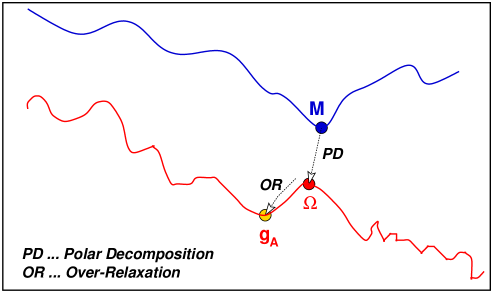
Figure 1: Laplacian mapping of $M(x)$ to a nearby SO(3) matrix-valued field $g_{A}(x)$.

It is interesting that a drawback of the over-relaxation technique, in fixing to maximal center gauge, becomes a virtue in direct Laplacian center gauge. The drawback is that over-relaxation is not good at finding the global minimum of ${\cal S}$, but only takes a given initial state to a nearby local minimum (Gribov copy). In fixing to direct Laplacian gauge, on the other hand, we have taken advantage of the fact that over-relaxation goes to a nearby minimum in order to carry out the Laplacian mapping $M(x)\rightarrow g(x)$.

It may be useful at this stage to summarize the steps of direct Laplacian center gauge fixing:

1. From a thermalized SU(2) lattice, construct the lattice configuration in the adjoint representation

   $$[U_{A\mu}(x)]_{ij}=\frac{1}{2}\mbox{Tr}[\sigma_{i}U_{\mu}(x)\sigma_{j}U^{\dagger}_{\mu}(x)]$$ (44)

2. Solve the eigenvalue problem (36) for the eigenvectors corresponding to the three smallest eigenvalues of the lattice Laplacian operator in the adjoint representation. We have used the ARPACK routines [10] for this purpose. From the eigenvectors $\vec{f^{a}}(x),~{}a=1,2,3$, construct the matrix field $M_{ij}(x)=f_{i}^{j}(x)$.

3. Perform, at each site, the singular value decomposition $M(x)=U(x)M_{D}(x)V^{T}(x)$, and extract the SO(3) matrix-valued field

   $$\Omega(x)=\det[U(x)V^{T}(x)]U(x)V^{T}(x)$$ (45)

4. Map $\Omega$ to an SU(2) matrix-valued field

   $$\omega(x)=\pm{I+\sigma^{a}\sigma^{b}[\Omega(x)]_{ab}\over 2[1+\mbox{Tr}(\Omega(x))]}$$ (46)

   and perform the gauge transformation

   $${}^{\omega}U_{\mu}(x)=\omega^{\dagger}(x)U_{\mu}(x)\omega(x+\hat{\mu})$$ (47)

   The result is to transform the configuration into Laplacian Landau gauge in the adjoint representation.

5. With ${}^{\omega}U_{\mu}(x)$ as the starting point, relax the lattice field to the nearest (or, at least, a nearby) Gribov copy of direct maximal center gauge, using the over-relaxation method described in ref. [2]. The result is the configuration fixed to direct Laplacian center gauge.

To make a long story short, direct Laplacian center gauge in practice is nothing but gauge fixing to adjoint Laplacian Landau gauge, followed by over-relaxation to the nearest Gribov copy of direct maximal center gauge. Both the direct Laplacian and the direct maximal center gauges aim at generating a configuration satisfying locally the adjoint lattice Landau gauge condition. The difference is that the optimal configuration, in maximal center gauge, is generated by a gauge transformation maximizing the $R$ functional, whereas in direct Laplacian center gauge the optimal configuration is generated by a gauge transformation lying closest to a matrix maximizing the $R_{M}$ functional. We hope to have explained, in the previous section, why the global maximum of $R$ is not necessarily the best choice for vortex finding, and to have motivated the alternative choice of Gribov copy corresponding to direct Laplacian center gauge. In the next section, we present results that are obtained from center projection in this gauge.

4 Numerical Results

To test the reasoning of the last section, we have recalculated the vortex observables introduced in our previous work (cf. ref. [12, 2]), with P-vortices located via center projection after fixing the lattice to the new direct Laplacian center gauge.

4.1 Center Dominance and Precocious Linearity

In view of the $\approx 30\%$ breakdown of center dominance in maximal center gauge found by BKP [1], the quantities of most immediate interest are the center-projected Creutz ratios, extracted from $I\times J$ Wilson loops on the center-projected lattice. These are displayed, for $\beta$ in the range $[0.4,2.5]$, in Fig. 2.

Figure 2: Creutz ratios from center-projected lattice configurations, in the direct Laplacian center gauge.

At strong couplings, it is clear from Fig. 2 that $\chi_{cp}(1,1)$ matches up with the analytic prediction, in the full theory, of $\sigma=-\ln(\beta/4)$. At weaker couplings, we display our data for $\beta=2.4$ and $\beta=2.5$ in Figs. 3 and 4. Once again we see the feature of precocious linearity; i.e. the fact that Creutz ratios $\chi_{cp}(R,R)$ at a given $\beta$ vary only slightly with $R$, which means that the center-projected potential is approximately linear starting at $R=2$ lattice spacings. The significance of precocious linearity is that it implies that the center-projected degrees of freedom have isolated the long-range physics, and are not mixed up with ultraviolet fluctuations.

Figure 3: Center projected Creutz ratios at $\beta=2.4$ on various lattice sizes. The horizontal band indicates the full asymptotic string tension and errorbar.

Figure 4: Same as Fig. 3, at $\beta=2.5$.

It is also apparent that the center-projected Creutz ratios are quite close to the asymptotic string tension of the unprojected theory, reported in refs. [13]. This is evidence, at least at these two couplings, of the center dominance property. Our combined data for the range of couplings $\beta=2.2-2.5$ is displayed on a logarithmic plot in Fig. 5. In general $\chi_{cp}(R,R)$ deviates from the full asymptotic string tension by less than 10%.

Figure 5: Combined data, at $\beta=2.2-2.5$, for center-projected Creutz ratios obtained after direct Laplacian center gauge fixing. Horizontal bands indicate the asymptotic string tensions on the unprojected lattice, with the corresponding errorbars.

As another way of displaying both center dominance and precocious linearity, we adopt the usual procedure of assigning a lattice spacing $a(\beta)$ based on the asymptotic string tension in lattice units $\sigma_{Lat}(\beta)$, and the string tension in physical units $\sigma_{phys}=(440~{}\mbox{MeV})^{2}$, i.e.

$$a^{2}(\beta)={\sigma_{Lat}(\beta)\over\sigma_{phys}}$$ (48)

We then display, in Fig. 6, the ratio

$${\chi_{phys}(R,R)\over\sigma_{phys}}={\chi_{cp}(R,R)\over\sigma_{Lat}(\beta)}$$ (49)

as a function of the distance in physical units

$$R_{phys}=Ra(\beta)$$ (50)

for all $\chi_{cp}(R,R)$ data points taken in the range of couplings $\beta=2.3-2.5$. Again we see that the center-projected Creutz ratios and asymptotic string tension are in good agreement (deviation $<10\%$), and there is very little variation in the Creutz ratios with distance.

Figure 6: The ratio of projected Creutz ratios to the full asymptotic string tension, as a function of loop extension in fermis. The data is taken from $\chi_{cp}(R,R)$ at a variety of couplings and lattice sizes.

Precocious linearity can be understood in the following way: Asymptotically, outside the vortex core, a center vortex is a $Z_{N}$ dislocation, which affects the value of large Wilson loops, topologically linked to the vortex, by a center element factor. Assume that P-vortices correctly identify the middle of thick center vortices in lattice configurations. Then center projection in effect collapses the thick ($\approx$ one fermi) core of a vortex to a width of one lattice spacing. This means that the asymptotic effect of thick vortices is obtained, on the projected lattice, at any distance greater than one lattice spacing. If P-plaquettes in a plane are uncorrelated, this leads to a linear potential at short distances on the projected lattice. On the other hand, if precocious linearity is not found on the projected lattice, it means that either the P-vortex surface is very rough, fluctuating on all distance scales, or else that some large fraction of P-plaquettes on the projected lattice belong to P-vortices which are small in extent, and do not percolate. Either case results in some short-range correlations among P-plaquettes in a plane, corresponding to high-frequency phenomena not directly associated with the long-range physics.

4.2 Scaling of the Vortex Density

Denote the total number of plaquettes on the lattice by $N_{T}$, the number of P-plaquettes by $N_{vor}$, and the density $N_{vor}/N_{T}$ of P-plaquettes on the lattice by $p$. We have

$$p = {N_{vor}\over N_{T}}={N_{vor}a^{2}\over N_{T}a^{4}}a^{2}$$

$$= {\mbox{Total Vortex Area}\over 6\times\mbox{Total Volume}}a^{2}$$

$$= {1\over 6}\rho a^{2}$$

where $\rho$ is the center vortex density in physical units. Then, according to asymptotic freedom

$$p={\rho\over 6\Lambda^{2}}\left({6\pi^{2}\over 11}\beta\right)^{102/121}\exp\left[-{6\pi^{2}\over 11}\beta\right]$$ (51)

The average vortex density $p$ can be extracted from the expectation value of center projected plaquettes

$$W_{cp}(1,1) = (1-p)\times(+1)+p\times(-1)=1-2p$$

$$p = \frac{1}{2}(1-W_{cp}(1,1))$$ (52)

Figure 7 is a logarithmic plot of P-vortex density $p$ vs. $\beta$. Errorbars are less than the size of data points. The solid line is the asymptotic freedom prediction (51), with $\sqrt{\rho/6\Lambda^{2}}=50$. We emphasize that the slope of this line represents the proper asymptotic scaling for surface densitites. The slope that would be associated with the scaling of pointlike objects such as instantons, or linelike objects such as monopoles, would be quite different. Note that the apparent scaling of $\chi_{cp}(1,1)=-\ln W_{cp}(1,1)\approx 2p$ in Fig. 2 is just a consequence of the scaling of $p$.

Figure 7: Evidence of asymptotic scaling of the P-vortex surface density. The solid line is the asymptotic freedom prediction (51), with $\sqrt{\rho/6\Lambda^{2}}=50$.

4.3 Vortex-Limited Wilson Loops

A “vortex-limited” Wilson loop $W_{n}(C)$ is defined as the expectation value of an unprojected Wilson loop around some contour $C$, evaluated in the sub-ensemble of configurations in which, on the corresponding center-projected lattice, precisely $n$ P-vortices pierce the minimal area of the loop. If P-vortices on the projected lattice roughly locate the middle of thick center vortices on the unprojected lattice, then in the limit of large loop areas, for the SU(2) gauge group, we expect [2, 12]

$${W_{n}(C)\over W_{0}(C)}\longrightarrow(-1)^{n}$$ (53)

The numerical evidence definitely shows a trend in this direction, as can be seen from our data for $W_{1}/W_{0}$ and $W_{2}/W_{0}$ vs. minimal loop area at $\beta=2.3$, shown in Figs. 8 and 9.

Figure 8: Ratio of the one-vortex to zero-vortex Wilson loops $W_{1}(C)/W_{0}(C)$ vs. loop area, at $\beta=2.3$ on a $16^{4}$ lattice.

Figure 9: Ratio of the two-vortex to zero-vortex Wilson loops $W_{2}(C)/W_{0}(C)$ vs. loop area, at $\beta=2.3$ on a $16^{4}$ lattice.

If P-vortices in the projected configuration locate thick center vortices in the unprojected configurations, and if center vortices are responsible for confinement, then $W_{0}(C)$ should not have an area-law falloff. In Fig. 10 we compare Creutz ratios $\chi_{0}[I,J]$ extracted from rectangular $W_{0}(I,J)$ loops, with the standard Creutz ratios $\chi(I,J)$ from loops evaluated in the full ensemble. As expected, the Creutz ratios of the zero-vortex loops tend to zero with loop area.

Figure 10: Creutz ratios $\chi_{0}(R,R)$ extracted from zero-vortex Wilson loops $W_{0}(I,J)$, as compared to the usual Creutz ratios $\chi(R,R)$ on a $16^{4}$ lattice at $\beta=2.3$.

4.4 Center Vortex Removal

It was suggested by de Forcrand and D’Elia [14] that one could remove center vortices from a given lattice configuration by simply multiplying that configuration by the corresponding center-projected configuration derived in maximal center gauge, i.e.

$$U^{\prime}_{\mu}(x)\equiv Z_{\mu}(x)U_{\mu}(x)$$ (54)

where $Z_{\mu}(x)$ is given by (11). Since the adjoint representation is blind to center elements, it is easy to see that if $g(x)$ is a transformation such that ${}^{g}U_{\mu}(x)$ is in maximal center gauge, then ${}^{g}U^{\prime}_{\mu}(x)$ is also in maximal center gauge. However, there are no P-vortices obtained from center projection of ${}^{g}U^{\prime}_{\mu}$, since

$$Z^{\prime}_{\mu}(x)=\mbox{signTr}[{}^{g}U^{\prime}_{\mu}(x)]=Z^{2}_{\mu}(x)=1$$ (55)

One can therefore say that center vortices, as identified in maximal center gauge, have been removed from the lattice configuration. More precisely, what the modification (54) does is to place a thin vortex (one plaquette thickness) in the middle of each thick center vortex core, whose locations are identified by center projection. At large scales, the effects of the thin and thick vortices on Wilson loops will cancel out. Thus there should be no area law due to vortices in the modified configuration $U^{\prime}_{\mu}$, and the asymptotic string tension should vanish.

The vanishing of string tension in the modified configurations was, in fact, observed in ref. [14], using maximal center gauge fixing by the over-relaxation technique of ref. [2]. Figure 11 is a repeat of the de Forcrand-D’Elia calculation at $\beta=2.3$, using direct Laplacian center gauge rather than direct maximal center gauge, and we find essentially the same result.

Figure 11: Creutz ratios on on the modified lattice, with vortices removed, at $\beta=2.3$. For comparison, we also display the unprojected Creutz ratios (open circles), the center projected Creutz ratios (solid circles), and the asymptotic string tension (horizontal band).

5 Remarks on Gauge-Fixing Ambiguities

The original suggestion of ’t Hooft, in his 1981 article on monopole confinement [15], was to introduce a composite operator in the pure gauge theory transforming like a field in the adjoint representation of the gauge group; for SU(2) gauge theory this operator defines a unitary gauge leaving a residual U(1) symmetry. Monopole worldlines would then be associated with lines along which the gauge transformation is ambiguous. This was the idea which motivated the numerical study of maximal abelian [16] and Laplacian abelian [17] gauges. The idea can be generalized by introducing not one but two composite operators transforming in the adjoint representation. Let us denote these operators, in SU(2) gauge theory, by $\phi_{a}(x)$ and $\eta_{a}(x)$, with color index $a=1,2,3$. One then performs a gauge transformation which takes, e.g., $\phi_{a}$ into the positive color 3 direction at every point, and $\eta_{a}$ to lie in the color 1-3 plane, with $\phi_{3},\eta_{1}>0$. This gauge leaves a remnant $Z_{2}$ symmetry. Gauge-fixing ambiguities occur on surfaces where $\phi(x)$ and $\eta(x)$ are co-linear, and these surfaces are then to be identified with center vortices.

The suggestion of refs. [6, 7] is to choose, for $\phi_{a}(x)$ and $\eta_{a}(x)$, the two lowest lying eigenstates of the covariant lattice Laplacian operator (34) in the adjoint representation; i.e.

$$\phi_{a}(x)\equiv f^{1}_{a}(x)~{}~{},~{}~{}~{}\eta_{a}(x)\equiv f^{2}_{a}(x)$$ (56)

with $\lambda_{1}<\lambda_{2}$ being the two lowest eigenvalues of the Laplacian operator. This is the original version of Laplacian center gauge, which we will refer to as LCG1. Because the procedure involves first fixing to Laplacian abelian gauge, followed by a further gauge fixing which reduces the residual gauge symmetry from U(1) to $Z_{2}$, LCG1 is reminiscent of the indirect maximal center gauge of ref. [12]. As we have pointed out in refs. [19], abelian monopole worldlines in the indirect maximal center gauge lie on center vortex surfaces, and a vortex at fixed time can be viewed as a monopole-antimonopole chain. The same relationship between abelian monopoles and center vortices holds true in LCG1.

Gauge-fixing ambiguities in LCG1 occur when $\phi$ and $\eta$ are co-linear in color space, and it is suggested that these ambiguities can be used to locate vortex surfaces. This approach to vortex finding is certainly quite different from the reasoning outlined in section 3, which is is motivated by a “best fit” procedure. In special cases, notably for a classical vortex solution on an asymmetric lattice with twisted boundary conditions, the co-linearity approach seems to work well [18]. We take note, however, of a simple counter-example: Suppose we insert two vortex sheets “by hand” into a configuration $U_{\mu}(x)$ by the transformation

$$U_{0}(x)\rightarrow U^{\prime}_{0}(x)=\left\{\begin{array}[]{cl}-U_{0}(x)&~{}~{}x_{0}=0~{}\mbox{and}~{}0<x_{1}<L\cr U_{0}(x)&~{}~{}\mbox{otherwise}\end{array}\right.$$ (57)

All other components are unchanged, i.e. $U^{\prime}_{k}(x)=U_{k}(x)$ for $k>0$. This transformation inserts two thin vortex sheets into the lattice, parallel to the $x_{2}-x_{3}$ plane, at $x_{0}=0$. We then ask whether these two vortex sheets will be located by the gauge-fixing ambiguity approach. The answer is clearly no, since the composite Higgs fields $\phi(x)$ and $\eta(x)$ are identical in the original $U_{\mu}(x)$, and in the modified $U^{\prime}_{\mu}(x)$ configurations. This example illustrates the fact that the gauge-ambiguity approach lacks the “vortex-finding property” discussed in ref. [8], which is the ability of a procedure to locate thin vortices inserted at known locations into the lattice. We have argued in ref. [8] that this property should be a necessary (although not sufficient) condition for locating vortices on thermalized lattices.

In practice, on thermalized lattices, vortices are located in LCG1 via center projection, rather than by eigenvector co-linearity [7]. Using center projection to locate vortices, LCG1 recovers the vortex-finding property, for reasons explained in ref. [8]. It also exhibits center dominance of the projected asymptotic string tension. On the other hand, the projected Creutz ratios in LCG1 do not display precocious linearity [7], nor does the vortex surface density scale according to the asymptotic freedom formula [20]. A possible remedy is to first fix the lattice to LCG1, and from there to fix to (direct or indirect) maximal center gauge by an over-relaxation procedure. This latter procedure has, in fact, been tried by Langfeld et al. in ref. [20], with good results for the vortex density. Other vortex observables, discussed in the previous section, have not yet been studied systematically in this approach, which seems to have a great deal in common with the direct Laplacian center gauge we have advocated here.

6 Conclusions

We have tested a procedure for locating center vortices on thermalized lattices, based on the idea of finding the best fit to the thermalized lattice by thin vortex configurations. Our new procedure, which is essentially just a variation of direct maximal center gauge, is designed to soften the inevitable bad fit at vortex cores, due to the singular field strength of thin vortices. The numerical results we have found are promising: Deviations from center dominance are generally less than 10%, P-vortex density scales correctly, and there are the usual strong correlations between P-vortex locations and gauge-invariant observables. Our new method is motivated by an improved understanding of how maximal center gauge works, and it addresses some objections to center gauge fixing that have been raised in the recent literature. We hope it will provide a more solid foundation for further numerical studies.