CERN-TH/2001/157

CPT-2001/P.4211

DESY 01-083

IFIC/01-34

FTUV-010617

LTH 508

Non-perturbative renormalization of the quark condensate in Ginsparg-Wilson regularizations

Pilar Hernández^a,, Karl Jansen^a,b, Laurent Lellouch^c and Hartmut Wittig^a,d,
a CERN, Theory Division,
CH-1211 Geneva 23, Switzerland ^b NIC/DESY Zeuthen
Platanenallee 6, D-15738 Zeuthen, Germany ^c Centre de Physique Théorique, Case 907, CNRS Luminy
F-13288 Marseille Cedex 9, France ^d Division of Theoretical Physics
Department of Mathematical Sciences
University of Liverpool, Liverpool L69 3BX, UK
Abstract

We present a method to compute non-perturbatively the renormalization constant of the scalar density for Ginsparg-Wilson fermions. It relies on chiral symmetry and is based on a matching of renormalization group invariant masses at fixed pseudoscalar meson mass, making use of results previously obtained by the ALPHA Collaboration for O($a$)-improved Wilson fermions. Our approach is quite general and enables the renormalization of scalar and pseudoscalar densities in lattice regularizations that preserve chiral symmetry and of fermion masses in any regularization. As an application we compute the non-perturbative factor which relates the renormalization group invariant quark condensate to its bare counterpart, obtained with overlap fermions at $\beta=5.85$ in the quenched approximation.

June 2001

1 Introduction

The understanding of the low-energy sector of QCD is one of the main goals of lattice simulations of the theory. In particular, the determination of the scalar quark-antiquark condensate associated with the spontaneous breaking of chiral symmetry has been the focus of many recent studies [?,?,?,?,?,?,?]. There are now good prospects for a reliable and precise calculation of this quantity, owing to recent progress in two key areas. The first is the formulation of chiral symmetry on the lattice: it has recently become clear how the familiar consequences of chiral symmetry in the continuum can be preserved at non-zero lattice spacing, by employing lattice Dirac operators that satisfy the Ginsparg-Wilson relation [?] (for reviews of the subject see [?,?,?]). In the context of spontaneous symmetry breaking this makes it possible to extract the quark condensate in a conceptually clean manner through a suitable finite-size scaling analysis [?,?]. Lattice results for the bare, subtracted condensate in infinite volume, $-\Sigma_{\rm sub}$, have already been obtained in this way in the quenched approximation [?,?], using Neuberger’s (or overlap) operator [?] as a realization of the Ginsparg-Wilson relation. In order to present an estimate for the condensate which can be used in phenomenological applications, the bare lattice result must, of course, be renormalized.

The renormalization of matrix elements of composite operators defined on the lattice is the second key area where significant progress has been achieved (for a recent review see [?]). A theoretical framework to address the problem of (in general scale-dependent) renormalization of lattice operators in a completely non-perturbative manner has been developed. The main idea is the introduction of an intermediate renormalization scheme, such as the Regularization Independent (RI) [?] and the Schrödinger functional (SF) [?] schemes. These formalisms have already been used successfully to address the renormalization of quark masses for Wilson [?,?,?], staggered [?] and Domain Wall [?] fermions.

The main subject of this paper is the description of a method to compute non-perturbatively the multiplicative renormalization constant of the scalar density in fermionic regularizations based on the Ginsparg-Wilson relation. Our strategy relies on the matching of renormalization group invariant quark masses at fixed pseudoscalar meson mass, and avoids the direct formulation of intermediate renormalization schemes, such as the SF, for Ginsparg-Wilson fermions. Instead, we make extensive use of the non-perturbative renormalization factor for quark masses, computed by the ALPHA Collaboration for O($a$)-improved Wilson fermions [?]. The method is applicable to the renormalization of scalar and pseudoscalar densities for discretizations of the Dirac operator that preserve chiral symmetry at non-zero lattice spacing, and to the renormalization of quark masses in any fermion discretization. As an example, we determine non-perturbatively the renormalization factor which links the bare scalar condensate obtained using the overlap operator to the renormalization group invariant condensate.

The important issue of quenching will not be adressed here. While the methods described below can be applied without change to the full theory, the calculations discussed are sufficiently costly with present computer and algorithm technology that unquenched calculations are not yet considered. Our main purpose is to demonstrate the feasibility of our strategy, and we restrict ourselves to a single value of the lattice spacing at which the bare subtracted condensate has been computed previously, corresponding to a bare coupling of $\beta=5.85$.

As we will describe below in some detail, our approach to the non-perturbative determination of the renormalization factor for the scalar density requires the calculation of two-point functions in the pseudoscalar channel using overlap fermions. These correlation functions are themselves a rich source of information on low-energy QCD, and allow us to compute the condensate independently from the finite-size scaling analysis of [?]. Furthermore, they serve to calculate the light quark masses as well as the pseudoscalar decay constant in the chiral limit. The detailed discussion of these results is deferred to a companion paper [?].

The outline of the remainder of this paper is as follows. In Section 2 we present our strategy for renormalizing the condensate. A discussion of cutoff effects associated with the use of an intermediate O($a$)-improved Wilson regularization and the intrinsic precision of our method is presented in Section 3. Section 4 contains a description of our simulation results, using the overlap operator as well as O($a$)-improved Wilson fermions at $\beta=5.85$. In Section 5 we present our results for the renormalization factors and compare them to one-loop perturbation theory. Finally, Section 6 contains a summary, including an estimate for the renormalized condensate at $\beta=5.85$. Some details concerning improvement coefficients for O($a$)-improved Wilson fermions are described in Appendix A.

2 Strategy

In this section we describe the renormalization of the scalar condensate for overlap fermions. Our strategy relies on the fact that the renormalization constants for the scalar and pseudoscalar densities are identical and are equal to the inverse of the renormalization factor for fermion masses, as can be shown using the chiral Ward Identities for Ginsparg-Wilson fermions (see, e.g. ref. [?])

$$Z_{\rm P}=Z_{\rm S}=\frac{1}{Z_{\rm m}}.$$ (2.1)

The non-perturbative renormalization of quark masses has been studied extensively on the lattice. In particular, the relation between the renormalization group invariant (RGI) mass and its counterpart in the intermediate SF scheme is known with an accuracy of better than 2% in the continuum limit [?]. Furthermore, the non-perturbative matching between the SF scheme and O($a$)-improved Wilson fermions has been performed for a range of bare couplings [?]. One possible strategy is then to repeat this second step for overlap fermions, by evaluating the normalization condition of ref. [?]. However, the direct implementation of the SF scheme for the overlap operator is not straightforward, due to the inhomogeneous boundary conditions in the time direction, which are incompatible with the Ginsparg-Wilson relation. We have thus devised an alternative strategy, which allows us to exploit the previously obtained non-perturbative relations between quantities defined in the O($a$)-improved Wilson theory and their RGI counterparts.

We begin by considering the renormalization constant $Z_{\rm M}(g_{0})$ which relates a bare quark mass, $m(g_{0})$, to the RGI mass $M$ through

$$M=Z_{\rm M}(g_{0})\,m(g_{0}),$$ (2.2)

where we have explicitly indicated the dependence on the bare coupling $g_{0}$. Note that we have not specified the fermionic discretization at this point. In the case of O($a$)-improved Wilson fermions we have

$$M=Z_{\rm M}^{\rm w}(g_{0})\,m_{\rm w}(g_{0}),$$ (2.3)

where $m_{\rm w}$ is the current quark mass, and the superscript “w” reminds us that this defines $Z_{\rm M}$ for this particular regularization. One can now write the ratio $M/m(g_{0})$ as

$$\frac{M}{m(g_{0})} = \frac{M}{m_{\rm w}(g_{0}^{\prime})}\cdot\frac{m_{\rm w}(g_{0}^{\prime})}{m(g_{0})}$$ (2.4)

$$= Z_{\rm M}^{\rm w}(g_{0}^{\prime})\cdot\frac{(r_{0}\,m_{\rm w})(g_{0}^{\prime})}{(r_{0}\,m)(g_{0})}.$$ (2.5)

Here, $g_{0}^{\prime}$ is a value of the bare coupling which may differ from $g_{0}$, and in the last line we have also introduced the hadronic radius $r_{0}$ [?] to set the scale. The factor $Z_{\rm M}^{\rm w}$ has already been computed in the quenched approximation for a large range of couplings [?]. It is then clear that the relation between the RGI mass $M$ and the bare mass $m(g_{0})$ in any regularization can simply be obtained by determining the values of $(r_{0}\,m)$ and $(r_{0}\,m_{\rm w})$ which reproduce a reference value $x_{\rm{ref}}$ of a chosen observable. A convenient choice is the pseudoscalar meson mass in units of $r_{0}$, such that $(r_{0}m_{\rm P})^{2}=x_{\rm ref}$. Thus,

$$\frac{M}{m(g_{0})}=\left.\left\{\left[Z_{\rm M}^{\rm w}(g_{0}^{\prime})\times(r_{0}\,m_{\rm w})(g_{0}^{\prime})\right]\cdot\frac{1}{(r_{0}\,m)(g_{0})}\right\}\right|_{(r_{0}\,m_{\rm P})^{2}=x_{\rm ref}.}$$ (2.6)

It is now important to realize that the combination $Z_{\rm M}^{\rm{w}}(g_{0}^{\prime})\times(r_{0}\,m_{\rm w})(g_{0}^{\prime})$ is a renormalized, dimensionless quantity. We can therefore define the universal factor $U_{\rm M}$ in the continuum limit as

$$U_{\rm M}=\lim_{g_{0}^{\prime}\to 0}\left\{Z_{\rm M}^{\rm w}(g_{0}^{\prime})\times(r_{0}\,m_{\rm w})(g_{0}^{\prime})\right\}\Big{|}_{(r_{0}\,m_{\rm P})^{2}=x_{\rm ref}.}$$ (2.7)

This completes our definition of the renormalization factor $Z_{\rm M}$ for any given fermionic discretization. By combining eqs. (2.2), (2.6) and (2.7) we obtain

$$Z_{\rm M}(g_{0})=U_{\rm M}\cdot\frac{1}{(r_{0}\,m)}\Big{|}_{(r_{0}\,m_{\rm P})^{2}=x_{\rm ref}.}$$ (2.8)

At this point all reference to the bare coupling $g_{0}^{\prime}$ and the use of O($a$)-improved Wilson fermions has disappeared, and the only part that retains an explicit dependence on the lattice regularization is the bare quark mass in units of $r_{0}$, $(r_{0}\,m)$, at the reference point $x_{\rm ref}$. The only discretization errors that remain are those associated with the regularization for which $Z_{\rm M}(g_{0})$ is considered. Estimates for $U_{\rm M}$ in the continuum limit are easily obtained from published results employing O($a$)-improved Wilson fermions, which greatly facilitates the evaluation of $Z_{\rm M}$ in any given regularization. We will return to this point in Section 3.

Let us now consider a fermionic regularization which preserves chiral symmetry. In this case the renormalization factor $Z_{\rm M}$ of eq. (2.8) serves not only to renormalize the quark mass, but also the scalar condensate. For concreteness we choose overlap fermions and assume that eq. (2.8) has been evaluated for $m=m_{\rm ov}$, where $m_{\rm ov}$ denotes the bare mass in the massive overlap Dirac operator given below in eq. (4.16).  The RGI condensate $\widehat{\Sigma}$ is then obtained from the bare subtracted condensate computed using the overlap operator, $\Sigma_{\rm sub}(g_{0})$, through

$$\widehat{\Sigma}=\frac{1}{Z_{\rm M}(g_{0})}\,\Sigma_{\rm sub}(g_{0}).$$ (2.9)

The RGI condensate $\widehat{\Sigma}$ is a fully non-perturbative quantity. However, it is traditional to quote the value of the condensate in a perturbative scheme such as ${\rm\overline{MS\kern-0.50003pt}\kern 0.50003pt}$, at some reference scale $\mu$. The matching of the RGI condensate to that defined in the ${\rm\overline{MS\kern-0.50003pt}\kern 0.50003pt}$ scheme must necessarily be perturbative. The ${\rm\overline{MS\kern-0.50003pt}\kern 0.50003pt}$ condensate $\Sigma_{\rm\overline{MS\kern-0.35002pt}\kern 0.35002pt}(\mu)$ is thus given via

$$\Sigma_{\rm\overline{MS\kern-0.35002pt}\kern 0.35002pt}(\mu)=\frac{1}{Z_{\rm m}(g_{0},\mu)}\,\Sigma_{\rm sub}(g_{0}),$$ (2.10)

where

$$Z_{\rm m}(g_{0},\mu)=\frac{\kern 1.0pt\overline{\kern-1.0ptm\kern-1.0pt}\kern 1.0pt_{\rm\overline{MS\kern-0.35002pt}\kern 0.35002pt}(\mu)}{M}\,Z_{\rm M}(g_{0}).$$ (2.11)

The numerical value for factor $\kern 1.0pt\overline{\kern-1.0ptm\kern-1.0pt}\kern 1.0pt_{\rm\overline{MS\kern-0.35002pt}\kern 0.35002pt}(\mu)/M$ was obtained in [?] through numerical integration of the perturbative renormalization group (RG) functions in the ${\rm\overline{MS\kern-0.50003pt}\kern 0.50003pt}$ scheme. For instance, at the commonly used reference scale $\mu=2\,{\rm GeV}$ the integration of the 4-loop RG functions yields

$$\frac{\kern 1.0pt\overline{\kern-1.0ptm\kern-1.0pt}\kern 1.0pt_{\rm\overline{MS\kern-0.35002pt}\kern 0.35002pt}(\mu)}{M}=0.72076,\quad\mu=2\,{\rm GeV}\ ,$$ (2.12)

where the error due to the uncertainty in the quenched value of $\Lambda_{\rm\overline{MS\kern-0.35002pt}\kern 0.35002pt}$ is 1.5%. The conversion to other reference scales is easily performed using the tabulated values of ${\kern 1.0pt\overline{\kern-1.0ptm\kern-1.0pt}\kern 1.0pt_{\rm\overline{MS\kern-0.35002pt}\kern 0.35002pt}(\mu)}/{M}$ in Table 3 of ref. [?].

The relations between the bare and renormalized condensates of eqs. (2.9) and (2.10) are more conveniently expressed in terms of renormalization factors $\widehat{Z}_{\rm S}$ and $Z_{\rm S}$, which are related to $Z_{\rm M}$ and $Z_{\rm m}$ by

$$\widehat{Z}_{\rm S}(g_{0})=\frac{1}{Z_{\rm M}(g_{0})},\qquad Z_{\rm S}(g_{0},\mu)=\frac{1}{Z_{\rm m}(g_{0},\mu)}.$$ (2.13)

Our goal is to renormalize the bare subtracted condensate calculated in [?], by computing $\widehat{Z}_{\rm S}$ at $\beta=6/g_{0}^{2}=5.85$. Thus, in the remainder of this paper we will focus on the determination of $(r_{0}\,m_{\rm ov})$ for $\beta=5.85$ at a suitably chosen reference point $x_{\rm ref}$. However, before describing the details of this calculation, we discuss some of the issues surrounding the determination of the universal factor $U_{\rm{M}}$.

3 The universal factor $U_{\rm M}$ , cutoff effects and overall precision

The factor $U_{\rm M}$ of eq. (2.7) is in fact the RGI quark mass (in units of $r_{0}$) in the continuum limit for a degenerate, pseudoscalar meson with $(r_{0}m_{\rm P})^{2}=x_{\rm ref}$. In ref. [?] RGI quark masses were computed for $(r_{0}m_{\rm P})^{2}=1.5736$ and 3.0. The first value corresponds to a degenerate pseudoscalar meson, which has the same mass as the kaon. This implies that $U_{\rm{M}}=(M_{\rm{s}}+\widehat{M})r_{0}/2$ for $x_{\rm ref}=1.5736$, where $M_{\rm s}$ is the RGI strange quark mass and $\widehat{M}=\frac{1}{2}(M_{\rm u}+M_{\rm d})$. On the other hand, choosing $(r_{0}m_{\rm P})^{2}=x_{\rm{ref}}=3.0$ corresponds to a degenerate meson with a quark mass roughly equal to that of the strange quark, such that $U_{\rm{M}}\approx M_{\rm{s}}r_{0}$. In order to explore the systematics of our procedure more thoroughly we have considered a third reference point, $x_{\rm ref}=5.0$, and the reasons for this choice are explained in Section 4.

The results of ref. [?] are easily converted into estimates for $U_{\rm M}$ at $x_{\rm ref}=1.5736$, 3.0 and 5.0: an estimate of $(M_{\rm{s}}+\widehat{M})r_{0}$ in the continuum limit is given in eq. (5.2) of that paper. Furthermore, by evaluating eq. (5.1) for $(r_{0}m_{\rm P})^{2}=3.0$ in conjunction with the results in the last line of Table 2, one can infer the value of $U_{\rm M}$ at $x_{\rm{ref}}=3.0$. Finally, using the results in Table 1, the procedure of [?] can be repeated in order to determine $U_{M}$ for $x_{\rm{ref}}=5.0$. Thus we obtain

$$U_{\rm M}=\left\{\begin{array}[]{ll}0.181(6),&\quad x_{\rm ref}=1.5736,\\ 0.349(9),&\quad x_{\rm ref}=3.0,\\ 0.580(12),&\quad x_{\rm ref}=5.0.\end{array}\right.$$ (3.14)

Therefore, what is left to do in order to obtain a fully non-perturbative mass renormalization constant $Z_{\rm M}$ in any given regularization is to calculate $(r_{0}\,m)$ in that scheme for one (or all) of these reference values.

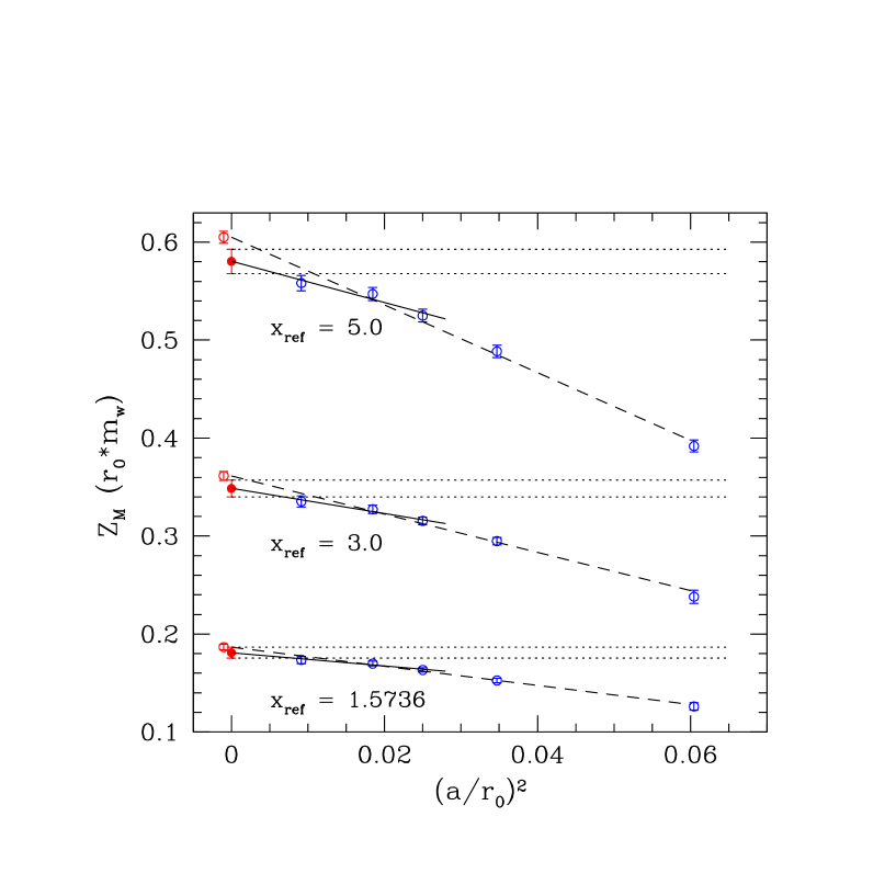
Figure 1: Cutoff effects in $Z_{\rm M}^{\rm w}\,(r_{0}\,m_{\rm w})$ for $x_{\rm{ref}}=1.5736$, $3.0$ and $5.0$. The continuum estimates for $U_{\rm M}$ of eq. (3.14) are represented by the error band (dotted lines). The corresponding linear fits in $(a/r_{0})^{2}$ to data computed for $\beta\geq 6.1$ are shown as the solid lines. Extrapolations using data at all five values of the lattice spacings are represented by the dashed lines.

Before undertaking this calculation, we wish to discuss the issue of discretization errors in our renormalization condition, eq. (2.8). To this end we note that a valid definition of $Z_{\rm M}$ is also provided by the right-hand side of eq. (2.6) evaluated at non-zero $g_{0}^{\prime}$. The two expressions differ by O($a^{2}$) discretization errors associated with the intermediate Wilson regularization. In eq. (2.6) these errors are present, while they are not in eq. (2.8), owing to the continuum extrapolation in the definition of $U_{\rm M}$. One might think that such O($a^{2}$) artefacts – which are formally of the same or even higher order than those of most other lattice regularizations – are unimportant. We are now going to show that this is not the case. To this end we have evaluated

$$Z_{\rm M}^{\rm w}(g_{0}^{\prime})\times(r_{0}m_{\rm w})(g_{0}^{\prime})\Big{|}_{(r_{0}\,m_{\rm P})^{2}=x_{\rm ref},}\quad x_{\rm ref}=1.5736,\,3.0,\,5.0$$ (3.15)

for bare couplings $g_{0}^{\prime}$ corresponding to $\beta=5.85,6.0,6.1,6.2$ and 6.45. Data for $\beta\geq 6.0$ were taken from ref. [?]. The results for $(r_{0}m_{\rm w})$ at $\beta=5.85$ were obtained as described in Section 4 below. The value for $Z_{\rm M}^{\rm w}$ at $\beta=5.85$ was estimated by extrapolating the parameterization of eq. (6.10) in [?] and doubling the error.

The approach to the continuum limit is shown in Fig. 1. The first observation is that lattice artefacts in $Z_{\rm M}^{\rm w}\,(r_{0}m_{\rm w})$ appear to be consistent with the expected $a^{2}$ behaviour – at least for $x_{\rm ref}=1.5736$ and 3.0: performing linear fits in $(a/r_{0})^{2}$ to data points at all five values of the lattice spacing produce good $\chi^{2}/{\rm{dof}}$. Furthermore, as can be seen from the figure, the results in the continuum limit are compatible with the estimates for $U_{\rm M}$ in eq. (3.14). The latter were obtained by excluding all points below $\beta=6.1$ from the continuum extrapolations, as a safeguard against potentially large cutoff effects of higher order. As can be seen from the figure, such discretization effects appear to be larger at $x_{\rm ref}=5.0$, which certainly justifies the exclusion of those data points obtained on the two coarser lattices.

The deviation of $Z_{\rm M}^{\rm{w}}(r_{0}m_{\rm w})$ from its continuum value amounts to about 20% at $\beta=6.0$ and 40% at $\beta=5.85$. Thus, if $Z_{\rm M}$ were evaluated using eq. (2.6) with $g_{0}^{\prime}=g_{0}$ instead of eq. (2.8), the result at $\beta=5.85$ would be 40% smaller, due entirely to cutoff effects of order $a^{2}$ in the intermediate Wilson regularization.

This discussion underlines that it is important to use the continuum result $U_{\rm M}$ in the renormalization condition. It guarantees that the approach to the continuum limit of quantities for which these renormalization constants are used is not obscured by lattice artefacts of O($a^{2}$), introduced by using O($a$)-improved Wilson fermions as an intermediate regularization.

As can be inferred from eq. (3.14), the factor $U_{\rm M}$ is known with a precision of about 3%. At present this presents a lower bound on the accuracy in the determination of renormalization factors according to our proposal. One might argue that more precise estimates for $U_{\rm{M}}$ could be obtained by including the data with $\beta\leq 6.0$ in the continuum extrapolation. We have still decided against this, in order to be certain about excluding effects from higher orders in the lattice spacing. Also, given the high cost of simulations employing discretizations such as overlap fermions, it will be some time before the lower bound of 3% will be regarded as a real limitation. If one wants to improve the accuracy in the determination of $U_{\rm M}$, it would be preferable to add data points at smaller lattice spacings, which should be possible with a relatively modest amount of computer time.

4 Lattice calculation of pseudoscalar masses

We now describe the details of our calculation of pseudoscalar two-point functions using the overlap operator as well as O($a$)-improved Wilson fermions at $\beta=5.85$. Although our strategy only requires published results for Wilson fermions, the additional Wilson calculations performed for different lattice sizes provide us with valuable information about finite-size effects at a much lower cost than with overlap fermions.

4.1 Simulation details

For the massive overlap operator $D_{N}$ we use the following definition

$$D_{N}=\left(1-\frac{am_{\rm ov}}{2(1+s)}\right)D_{N}^{(0)}+m_{\rm ov},$$ (4.16)

where

$$aD_{N}^{(0)}=(1+s)\left(1-A/\sqrt{A^{\dagger}A}\right),\quad A\equiv 1+s-aD_{W},$$ (4.17)

and $D_{W}$ is the standard Wilson-Dirac operator. The naive continuum limit of $D_{N}$ is the canonically normalized Dirac operator with a bare quark mass $m_{\rm ov}$. The parameter $s$ was fixed at $s=0.6$, which is close to the value where the localization of the operator was found to be optimal at this $\beta$ value [?]. The numerical implementation of the inverse square root in eq. (4.16) was performed using a Chebyshev approximation, and for further details we refer to our earlier work [?]. Here we only mention that we have employed a multi-mass solver [?], which allows for a simultaneous calculation of the quark propagators for seven values of the bare mass ranging from $am_{\rm ov}=0.047-0.188$.

In order to compute pseudoscalar meson masses and current quark masses for O($a$)-improved Wilson fermions we have followed the same procedure as in ref. [?]. In particular, we have employed Schrödinger functional boundary conditions on lattice sizes $L/a=8,10,12$ and 16, with $T/a=24$ fixed, in order to study finite-size effects. For the improvement coefficients $c_{\rm sw}$ and $c_{\rm A}$, which appear in the definition of the improved action and axial current, respectively, we have chosen

$$c_{\rm sw}=1.909,\qquad c_{\rm A}=-0.144.$$ (4.18)

The value for $c_{\rm sw}$ was obtained from the interpolating formula eq. (4) of ref. [?]. To our knowledge a non-perturbative result for the coefficient $c_{\rm A}$ has so far not been published for $\beta<6.0$. The choice in eq. (4.18) is based on a non-perturbative calculation using the SF, which is described in detail in Appendix A.

While it can be shown that there are no exceptional configurations for the overlap operator at non-zero quark mass [?,?,?], this is not the case for Wilson fermions. Indeed, when working below $\beta=6.0$ the incidence of exceptional configurations may be so high – especially for quark masses below that of the strange quark – so as to make a reliable calculation of quark and meson masses impossible.

For our calculations of quark propagators using Wilson fermions we have chosen relatively heavy quarks, with unrenormalized current quark masses in the range $80-120\,{\rm MeV}$. Only on the smaller volumes of $L/a=8,\,10$ did we push to lighter quarks, corresponding to 65 MeV. We checked against the occurrence of exceptional configurations by plotting the Monte Carlo history of the correlation functions of the axial current and pseudoscalar density evaluated at $x_{0}=T/2$. Exceptional configurations manifest themselves as isolated peaks (or dips) whose heights exceed the typical statistical fluctuations by several orders of magnitude. Although one candidate each was detected for $L/a=8$ and 10, the observed fluctuations were not deemed large enough to justify the exclusion of these configurations from the statistical ensembles. Hence, for the case of Wilson fermions, all hadron and quark masses have been evaluated using the full statistics on all lattices.

4.2 Results for pseudoscalar masses

$L/a$	configs.	$\kappa$	$am_{\rm w}$	$am_{\rm P}$	$(am_{\rm P})^{2}$
8	640	0.13150	0.07309(37)	0.5780(45)	0.3342(52)
		0.13200	0.06106(40)	0.5265(49)	0.2772(51)
		0.13250	0.04893(47)	0.4707(54)	0.2216(50)
		0.13300	0.03685(52)	0.4085(60)	0.1668(49)
10	512	0.13150	0.07362(27)	0.6002(29)	0.3602(35)
		0.13200	0.06174(28)	0.5496(31)	0.3021(35)
		0.13250	0.04991(30)	0.4948(35)	0.2449(35)
		0.13300	0.03805(34)	0.4338(40)	0.1882(35)
12	256	0.13150	0.07436(30)	0.6005(30)	0.3606(36)
		0.13200	0.06249(32)	0.5503(33)	0.3028(36)
		0.13250	0.05067(35)	0.4961(36)	0.2461(36)
16	150	0.13150	0.07458(24)	0.6065(21)	0.3678(26)
		0.13200	0.06277(25)	0.5573(23)	0.3106(26)
		0.13250	0.05102(27)	0.5045(26)	0.2545(26)

Table 1: Lattice sizes, statistics, pseudoscalar and current quark masses computed using O(a)-improved Wilson fermions.

$am_{\rm ov}$	$am_{\rm P}$	$(am_{\rm P})^{2}$
0.047	0.311(31)	0.096(20)
0.063	0.357(22)	0.128(16)
0.078	0.398(17)	0.159(14)
0.097	0.444(14)	0.197(13)
0.125	0.506(12)	0.256(13)
0.161	0.579(11)	0.335(12)
0.188	0.630(10)	0.397(12)

Table 2: Pseudoscalar masses extracted from single-mass fits in the interval $6\leq x_{0}/a\leq 12$ at several values of the bare mass $m_{\rm ov}$.

The results for the pseudoscalar and bare current quark masses computed for O($a$)-improved Wilson fermions are presented in Table 1. The masses were extracted following the procedure described in detail in ref. [?]. In particular, the estimates for the pseudoscalar masses listed in the table were obtained by averaging the effective masses computed from the correlation function of the improved axial current. In accordance with Table 1 of [?], and using $r_{0}/a=4.067\pm 0.014$ [?] we have chosen the time window $11\leq x_{0}/a\leq 15$ for the averaging procedure. Estimates for the bare current quark mass were obtained in a similar manner, by averaging the results over the interval $10\leq x_{0}/a\leq 16$. This choice of time window coincides with a clear plateau observed for this quantity.

By comparing the results in Table 1 obtained on different lattice sizes, one observes that the time interval $11\leq x_{0}/a\leq 15$ suggested in [?] produces consistent results for pseudoscalar masses if $L/a\geq 10$. By contrast, using a spatial lattice size of $L/a=8$ (corresponding to $L\approx 1\,{\rm fm}$) leads to finite-size effects at the level of 4% (4 standard deviations). Choosing a shorter time window on $L/a=8$, such as $11\leq x_{0}/a\leq 13$, brings the results closer to those on the larger volumes, but a 2% effect (1.5 standard deviations) remains.

On the other hand, for $L/a\geq 10$ (i.e. $L\geq 1.2\,{\rm fm}$) finite-size effects in the pseudoscalar mass are of the order of 1.5% or less. In order to exclude large finite-size effects for pseudoscalar masses computed using the overlap operator, whilst keeping the computational overheads small, we have thus decided to work with $L/a=10$. However, the above analysis of finite-size effects only applies to pseudoscalar meson masses with $am_{\rm P}\;\raisebox{-2.58334pt}{$\stackrel{{\scriptstyle\textstyle{>}}}{{\sim}}$}\;0.5$, a range which lies above the reference points $x_{\rm ref}=1.5736$ and 3.0. This was our main reason to consider the reference point $x_{\rm ref}=5.0$ in addition: at $\beta=5.85$ this choice corresponds to $am_{\rm P}\approx 0.55$, a value for which the absence of significant finite-volume effects has been confirmed.

In Table 2, we present the results for pseudoscalar masses computed using the overlap operator on an ensemble of 50 configurations. The chosen lattice size was $L/a=10,\,T/a=24$, with periodic boundary conditions in all space-time directions. After averaging the correlation functions over the forward and backward directions in euclidean time, we extracted the masses from single-cosh fits to the correlation functions in the interval $6\leq x_{0}/a\leq 12$. The quoted statistical errors were obtained from a jackknife procedure. We have classified configurations according to their topological index, distinguishing between topological (having a non-zero index) and non-topological configurations and determined the average pseudoscalar masses restricted to either class. Only very near the chiral limit does one expect these quantities to differ. In the range of quark masses considered we did not detect any difference between the two classes, so that we could safely include all topologies in the average.

In Fig. 2, we show the results for the behaviour of $(am_{\rm P})^{2}$ as a function of $am_{\rm ov}$ and $am_{\rm w}$. In both cases the results are perfectly compatible with the linear behaviour expected in lowest order Chiral Perturbation Theory. As an illustration we have plotted the results from a chiral fit to our data, using the linear parameterization

$$(am_{\rm P})^{2}=A_{i}+B_{i}\cdot(am_{i}),\quad i=\hbox{ov,\,w},$$ (4.19)

thus allowing for a non-zero intercept of $(am_{\rm P})^{2}$ at vanishing quark mass. The results of these fits are:

$$A_{\rm ov}=-0.009(18), B_{\rm ov}=2.139(80),$$ (4.20)

$$A_{\rm w}=\phantom{-}0.0039(39), B_{\rm w}=4.836(44),$$ (4.21)

where we have used all seven data points in the overlap case and all four quark masses in the Wilson set. Note that in both cases the intercepts are perfectly compatible with zero within errors.

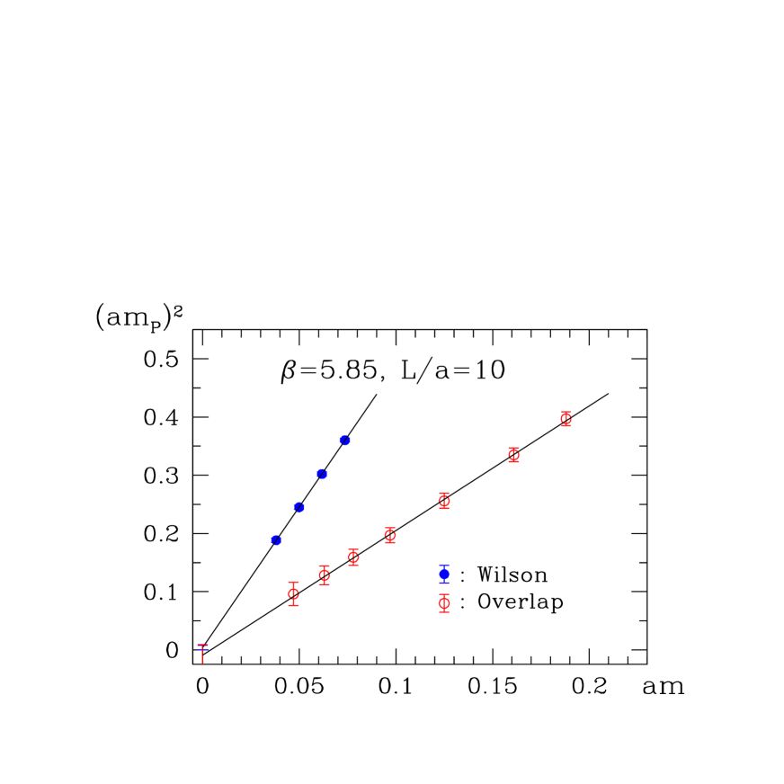
Figure 2: $m_{\rm P}^{2}$ versus $m_{\rm ov}$ (open circles) and $m_{\rm w}$ (filled circles) respectively for overlap and $O(a)$-improved Wilson fermions. The solid lines are the fits of eqs. (4.20) and (4.21).

Pseudoscalar propagators for overlap fermions have been studied before in [?] for $\beta=5.7,5.85$ and 6.0, thus enabling a direct comparison with our results.. Since the authors of [?] do not present numbers for $(am_{\rm P})^{2}$ one has to infer its quark mass behaviour by reading the data off their plots. From this fairly crude comparison we conclude that the slope parameter $B_{\rm ov}$ is in rough agreement with our findings. Unlike the authors of [?] we did not attempt to model the quark mass behaviour including quenched chiral logarithms. Judging from the quality of our fits to eq. (4.19) we do not expect a significant deviation from leading order Chiral Perturbation Theory at our level of statistics in the range of quark masses we consider. In order to test for the presence of quenched chiral logarithms, it may be necessary to go to much smaller masses than our lightest quark, whose mass is roughly half as large as that of the strange quark.

5 Results and discussion

5.1 Non-perturbative result for $\widehat{Z}_{\rm S}$

We have now the necessary results to compute the renormalization factor $\widehat{Z}_{\rm S}$ for the RGI condensate using eqs. (2.8) and (2.13). Our task is to determine $(r_{0}m_{\rm ov})$ at the reference value $x_{\rm ref}$, which could in principle be achieved using the results of the chiral fit, eq. (4.20). However, we prefer to perform local interpolations of the quark mass $m_{\rm ov}$ to the reference point, which avoids any assumption about the mass behaviour of $(am_{\rm P})^{2}$ at or very near the chiral limit.

To this end we have interpolated $(r_{0}m_{\rm ov})$ to our chosen values of $x_{\rm{ref}}$ by using the three nearest data points for $(r_{0}\,m_{\rm P})^{2}$. We obtain

$$(r_{0}\,m_{\rm ov})\Big{|}_{(r_{0}m_{\rm P})^{2}=x_{\rm ref}}=\left\{\begin{array}[]{cl}0.190(44),&\quad x_{\rm ref}=1.5736\\ 0.363(26),&\quad x_{\rm ref}=3.0\\ 0.594(23),&\quad x_{\rm ref}=5.0.\end{array}\right.$$ (5.22)

We add that these results are entirely consistent with interpolations using only the two neighbouring points. Given the almost perfect linearity of the quark mass dependence of $(r_{0}m_{\rm P})^{2}$, it is not surprising that interpolations using all seven data points are also consistent. Hence we regard the uncertainties in our results of eq. (5.22) as conservative estimates.

By combining the results for $(r_{0}\,m_{\rm ov})$ with the factor $U_{\rm M}$ we obtain

$$\widehat{Z}_{\rm S}=\left\{\begin{array}[]{ll}1.05(25),&\quad x_{\rm ref}=1.5736\\ 1.04(8),&\quad x_{\rm ref}=3.0\\ 1.02(4),&\quad x_{\rm ref}=5.0,\end{array}\right.\quad\beta=5.85.$$ (5.23)

The results at the three values of $x_{\rm ref}$ are consistent within even the smallest of the statistical errors. This indicates that our renormalization condition may be applied over a fairly large range of quark masses without introducing significant discretization errors due to working at non-zero quark mass. It also indicates that finite-volume effects, even at the lightest reference point, appear to be small. Owing to the modest statistics in our simulations, the errors in $\widehat{Z}_{\rm S}$ in eq. (5.23) are clearly dominated by the limited accuracy of the estimates for $(r_{0}\,m_{\rm ov})$ at the reference points, which amounts to 24%, 8% and 4% at $x_{\rm ref}=1.5736$, 3.0 and 5.0, respectively. This is larger than the relative error in $U_{\rm M}$ of about 3%. However, with better statistics, it should be easy to obtain more accurate estimates for $(r_{0}\,m_{\rm ov})$ and thus $\widehat{Z}_{\rm S}$.

The dependence on the value of $x_{\rm ref}$ is quite weak and well covered by the statistical uncertainty. We quote the result for $x_{\rm ref}=3.0$ as our best estimate, since this reference point is a good compromise between being chiral enough so as not to introduce significant discretization errors, and massive enough to guarantee negligible finite-size effects. Thus we obtain

$$\begin{array}[]{rl}\widehat{Z}_{\rm S}&=1.04\pm 0.08\\ Z_{\rm S}(2\,{\rm GeV})&=1.44\pm 0.11,\end{array}\quad\beta=5.85,$$ (5.24)

These numbers are the main result of this paper. All systematics associated with the intermediate Wilson regularization have been eliminated by the continuum extrapolation in the definition of the universal factor $U_{\rm M}$. As discussed in Section 4, we have verified that finite-volume effects are under control. Discretization errors of order $(am)^{2}$ in our determination of $\widehat{Z}_{\rm S}$ seem to be small, as indicated by the consistency of our results at the three reference values.

5.2 Comparison with perturbation theory

In ref. [?] the perturbative renormalization of quark bilinears was studied for the overlap operator. The one-loop expression for $Z_{\rm S}$ reads

$$Z_{\rm S}^{\rm pt}(g_{0},\mu)=1+g_{0}^{2}\left[\frac{1}{2\pi^{2}}\ln(a\mu)+z_{\rm S}^{(1)}\right]+O(g_{0}^{4}),$$ (5.25)

where the one-loop coefficient $z_{\rm S}^{(1)}$ depends on the parameter $s$ in the definition of the overlap operator. For our value of $s=0.6$ one finds [?]

$$z_{\rm S}^{(1)}=0.107074.$$ (5.26)

It is well known that perturbation theory in the bare coupling $g_{0}$ is not very convergent. As a consequence it has become customary to consider “mean-field improved” estimates for perturbative renormalization factors [?,?]. Another proposal is based on the resummation of “cactus” diagrams [?]. Here, in the spirit of [?], we propose the following mean-field improved expression:

$$Z_{\rm S}^{\rm mf}(g_{0},\mu)=\left(\frac{1+s}{1+\tilde{s}}\right)\left\{1+g^{2}\left[\frac{1}{2\pi^{2}}\ln(a\mu)+z_{\rm S}^{(1)}+u_{0}^{(1)}\left(\frac{3-s}{1+s}\right)\right]\right\}\ ,$$ (5.27)

where $\tilde{s}=3+(s-3)/u_{0}$. We take $u_{0}^{4}$ to be the average plaquette in infinite volume, and $u_{0}^{(1)}=-1/12$ is the one-loop coefficient in its perturbative expansion. At this order, the choice of coupling, $g$, is ambiguous. For consistency, we work with the coupling used in obtaining the renormalization group factor in eq. (2.12), i.e. $g^{2}=2.5432$. We can now evaluate eq. (5.27) using lattice data for the average plaquette and by setting the lattice spacing at $\beta=5.85$ with the help of the interpolating formula for the hadronic radius $r_{0}/a$ [?]. For $u_{0}^{4}=0.575$ the results for $\widehat{Z}_{\rm S}^{\rm mf}$ and $Z_{\rm S}^{\rm mf}$ are

$$\begin{array}[]{rl}Z_{\rm S}^{\rm mf}(2\,{\rm GeV})&=1.26\\ \widehat{Z}_{\rm S}^{\rm mf}&=0.91,\end{array}\quad\beta=5.85.$$ (5.28)

Comparing these mean-field improved perturbative estimates to the non-perturbative results of eq. (5.24), one finds that the former are about 12% smaller. This is a significant improvement on the results of bare perturbation theory, where $Z_{\rm S}^{\rm pt}(2\,{\rm GeV})=1.12$ as given by eq. (5.25), which are more than 20% smaller than the non-perturbative results of eq. (5.24).

6 Summary and conclusions

We have proposed and tested a method to non-perturbatively renormalize scalar and pseudoscalar densities for fermionic discretizations which preserve chiral symmetry at non-zero lattice spacing. This method also provides a means to renormalize quark masses non-perturbatively in any lattice regularization. Given the cost of simulations employing Ginsparg-Wilson fermions and the incompatibility of Schrödinger functional boundary conditions with the Ginsparg-Wilson equation, we found it advantageous to proceed through O($a$)-improved Wilson fermions, where the non-perturbative renormalization of currents and densities has already been studied extensively. The sought-after renormalization constants are then obtained through a matching of RGI quark masses at fixed pseudoscalar meson mass. As evident in eq. (2.8), all reference to Wilson fermions drops out, owing to the universal factor $U_{\rm M}$ defined and evaluated in the continuum limit. Furthermore, the overhead for implementing the matching condition should be negligible in most cases, since it relies on quantities that are commonly computed in phenomenological studies where the renormalization constants are likely to be used. The idea to use an intermediate lattice regularization which is relatively cheap to implement may prove useful for the computation of other renormalization constants in fermionic discretizations that are numerically much more demanding.

As an application, we have computed the renormalization constants which are required for the quark condensate obtained using overlap fermions in the quenched approximation. Our results at $\beta=5.85$ are listed in eq. (5.24) and can now be combined with the result for the subtracted bare condensate determined in [?], i.e. $a^{3}\Sigma_{\rm sub}=0.00323(37)$ . In units of $r_{0}$ we obtain

$$\begin{array}[]{rl}r_{0}^{3}\widehat{\Sigma}&=0.226(26)(2)(17)\\ r_{0}^{3}\Sigma_{\rm\overline{MS\kern-0.35002pt}\kern 0.35002pt}(2\,{\rm GeV})&=0.313(36)(3)(23),\end{array}\quad\beta=5.85,$$ (6.29)

where the first error is due to the statistical uncertainty in $a^{3}\Sigma_{\rm sub}$, the second corresponds to the error in $r_{0}/a$, and the third arises from the error in the renormalization factors $\widehat{Z}_{\rm S}$ and $Z_{\rm S}$, respectively. Combining all but the error associated with $r_{0}/a$ in quadrature and using $r_{0}=0.5\,{\rm fm}$ we find

$$\begin{array}[]{rl}\widehat{\Sigma}&=\left(240\pm 11\,{\rm MeV}\right)^{3}\times\left(\displaystyle\frac{a^{-1}[{\rm MeV}]}{1605\,{\rm MeV}}\right)^{3}\\ \Sigma_{\rm\overline{MS\kern-0.35002pt}\kern 0.35002pt}(2\,{\rm GeV})&=\left(268\pm 12\,{\rm MeV}\right)^{3}\times\left(\displaystyle\frac{a^{-1}[{\rm MeV}]}{1605\,{\rm MeV}}\right)^{3}\end{array}\quad\beta=5.85.$$ (6.30)

These results are still subject to discretization errors of O($a^{2}$). A detailed discussion of lattice artefacts and other systematic errors – including the scale ambiguity in the quenched approximation – as well as a comparison of these results with those obtained through other approaches is deferred to our companion paper [?].

Acknowledgements.

We are grateful to Martin Lüscher, Stefan Sint and Rainer Sommer for useful and stimulating discussions. We thank the computer centres at NIC (Jülich) and DESY Zeuthen for providing computer time and technical support.

Appendix A Determination of $c_{\rm A}$ at $\beta=5.85$

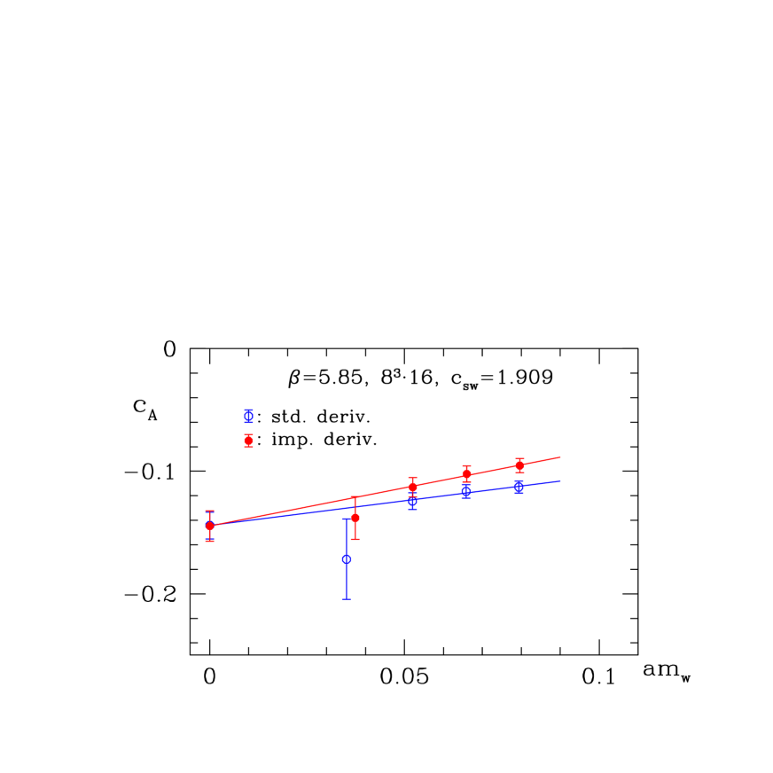
Figure 3: The chiral extrapolation of $c_{\rm A}$ using the three heaviest quark masses. Data for the standard and improved definitions of the lattice derivative are denoted by the open and filled symbols, respectively.

Figure 4: The result for $c_{\rm A}$ at $\beta=5.85$ (filled circle) compared with the results from ref. [?] (open circles). The solid curve is the interpolating formula valid for $6.0\leq\beta$. The dashed curve denotes perturbation theory in the bare coupling, whereas the crosses represent the estimates in mean-field improved perturbation theory.

While a non-perturbative value for the improvement coefficient $c_{\rm sw}$ is available at $\beta=5.85$ [?], the coefficient $c_{\rm A}$ of the improved axial current, which is required for the current quark mass, is not known for $\beta<6.0$.

As mentioned in Sect. 4, numerical simulations using Wilson fermions are hampered by the occurrence of exceptional configurations associated with unphysical zero modes of the Wilson-Dirac operator. This problem is further exacerbated by working at $a\;\raisebox{-2.58334pt}{$\stackrel{{\scriptstyle\textstyle{>}}}{{\sim}}$}\;0.1\,{\rm fm}$ (i.e. $\beta\;\raisebox{-2.58334pt}{$\stackrel{{\scriptstyle\textstyle{<}}}{{\sim}}$}\;6.0$) and small quark masses. However, if one is willing to relax the requirement that the improvement conditions for $c_{\rm sw}$ and $c_{\rm A}$ be evaluated at or very near the chiral limit [?], the occurrence of exceptional configurations may be sufficiently suppressed. Thus, an extension of the determination of improvement coefficients to the regime where $\beta<6.0$ may be possible.

In order to determine $c_{\rm A}$ at $\beta=5.85$ we have chosen $c_{\rm sw}=1.909$ [?] and followed the strategy of ref. [?]. It has been observed [?], though, that the original improvement condition for $c_{\rm A}$ used in [?] suffers from a loss of numerical accuracy towards larger values of the bare coupling, corresponding to $\beta\approx 6.0$. A modified, but closely related improvement condition for $c_{\rm A}$ has been proposed and tested [?]. It was shown that the alternative condition’s numerical sensitivity does not deteriorate at large couplings. Furthermore, it gives consistent results compared with the original condition, thereby confirming the determination of $c_{\rm A}$ in ref. [?].

We have evaluated both the original and modified improvement condition at $\beta=5.85$ on a $8^{3}\cdot 16$ lattice. We used the same four values of the hopping parameter listed in Table 1. With the procedure outlined in Sect. 4 to check against the occurrence of exceptional configurations, we eliminated two configurations from the original ensemble of 2560. It was found that the alternative improvement condition gave a stable signal for $c_{\rm A}$ at the three heaviest quark masses. By contrast, the original improvement condition used in [?] performed so badly at $\beta=5.85$ that it could not be used to determine $c_{\rm A}$.

Our estimates for $c_{\rm A}$ obtained at non-zero quark masses shows some dependence on the quark mass, and therefore our final result is obtained through a chiral extrapolation as shown in Fig. 3. We have also evaluated the improvement condition using a higher-order lattice derivative [?], which was found to have a significant impact on the determination of some improvement coefficients [?]. The corresponding results and extrapolation are also shown in Fig. 3. Both definitions of the lattice derivative give entirely consistent results in the chiral limit, and as our final result we quote

$$c_{\rm A}=-0.144\pm 0.011,\qquad\beta=5.85.$$ (A.31)

This value is shown together with the previous determination of $c_{\rm A}$ for $\beta\geq 6.0$ [?] in Fig. 4.

Finally we note that we have also estimated $c_{\rm A}$ using the method proposed in ref. [?] (see also [?,?]). We have confirmed the observation of [?], namely that the accuracy of the method is limited by the relatively small range in $x_{0}$ in which a stable signal is obtained. On our $8^{3}\cdot 16$ lattice the method of [?] produces results which are entirely consistent with the estimate in eq. (A.31).

References

- [1] R. Gupta and T. Bhattacharya, Phys. Rev. D55 (1997) 7203, hep-lat/9605039.
- [2] L. Giusti, F. Rapuano, M. Talevi and A. Vladikas, Nucl. Phys. B538 (1999) 249, hep-lat/9807014.
- [3] R.G. Edwards, U.M. Heller and R. Narayanan, Phys. Rev. D59 (1999) 094510, hep-lat/9811030.
- [4] P.H. Damgaard, R.G. Edwards, U.M. Heller and R. Narayanan, Phys. Rev. D61 (2000) 094503, hep-lat/9907016.
- [5] P. Hernández, K. Jansen and L. Lellouch, Phys. Lett. B469 (1999) 198, hep-lat/9907022.
- [6] MILC Collaboration (T. DeGrand), Phys. Rev. D63 (2001) 034503, hep-lat/0007046.
- [7] T. Blum et al., (2000), hep-lat/0007038.
- [8] P.H. Ginsparg and K.G. Wilson, Phys. Rev. D25 (1982) 2649.
- [9] F. Niedermayer, Nucl. Phys. Proc. Suppl. 73 (1999) 105, hep-lat/9810026.
- [10] M. Lüscher, Nucl. Phys. Proc. Suppl. 83 (2000) 34, hep-lat/9909150.
- [11] H. Neuberger, Nucl. Phys. Proc. Suppl. 83 (2000) 67, hep-lat/9909042.
- [12] A. Hasenfratz et al., Nucl. Phys. B356 (1991) 332.
- [13] H. Neuberger, Phys. Lett. B417 (1998) 141, hep-lat/9707022.
- [14] S. Sint, Nucl. Phys. Proc. Suppl. 94 (2001) 79, hep-lat/0011081.
- [15] G. Martinelli, C. Pittori, C.T. Sachrajda, M. Testa and A. Vladikas, Nucl. Phys. B445 (1995) 81, hep-lat/9411010.
- [16] K. Jansen et al., Phys. Lett. B372 (1996) 275, hep-lat/9512009.
- [17] V. Giménez, L. Giusti, F. Rapuano and M. Talevi, Nucl. Phys. B540 (1999) 472, hep-lat/9801028.
- [18] D. Becirevic et al., Phys. Lett. B444 (1998) 401, hep-lat/9807046.
- [19] ALPHA & UKQCD Collaborations (J. Garden, J. Heitger, R. Sommer and H. Wittig), Nucl. Phys. B571 (2000) 237, hep-lat/9906013.
- [20] JLQCD Collaboration (S. Aoki et al.), Phys. Rev. Lett. 82 (1999) 4392, hep-lat/9901019.
- [21] T. Blum et al., (2001), hep-lat/0102005.
- [22] P. Hernández, K. Jansen, L. Lellouch and H. Wittig, in preparation.
- [23] C. Alexandrou, E. Follana, H. Panagopoulos and E. Vicari, Nucl. Phys. B580 (2000) 394, hep-lat/0002010.
- [24] ALPHA Collaboration (S. Capitani, M. Lüscher, R. Sommer and H. Wittig), Nucl. Phys. B544 (1999) 669, hep-lat/9810063.
- [25] R. Sommer, Nucl. Phys. B411 (1994) 839, hep-lat/9310022.
- [26] P. Hernández, K. Jansen and M. Lüscher, Nucl. Phys. B552 (1999) 363, hep-lat/9908010.
- [27] B. Jegerlehner, Nucl. Phys. Proc. Suppl. 63A-C (1998) 958, hep-lat/9708029.
- [28] ALPHA Collaboration (M. Guagnelli, J. Heitger, R. Sommer and H. Wittig), Nucl. Phys. B560 (1999) 465, hep-lat/9903040.
- [29] R.G. Edwards, U.M. Heller and T.R. Klassen, Phys. Rev. Lett. 80 (1998) 3448, hep-lat/9711052.
- [30] P. Hasenfratz, V. Laliena and F. Niedermayer, Phys. Lett. B427 (1998) 125, hep-lat/9801021.
- [31] M. Lüscher, Phys. Lett. B428 (1998) 342, hep-lat/9802011.
- [32] ALPHA Collaboration (M. Guagnelli, R. Sommer and H. Wittig), Nucl. Phys. B535 (1998) 389, hep-lat/9806005.
- [33] S. Dong, F. Lee, K. Liu and J. Zhang, Phys. Rev. Lett. 85 (2000) 5051, hep-lat/0006004.
- [34] G. Parisi, (1980), Presented at 20th Int. Conf. on High Energy Physics, Madison, Wis., Jul 17-23, 1980.
- [35] G.P. Lepage and P.B. Mackenzie, Phys. Rev. D48 (1993) 2250, hep-lat/9209022.
- [36] M. Lüscher, S. Sint, R. Sommer, P. Weisz and U. Wolff, Nucl. Phys. B491 (1997) 323, hep-lat/9609035.
- [37] M. Guagnelli and R. Sommer, private notes (unpublished) (1998).
- [38] G.M. de Divitiis and R. Petronzio, Phys. Lett. B419 (1998) 311, hep-lat/9710071.
- [39] ALPHA Collaboration (M. Guagnelli et al.), Nucl. Phys. B595 (2001) 44, hep-lat/0009021.
- [40] T. Bhattacharya, S. Chandrasekharan, R. Gupta, W. Lee and S. Sharpe, Phys. Lett. B461 (1999) 79, hep-lat/9904011.
- [41] T. Bhattacharya, R. Gupta, W. Lee and S. Sharpe, Phys. Rev. D63 (2001) 074505, hep-lat/0009038.
- [42] UKQCD Collaboration (S. Collins and C.T.H. Davies), Nucl. Phys. Proc. Suppl. 94 (2001) 608, hep-lat/0010045.