UTCCP-P-107 Topological Susceptibility in Lattice QCD with Two Flavors of Dynamical Quarks

Abstract

We present a study of the topological susceptibility in lattice QCD with two degenerate flavors of dynamical quarks. The topological charge is measured on gauge configurations generated with a renormalization group improved gauge action and a mean field improved clover quark action at three values of $\beta=6/g^{2}$, corresponding to lattice spacings of $a\approx 0.22$, 0.16 and 0.11 fm, with four sea quark masses at each $\beta$. The study is supplemented by simulations of pure SU(3) gauge theory with the same gauge action at 5 values of $\beta$ with lattice spacings 0.09 fm$\,\hbox to0.0pt{\lower 3.5pt\hbox{$\mathchar 0\relax\sim$}\hss}\raise 1.0pt\hbox{$<$}\,a\,\hbox to0.0pt{\lower 3.5pt\hbox{$\mathchar 0\relax\sim$}\hss}\raise 1.0pt\hbox{$<$}\,$0.27 fm. We employ a field theoretic definition of the topological charge together with cooling. For the topological susceptibility in the continuum limit of pure SU(3) gauge theory we obtain $\chi_{t}^{1/4}=197^{+13}_{-16}$ MeV where the error shows statistical and systematic ones added in quadrature. In full QCD $\chi_{t}$ at heavy sea quark masses is consistent with that of pure SU(3) gauge theory. A decrease of $\chi_{t}$ toward light quark masses, as predicted by the anomalous Ward-Takahashi identity for U(1) chiral symmetry, becomes clearer for smaller lattice spacings. The cross-over in the behavior of $\chi_{t}$ from heavy to light sea quark masses is discussed.

I Introduction

The topological structure of gauge field fluctuations, in particular instantons, has been invoked to explain several important low energy properties of QCD including the breaking of axial U(1) symmetry and the large mass of the $\eta^{\prime}$ meson. Numerical simulations on a space-time lattice provide a non-perturbative tool for the study of these phenomena beyond semiclassical approximations.

Lattice studies of the topological susceptibility $\chi_{t}$ as a measure of these fluctuations have been mostly carried out for pure gauge theory without the presence of dynamical fermions [1]. Recent determinations by various groups using different methods have led to a consistent value in SU(3) gauge theory of $\chi_{t}^{1/4}=200\pm 18$ MeV [1].

Sea quark effects on the topological susceptibility have been much less studied, although dynamical quarks are expected to have a strong influence on $\chi_{t}$ leading to a complete suppression for massless quarks. From the anomalous Ward-Takahashi identity for U(1) chiral symmetry, the topological susceptibility is predicted [2, 3, 4] to obey for small quark masses in the chirally broken phase,

$$\chi_{t}=\frac{\Sigma}{N_{f}}m_{q}+O(m_{q}^{2}),\;\;\Sigma=-\lim_{m_{q}\rightarrow 0}\lim_{V\rightarrow\infty}\langle\overline{\psi}\psi\rangle.$$ (1)

It is an interesting question to investigate whether lattice data confirm a suppression consistent with Eq. (1).

Pioneering attempts to calculate $\chi_{t}$ in full QCD [5, 6, 7] were restricted to small statistics and were plagued by long autocorrelation times. Progress in the simulation of full QCD, as well as increase of available computer power in recent years, has enabled this question to be readdressed with a higher accuracy. A number of pieces of work have been reported recently [8, 9, 10, 11, 12, 13] coming to different conclusions whether the topological susceptibility is consistent with the prediction of Eq. (1). A common shortcoming in Refs. [8, 9, 10, 11, 12] is that they have been made at only one lattice spacing. Ref. [13], on the other hand, used only one bare quark mass $am_{q}$ at each coupling constant $\beta$.

In this article we attempt to improve on this status by calculating the topological susceptibility in full QCD with two flavors of dynamical quarks at four sea quark masses at each of three gauge couplings. We perform calculations on configurations of the CP-PACS full QCD project [14]. These have been generated on the CP-PACS parallel computer [15] using a renormalization group (RG) improved gauge action [16] and a mean field improved Sheikholeslami-Wohlert clover quark action [17]. The efficacy of this choice of action over the standard action has been demonstrated in Ref. [18] by examining both the rotational symmetry of the static quark potential and the scaling behavior of light hadron mass ratios.

Preliminary results for the topological susceptibility based on a first analysis at our intermediate lattice spacing have been published in Ref. [8]. In this article we present the final analysis and results at all gauge couplings.

The identification of dynamical quark effects requires a comparison with pure SU(3) gauge theory where sea quarks are absent. We therefore supplement our study of topology in full QCD by a set of simulations of SU(3) gauge theory with the same RG-improved gluon action at a similar range of lattice spacings.

The outline of this article is as follows. In Sec. II we give details on numerical simulations and measurements of the topological charge. Results for the topological susceptibility are presented in Sec. III where we discuss the continuum extrapolation in pure gauge theory, as well as the quark mass dependence in full QCD. Conclusions are summarized in Sec. IV.

II Computational Details

A Gauge configurations

Gauge configurations incorporating two degenerate flavors of dynamical quarks have been generated by the CP-PACS full QCD project. For gluons we employed an RG-improved action [16] of the form,

$$S_{\rm RG}=\frac{\beta}{6}\left\{\;3.648\sum_{x,\mu<\nu}W_{\mu\nu}^{1\times 1}(x)-0.331\sum_{x,\mu,\nu}W_{\mu\nu}^{1\times 2}(x)\right\},$$ (2)

where $W^{1\times 1}$ and $W^{1\times 2}$ are the plaquette and rectangular Wilson loop. For the quark part we adopted the clover quark action [17] with a mean field improved clover coefficient $c_{\rm SW}=P^{-3/4}$, and the plaquette $P$ calculated in perturbation theory at one loop $P=1-0.8412\beta^{-1}$. This choice is based on the observation that measured values of the plaquette $\langle P\rangle$ are well approximated by the one-loop estimate [14] and that $c_{\rm SW}$ determined in this way is close to its one-loop value [19].

Three sets of gauge configurations have been generated at bare gauge couplings $\beta=1.8$, 1.95 and 2.1 corresponding to the lattice spacings $a\approx 0.22$, 0.16 and 0.11 fm. Lattices of size $L^{3}\times T=12^{3}\times 24$, $16^{3}\times 32$ and $24^{3}\times 48$ have been used, for which the physical lattice size remains approximately constant at $La\approx 2.5$ fm. At each $\beta$, runs are carried out at four values of the hopping parameter $\kappa$ chosen such that the mass ratio of pseudoscalar to vector mesons takes $m_{\rm PS}/m_{\rm V}\approx 0.8$, 0.75, 0.7 and 0.6.

In Table I we give an overview of the parameters and statistics of the full QCD runs. Technical details concerning the configuration generation with the Hybrid Monte Carlo (HMC) algorithm and results for the light hadron spectrum are presented in Ref. [14]. Runs were made with a length of 4000–7000 HMC unit-trajectories per sea quark mass. Topology measurements are made on configurations separated by 10 HMC trajectories at $\beta=1.8$ and 1.95 and by 5 trajectories at $\beta=2.1$. The number of measurements $N_{\rm Meas}$ and the separations $N_{\rm Skip}$ are listed for each run in Table I.

We supplement the study of topology in full QCD by simulations of pure SU(3) gauge theory with the RG-improved action of Eq. (2). Configurations are generated at 5 values of $\beta$ with lattice spacings 0.09 fm$\,\hbox to0.0pt{\lower 3.5pt\hbox{$\mathchar 0\relax\sim$}\hss}\raise 1.0pt\hbox{$<$}\,a\,\hbox to0.0pt{\lower 3.5pt\hbox{$\mathchar 0\relax\sim$}\hss}\raise 1.0pt\hbox{$<$}\,$0.27 fm as listed in Table II. For the three larger gauge couplings lattices of size $8^{4}$, $12^{4}$ and $16^{4}$ are used so that the physical lattice size remains approximately constant at $La\approx 1.5$ fm. While this is smaller than the sizes in the full QCD runs, it has been a standard size employed in recent studies of topology in SU(3) gauge theory [20, 21, 22, 23]. It has also been shown [22] that the instanton size distribution does not suffer from significant finite volume effects on a lattice of this size. For the two smaller gauge couplings we keep lattices of size $8^{4}$. Simulations are carried out with a combination of the pseudo-heat-bath algorithm and the over-relaxation algorithm mixed in a ratio $1:4$. For each $\beta$ we create 500–2000 independent configurations separated by 100 iterations.

B Topological charge operator

The topological charge density in the continuum is defined by

$$Q(x)=\frac{1}{32\pi^{2}}\epsilon_{\mu\nu\rho\sigma}\;{\rm Tr}\left(F_{\mu\nu}(x)F_{\rho\sigma}(x)\right),$$ (3)

and the total topological charge $Q$ is an integer defined by the integrated form

$$Q=\int d^{4}x\;Q(x).$$ (4)

On the lattice we use the field theoretic transcription of this operator which has the standard form

$$Q_{\rm st}=\sum_{x_{n}}Q_{L}^{P}(x_{n}),$$ (5)

with the lattice charge density defined by

$$Q_{L}^{P}(x_{n})=\frac{1}{32\pi^{2}}\epsilon_{\mu\nu\rho\sigma}\;{\rm Tr}\left(C^{P}_{\mu\nu}(x)C^{P}_{\rho\sigma}(x)\right).$$ (6)

In this expression the field strength on the lattice is defined through the clover leaf

$$C^{P}_{\mu\nu}=\frac{1}{4}\;{\rm Im}\left(\raisebox{-11.38092pt}{ \begin{picture}(2.7,2.3)(-1.15,-1.15)\put(-1.15,-1.15){\begin{picture}(1.15,1.15)(-0.575,-0.575) \put(-0.5,-0.5){\line(1,0){1.0}} \put(0.5,-0.5){\line(0,1){1.0}} \put(0.5,0.5){\line(-1,0){1.0}} \put(-0.5,0.5){\line(0,-1){1.0}} \end{picture}}\put(0.0,0.0){\begin{picture}(1.15,1.15)(-0.575,-0.575) \put(-0.5,-0.5){\line(1,0){1.0}} \put(0.5,-0.5){\line(0,1){1.0}} \put(0.5,0.5){\line(-1,0){1.0}} \put(-0.5,0.5){\line(0,-1){1.0}} \end{picture}} \put(-1.15,0.0){\begin{picture}(1.15,1.15)(-0.575,-0.575) \put(-0.5,-0.5){\line(1,0){1.0}} \put(0.5,-0.5){\line(0,1){1.0}} \put(0.5,0.5){\line(-1,0){1.0}} \put(-0.5,0.5){\line(0,-1){1.0}} \end{picture}}\put(0.0,-1.15){\begin{picture}(1.15,1.15)(-0.575,-0.575) \put(-0.5,-0.5){\line(1,0){1.0}} \put(0.5,-0.5){\line(0,1){1.0}} \put(0.5,0.5){\line(-1,0){1.0}} \put(-0.5,0.5){\line(0,-1){1.0}} \end{picture}} \put(0.0,0.0){\circle*{0.3}} \end{picture}}\right).$$ (7)

An improved charge operator can be constructed by additionally calculating a rectangular clover leaf made out of $1\times 2$ Wilson loops,

$$C^{R}_{\mu\nu}=\frac{1}{8}\;{\rm Im}\left(\raisebox{-11.38092pt}{ \begin{picture}(2.6,2.6)(-1.55,-1.15)\put(-1.15,0.0){\begin{picture}(1.15,1.15)(-0.575,-0.575) \put(-1.0,-0.5){\line(1,0){2.0}} \put(-1.0,0.5){\line(1,0){2.0}} \put(-1.0,-0.5){\line(0,1){1.0}} \put(1.0,-0.5){\line(0,1){1.0}} \end{picture}}\put(1.0,0.0){\begin{picture}(1.15,1.15)(-0.575,-0.575) \put(-1.0,-0.5){\line(1,0){2.0}} \put(-1.0,0.5){\line(1,0){2.0}} \put(-1.0,-0.5){\line(0,1){1.0}} \put(1.0,-0.5){\line(0,1){1.0}} \end{picture}} \put(-1.15,-1.15){\begin{picture}(1.15,1.15)(-0.575,-0.575) \put(-1.0,-0.5){\line(1,0){2.0}} \put(-1.0,0.5){\line(1,0){2.0}} \put(-1.0,-0.5){\line(0,1){1.0}} \put(1.0,-0.5){\line(0,1){1.0}} \end{picture}}\put(1.0,-1.15){\begin{picture}(1.15,1.15)(-0.575,-0.575) \put(-1.0,-0.5){\line(1,0){2.0}} \put(-1.0,0.5){\line(1,0){2.0}} \put(-1.0,-0.5){\line(0,1){1.0}} \put(1.0,-0.5){\line(0,1){1.0}} \end{picture}} \put(0.5,0.0){\circle*{0.3}} \end{picture}}\hskip 22.76228pt+\ \ \raisebox{-11.38092pt}{ \begin{picture}(2.6,2.6)(-1.55,-1.55)\put(-2.15,0.0){\begin{picture}(1.15,1.15)(-0.575,-0.575) \put(-0.5,-1.0){\line(1,0){1.0}} \put(-0.5,1.0){\line(1,0){1.0}} \put(-0.5,-1.0){\line(0,1){2.0}} \put(0.5,-1.0){\line(0,1){2.0}} \end{picture}}\put(-1.0,0.0){\begin{picture}(1.15,1.15)(-0.575,-0.575) \put(-0.5,-1.0){\line(1,0){1.0}} \put(-0.5,1.0){\line(1,0){1.0}} \put(-0.5,-1.0){\line(0,1){2.0}} \put(0.5,-1.0){\line(0,1){2.0}} \end{picture}} \put(-2.15,-2.15){\begin{picture}(1.15,1.15)(-0.575,-0.575) \put(-0.5,-1.0){\line(1,0){1.0}} \put(-0.5,1.0){\line(1,0){1.0}} \put(-0.5,-1.0){\line(0,1){2.0}} \put(0.5,-1.0){\line(0,1){2.0}} \end{picture}}\put(-1.0,-2.15){\begin{picture}(1.15,1.15)(-0.575,-0.575) \put(-0.5,-1.0){\line(1,0){1.0}} \put(-0.5,1.0){\line(1,0){1.0}} \put(-0.5,-1.0){\line(0,1){2.0}} \put(0.5,-1.0){\line(0,1){2.0}} \end{picture}} \put(-1.0,-0.5){\circle*{0.3}} \end{picture}}\right),$$ (8)

and combine them to the charge density

$$Q_{L}^{R}(x_{n})=\frac{2}{32\pi^{2}}\epsilon_{\mu\nu\rho\sigma}\;{\rm Tr}\left(C^{R}_{\mu\nu}(x)C^{R}_{\rho\sigma}(x)\right).$$ (9)

The improved global charge is then defined through

$$Q_{\rm imp}=\sum_{x_{n}}\left\{c_{0}Q_{L}^{P}(x_{n})+c_{1}Q_{L}^{R}(x_{n})\right\}.$$ (10)

The standard charge operator of Eq. (5) has $O(a^{2})$ discretization errors. With the choice $c_{0}=5/3$ and $c_{1}=-1/12$ [24, 25] in Eq. (10) the leading order $a^{2}$ terms are removed for classical instanton configurations and discretization errors become $O(a^{4})$.

C Cooling

The topological charge operators of Eq. (5) or (10) are dominated by local fluctuations of gauge fields when measured on thermalized lattice configurations and their value is generally noninteger. The cooling method [26] removes the ultraviolet fluctuations by minimizing the action locally while not significantly disturbing the underlying long-range topological structure.

In full QCD one might consider cooling with the full action including the fermionic part. We refrain from this because it would lead to solutions of the classical equations of motion of the effective action, obtained by integrating out fermion fields [27]. These are different from instantons which are solutions of the classical equations of motion of the gauge action only. Moreover, cooling would become a non-local process.

In principle any lattice discretization of the continuum gauge action can be used for smoothing gauge configurations by cooling. However, lattice actions generally do not have scale invariant instanton solutions. The standard Wilson plaquette action discretization of a continuum instanton solution with radius $\rho$, for example, behaves for $a\ll\rho\ll L$ as [28]

$$S_{\rm plaq}=S_{\rm cont}\left\{1-\frac{1}{5}(a/\rho)^{2}+O\left((a/\rho)^{4}\right)\right\}.$$ (11)

Under cooling with the plaquette action, instantons therefore shrink and disappear when the cooling is applied too long. To improve on this we use for cooling a gluon action of the generic form

$$S_{\rm cool}=\left\{\;c_{0}\sum_{x,\mu<\nu}W_{\mu\nu}^{1\times 1}(x)+c_{1}\sum_{x,\mu,\nu}W_{\mu\nu}^{1\times 2}(x)\right\},$$ (12)

where the coefficients $c_{0}$ and $c_{1}$ satisfy the normalization condition $c_{0}+8c_{1}=1$. We employ the two choices

$$c_{0}=5/3,\;c_{1}=-1/12\;\;\;\mbox{LW action,}$$ (13)

and

$$c_{0}=3.648,\;c_{1}=-0.331\;\;\;\mbox{RG-improved action.}$$ (14)

The tree-level improved Symanzik action by Lüscher and Weisz[24, 25] of Eq. (13) has reduced breaking of instanton scale invariance given by [28],

$$S_{\rm LW}=S_{\rm cont}\left\{1-\frac{17}{210}(a/\rho)^{4}+O\left((a/\rho)^{6}\right)\right\},$$ (15)

while still not admitting stable instantons under cooling. For the RG-improved action of Eq. (14) the sign of the leading order term is changed [28],

$$S_{\rm RG}=S_{\rm cont}\left\{1+\frac{2.972}{5}(a/\rho)^{2}+O\left((a/\rho)^{4}\right)\right\}.$$ (16)

The flip of the sign leads to a local minimum of the action where stable lattice instantons can exist [29].

Cooling with the RG-improved action or the LW action can lead to different values of the topological charge since instantons with a radius of the order of the lattice spacing can be either destroyed or stablized. The ambiguity is only expected to vanish when the lattice is fine enough. We test this explicitly by using both actions for cooling and treat differences as a systematic error of the cooling method.

A cooling step consists of the minimization of the local action for three SU(2) subgroups at every link of the lattice using the pseudo-heat-bath algorithm with $\beta=\infty$. We have made 50 cooling steps for every configuration, measuring the topological charge after each step.

We have investigated the deviations from integer topological charge as a function of the number of cooling steps, the topological charge operator, and the coupling constant for our simulations of pure SU(3) gauge theory. In Fig. 1 we show the distribution of the topological charge at the intermediate gauge coupling of $\beta=2.227$. The distribution is peaked at quantized but noninteger values of $Q$. The peaks are already well separated after 10 cooling steps and the widths of peaks further decrease with increasing number of cooling steps. At the same number of cooling steps, peaks are narrower for the improved charge operator $Q_{\rm imp}$ than for the naive form $Q_{\rm st}$. Centers of peaks are located below integer values. Cooling and improvement of charge operator move them closer to integers. In Table III we list the ratio between center of peaks and integer charge, found to be independent of $Q$, for all gauge couplings and after 10, 20, or 50 cooling steps with the RG-improved action. The ratio moves closer to unity with increasing gauge coupling, increasing number of cooling steps and when the charge operator is improved, showing that the difference from integer is a finite lattice spacing effect. After 20 cooling steps, centers of peaks of $Q_{\rm imp}$ do not differ from integer by more than 6% even at the coarsest lattice spacing. Because of its superiority we only use $Q_{\rm imp}$, rounded to nearest integer, in the following.

In Fig. 2 we plot $\langle Q^{2}\rangle$ measured in pure SU(3) gauge theory as a function of the number of cooling steps for the two cooling actions. Cooling with the two actions leads to quite different values of $\langle Q^{2}\rangle$ at coarser lattice spacings. The difference decreases with increasing coupling constant and almost vanishes on the finest lattice.

We quantify the difference between cooling with the two actions by calculating the linear correlation coefficient

$$r=\frac{\left\langle\left(Q_{\rm imp}^{\rm RG}-\overline{Q_{\rm imp}^{\rm RG}}\right)\left(Q_{\rm imp}^{\rm LW}-\overline{Q_{\rm imp}^{\rm LW}}\right)\right\rangle}{\sqrt{\left\langle\left(Q_{\rm imp}^{\rm RG}-\overline{Q_{\rm imp}^{\rm RG}}\right)^{2}\right\rangle\left\langle\left(Q_{\rm imp}^{\rm LW}-\overline{Q_{\rm imp}^{\rm LW}}\right)^{2}\right\rangle}},$$ (17)

after 10, 20, or 50 cooling steps. For the evaluation of Eq. (17) we substitute charges before rounding to integers. Values of $r$ are listed in Table IV. The correlation between topological charge after cooling with the RG-improved or the LW action decreases with increasing number of cooling steps. Even at the coarsest lattice spacing and after 50 cooling steps, however, there is a strong correlation with $r=0.84$. With decreasing lattice spacing $r$ approaches unity and charges are highly correlated on the finest lattice. These features agree with our naive expectations.

Since $\langle Q^{2}\rangle$ has an approximate plateau after 20 cooling steps we use this as central value. $\langle Q^{2}\rangle$ is listed for pure SU(3) gauge theory in Table V and for full QCD in Table VI. The first quoted error is statistical. The second error expresses the uncertainty of choosing the number of cooling steps by taking the largest difference between $\langle Q^{2}\rangle$ after 20 cooling steps and after more cooling steps up to 50.

D Full QCD time histories

Decorrelation of topology is an important issue in the simulation of full QCD since the topological charge is one of the quantities which is expected to have the longest autocorrelation with the HMC algorithm. In simulations with the Kogut-Susskind quark action it was found that topological modes have a very long autocorrelation time [7, 30].

In Figs. 3, 4 and 5 we plot time histories of $Q_{\rm imp}$ after 20 cooling steps calculated for our full QCD runs at all sea quark masses. Autocorrelation times are visibly small even at the smallest quark masses. For $\beta=1.80$ and $\beta=1.95$ the topological charges measured on configurations separated by 10 HMC trajectories are well decorrelated, and hence the integrated autocorrelation time is smaller than 10 trajectories. Correspondingly, errors are independent of the bin size when employing the binning method. At $\beta=2.10$, where the charge is measured at every fifth HMC trajectory, we find integrated autocorrelation times of 5–6 configurations, corresponding to 25–30 HMC trajectories. This is comparable to, but somewhat smaller than, recent results reported for the Wilson [31] or the clover quark action [9]. For error estimates throughout this paper we use bins of 10 configurations, corresponding to 50 HMC trajectories, at $\beta=2.10$ and no binning for the two other couplings.

A related issue is the ergodicity of HMC simulations. In Figs. 3, 4 and 5 we show histograms of the topological charge. They are reasonably symmetric around zero and the distribution can be approximately described by a Gaussian, also plotted in the figures. Ensemble averages $\langle Q\rangle$, listed in Table VI, are consistent with zero or deviate at most three standard deviations of statistical error at $\beta=2.1$ and $\kappa=0.1374$. We conclude that topology is well sampled in our runs.

E Scale determination

To fix the scale we use the string tension $\sigma$ or the Sommer parameter $r_{0}$ [32] of the static quark potential. Full QCD values of $r_{0}$ have been determined in Ref. [14] and are reproduced in Table I. The analysis of the static quark potential in pure SU(3) gauge theory of this work parallels the one in Ref. [14]. We list $\sigma$ and $r_{0}$ in Table II. The dependence of the dimensionless string tension $\sqrt{\sigma}a$ on the gauge coupling is shown for pure SU(3) gauge theory in Fig. 6 together with previous results of Refs. [14, 33, 34]. Data are consistent with previous determinations, and extend the domain of results to smaller values of $\beta$.

We fit the string tension data of Fig. 6 using an ansatz proposed by Allton [35],

$$\sqrt{\sigma}a=f(\beta)\,\left\{1+c_{2}\hat{a}(\beta)^{2}+c_{4}\hat{a}(\beta)^{4}\right\}/c_{0},\;\;\;\;\hat{a}(\beta)\equiv f(\beta)/f(\beta=2.4),$$ (18)

where $f(\beta)$ is the two-loop scaling function of SU(3) gauge theory,

$$f(\beta)=\left(\frac{6b_{0}}{\beta}\right)^{-b_{1}/2b_{0}^{2}}\exp\left(-\frac{\beta}{12b_{0}}\right),\;\;\;\;b_{0}=\frac{11}{(4\pi)^{2}},\;\;b_{1}=\frac{102}{(4\pi)^{4}}.$$ (19)

We obtain the best fit at

$$c_{0}=0.5443(97),\;c_{2}=0.390(38),\;c_{4}=0.049(12),$$ (20)

with good $\chi^{2}/N_{DF}=19.3/19$. The fit curve plotted in Fig. 6 reproduces the data very well.

III Topological Susceptibility

A Pure SU(3) gauge theory

The topological susceptibility

$$\chi_{t}=\frac{\langle Q^{2}\rangle}{V}$$ (21)

in pure SU(3) gauge theory is converted to the dimensionless number $\chi_{t}r_{0}^{4}$ using measured values of the Sommer scale $r_{0}$ and is quoted in Table V. Statistical errors of $\langle Q^{2}\rangle$ and $r_{0}$ and the systematic error related to the choice of the number of cooling steps are added in quadrature.

We plot $\chi_{t}r_{0}^{4}$ as a function of $a^{2}/r_{0}^{2}$ in Fig. 7. Results obtained with the two cooling actions are significantly different from each other at coarser lattice spacings. As expected, they move closer together toward the continuum limit. On the finest lattice the difference almost vanishes. Since data exhibit a curvature, we attempt continuum extrapolations including the leading scaling violation term of $O(a^{2})$ and the next higher order term of $O(a^{4})$. We obtain

$$\chi_{t}r_{0}^{4}=\left\{\begin{array}[]{ll}0.0570(43)+0.049(61)a^{2}/r_{0}^{2}-0.44(19)a^{4}/r_{0}^{4}&\mbox{cool with $S_{\rm RG}$}\\ 0.0602(43)-0.072(68)a^{2}/r_{0}^{2}-0.19(22)a^{4}/r_{0}^{4}&\mbox{cool with $S_{\rm LW}$},\\ \end{array}\right.$$ (22)

with $\chi^{2}/N_{DF}=2.2$ and 1.4 respectively. Fit curves plotted in Fig. 7 follow the data well. In the continuum limit $\chi_{t}r_{0}^{4}$ obtained with the two cooling actions differ by about one standard deviation of statistics.

In Fig. 7 we also plot $\chi_{t}$ normalized by the string tension. Data behave similar to the one normalized by $r_{0}$. A continuum extrapolation of the same form as above leads to

$$\chi_{t}/\sigma^{2}=\left\{\begin{array}[]{ll}0.0333(27)+0.004(29)\sigma a^{2}-0.103(67)\sigma^{2}a^{4}&\mbox{cool with $S_{\rm RG}$}\\ 0.0347(27)-0.040(31)\sigma a^{2}-0.041(76)\sigma^{2}a^{4}&\mbox{cool with $S_{\rm LW}$},\\ \end{array}\right.$$ (23)

with $\chi^{2}/N_{DF}=1.5$ and 0.8 respectively.

To set the scale we use $r_{0}=0.49(3)$ fm or $\sqrt{\sigma}=440(30)$ MeV where the errors in parentheses are our estimates of uncertainty of these quantities which are not directly measurable in experiments. Employing $\chi_{t}r_{0}^{4}$ from cooling with the RG-improved action as the central value, we obtain for the topological susceptibility in pure SU(3) gauge theory,

$$\chi_{t}^{1/4}=197(4)(^{+3}_{-0})(^{+0}_{-9})(12)\;\;\mbox{MeV},$$ (24)

where the first error is statistical, the second is associated with the uncertainty from the cooling action, the third reflects the difference from using $r_{0}$ or $\sqrt{\sigma}$ to set the scale, and the last comes from the uncertainty in $r_{0}$.

Our value of $\chi_{t}^{1/4}$ is in good agreement with recent determinations by several groups using different methods [20, 21, 22, 23] as well as with the Witten-Veneziano relation [36], $\chi_{t}=f_{\pi}^{2}(m_{\eta^{\prime}}^{2}+m_{\eta}^{2}-2m_{K}^{2})/2N_{f}\approx(180\;{\rm MeV})^{4}$.

B Full QCD

Topological susceptibilities obtained in full QCD runs and normalized by $r_{0}$ measured for the same sea quark mass are collected in Table VI. In Figs. 8, 9 and 10 they are plotted as a function of $(m_{\rm PS}r_{0})^{2}$. As in pure SU(3) gauge theory, data obtained with the two cooling actions differ from each other at $\beta=1.8$ where the lattice is coarsest but are consistent with each other within error bars at $\beta=2.1$. The quark mass dependence is similar between the two cooling actions at all the $\beta$ values.

For comparison we also plot in Figs. 8, 9 and 10 susceptibilities in pure SU(3) gauge theory obtained by cooling with the RG-improved action. In full QCD $r_{0}$ changes together with the sea quark mass or $m_{\rm PS}$ in Table I. The topological susceptibility in pure gauge theory is a decreasing function of $a^{2}/r_{0}^{2}$, and the value corresponding to full QCD at the same $r_{0}$ is therefore not constant when $m_{\rm PS}$ changes. We take this into account by using the interpolation formula of Eq. (22) and the linear fit of $1/r_{0}$ as a function of $m_{\rm PS}^{2}$ in Ref. [14] and calculate $\chi_{t}r_{0}^{4}$ at matching values of $r_{0}$. We arrive at the one standard deviation error band of the susceptibility in pure gauge theory plotted as the light shaded area in Figs. 8, 9 and 10. An increasing tendency with decreasing quark mass is manifest at $\beta=1.8$, whereas at $\beta=2.1$ the shaded error band is very flat.

The topological susceptibility in full QCD is consistent with that of pure gauge theory at the heaviest quark mass for $\beta=1.8$ and 1.95, but smaller by two standard deviations for $\beta=2.1$. Values at intermediate quark masses are consistent or slightly smaller. At the smallest quark mass the topological susceptibility in full QCD is suppressed compared to the pure gauge value. The decrease is, however, contained within 15% or one to two standard deviations at $\beta=1.8$ and 1.95, which is marginal. A clearer decrease by 41%, corresponding to seven standard deviations, is observed at $\beta=2.1$.

We investigate if the small suppression due to dynamical quarks at the two coarser lattice spacings is against expectations by comparing the behavior of $\chi_{t}$ with the prediction of Eq. (1) for vanishing quark mass. Using the Gell-Mann–Oakes–Renner relation [37, 38]

$$\Sigma=\frac{f_{\pi}^{2}m_{\pi}^{2}}{4m_{q}},$$ (25)

with $f_{\pi}$ normalized to be 132 MeV in experiment, Eq. (1) can be rewritten as,

$$\chi_{t}r_{0}^{4}=\frac{(f_{\rm PS}r_{0})^{2}(m_{\rm PS}r_{0})^{2}}{4N_{f}}+O(m_{\rm PS}^{4}).$$ (26)

In Ref. [14] pseudoscalar decay constants $f_{\rm PS}$ and Sommer scale $r_{0}$ have been determined for all gauge couplings and fitted as functions of $m_{\rm PS}^{2}$. Using the fits $f_{\rm PS}(m_{\rm PS}^{2})$ and $r_{0}(m_{\rm PS}^{2})$ we calculate the one standard deviation error band of Eq. (26) and plot it as dark shaded area starting at zero in Figs. 8, 9 and 10. We plot the same prediction evaluated with measured values of $f_{\rm PS}$ and $r_{0}$ at physical quark masses as dotted line. Differences between the band and the line are of order $m_{\rm PS}^{4}$. Sizable scaling violations in $f_{\rm PS}$ have been observed in Ref. [14] with $f_{\pi}=195(5)$ MeV ($\beta=1.8$), 157(7) MeV ($\beta=1.95$) and 131(7) MeV ($\beta=2.1$) if the scale is determined by the $\rho$ meson mass. Correspondingly, the slope of the prediction Eq. (26) shows a variation with $\beta$.

The susceptibility in full QCD at the smallest quark mass lie between the shaded band and the dotted line of Eq. (26). Interestingly, the smallest simulated quark masses at $\beta=1.8$ and 1.95 lie roughly in the region where the small mass prediction and pure SU(3) gauge theory cross. A stronger suppression of the topological susceptibility at $\beta=2.1$, on the other hand, occurs at a quark mass somewhat below the crossing point. This may be an indication that the runs at $\beta=2.1$ reach quark masses where a suppression compared to pure SU(3) gauge theory can be expected. The exact location of the cross-over region depends, however, on the magnitude of higher order terms in Eq. (26) and the lattice value of $f_{\rm PS}$. Simulations at lighter quark masses will therefore be helpful to clarify whether the interpretation described here is correct.

IV Discussion and Conclusions

We have studied the topological susceptibility as a function of quark mass and lattice spacing in two-flavor full QCD using a field theoretic definition of the topological charge together with cooling.

We have shown that an improved charge discretization can be defined which produces charges close to integers. The stability of lattice instantons differs between two actions used for cooling, which leads to different values of the topological charge at coarse lattice spacings. We have confirmed that the difference decreases with decreasing lattice spacing and vanishes in the continuum limit. Our investigation of time histories of the topological charge in full QCD have shown that autocorrelations are reasonably short and that our runs are long enough to sample topology well. These analyses support our belief that systematic errors of the cooling method are kept under control, and that our lattice measurements indeed reflect topological properties of the QCD vacuum.

The quark mass dependence of the topological susceptibility $\chi_{t}r_{0}^{4}$ in full QCD is found to be flat or even increase with decreasing quark mass at $\beta=1.8$ and 1.95, and a clear decrease is only observed at $\beta=2.1$. A comparison with pure gauge theory at corresponding $r_{0}$ shows that $\chi_{t}r_{0}^{4}$ in full QCD is consistent with pure gauge theory at heavier quark masses but suppressed at the lightest quark mass of our simulation. At the same time, the susceptibility at the lightest quark masses are in agreement with the prediction of the anomalous Ward-Takahashi identity for U(1) chiral symmetry for small quark masses when lattice values for the pseudoscalar decay constant are employed. These results suggest that our lightest simulated quark masses lie around the transition region where a suppression due to sea quarks is expected to set in.

Recently several alternative theoretical explanations have been suggested as to why the topological susceptibility in lattice full QCD might appear less suppressed than expected for small quark masses. It has been pointed out [39] that a large enough volume with $V\Sigma m_{q}\gg 1$ [4] is necessary for Eq. (1) to be valid. Since we employ a large lattice size of $La\approx 2.5$ fm and quark masses with $m_{q}\,\hbox to0.0pt{\lower 3.5pt\hbox{$\mathchar 0\relax\sim$}\hss}\raise 1.0pt\hbox{$>$}\,40$ MeV this condition is always fulfilled. It has also been argued that subtleties exist in the flavor singlet lattice Ward-Takahashi identities when the Wilson or clover fermion action is employed so that counter-terms are needed for the correct chiral behavior of the topological susceptibility [40]. Simulations at lighter sea quark masses and further theoretical analyses are needed to examine whether such an explanation is required for understanding the quark mass dependence of $\chi_{t}$ in full QCD.

TABLE I.: Overview of full QCD simulations. The lattice spacing $a$ is fixed by the vector meson mass at the physical quark mass and $M_{\rho}=768.4$ MeV.

$\beta$	$L^{3}\times T$	$c_{SW}$	$a$ [fm]	$La$ [fm]	$\kappa$	$m_{\rm PS}a$	$m_{\rm PS}/m_{\rm V}$	$r_{0}/a$	$N_{\rm Meas}$	$N_{\rm Skip}$	$N_{\rm Bin}$
1.80	$12^{3}{\times}24$	$1.60$	0.2150(22)	2.580(26)	0.1409	1.15601(61)	0.807(1)	1.716(35)	650	10	1
					0.1430	0.98267(89)	0.753(1)	1.799(13)	522	10	1
					0.1445	0.82249(82)	0.694(2)	1.897(30)	729	10	1
					0.1464	0.5306(17)	0.547(4)	2.064(38)	409	10	1
1.95	$16^{3}{\times}32$	$1.53$	0.1555(17)	2.489(27)	0.1375	0.89400(52)	0.804(1)	2.497(54)	681	10	1
					0.1390	0.72857(68)	0.752(1)	2.651(42)	690	10	1
					0.1400	0.59580(69)	0.690(1)	2.821(29)	689	10	1
					0.1410	0.42700(98)	0.582(3)	3.014(33)	488	10	1
2.10	$24^{3}{\times}48$	$1.47$	0.1076(13)	2.583(31)	0.1357	0.63010(61)	0.806(1)	3.843(16)	800	5	10
					0.1367	0.51671(67)	0.755(2)	4.072(15)	788	5	10
					0.1374	0.42401(46)	0.691(3)	4.236(14)	779	5	10
					0.1382	0.29459(85)	0.576(3)	4.485(12)	789	5	10

TABLE II.: Overview of pure SU(3) simulations. The lattice spacing $a$ is determined using $\sqrt{\sigma}=440$ MeV. Numbers in brackets for $N_{\rm Conf}$ indicate the number of configurations used for potential measurement.

$\beta$	$L^{3}\times T$	$a$ [fm]	$La$ [fm]	$\sigma a^{2}$	$r_{0}/a$	$N_{\rm Conf}$
2.047	$8^{3}{\times}8$	0.2726(19)	2.181(15)	0.3695(52)	1.8978(59)	500
2.110	$8^{3}{\times}8$	0.2439(10)	1.951(8)	0.2958(24)	2.1399(53)	1000
2.227	$8^{3}{\times}8$	0.1905(10)	1.524(8)	0.1805(19)	2.738(11)	2000
2.461	$12^{3}{\times}12$	0.1259(7)	1.511(9)	0.07885(90)	4.089(14)	900
2.659	$16^{3}{\times}16$	0.0931(9)	1.489(14)	0.04311(84)	5.556(30)	700(495)

TABLE III.: Ratio between center of peak of the topological charge distribution and integer charge after 10/20/50 cooling steps with the RG-improved action. At missing numbers no clearly separated peak structure could be identified.

$\beta$	standard Q	improved Q
2.047	—/0.77/0.85	—/0.94/0.97
2.110	—/0.80/0.87	0.89/0.94/0.98
2.227	0.78/0.83/0.88	0.94/0.96/0.98
2.461	0.85/0.89/0.92	0.97/0.98/0.99
2.659	0.89/0.92/0.94	0.98/0.99/0.995

TABLE IV.: Correlation coefficient $r$ between $Q_{\rm imp}$ obtained after 10, 20 or 50 cooling steps with the RG-improved or the LW action.

$\beta$	10 steps	20 steps	50 steps
2.047	0.90(1)	0.86(1)	0.84(1)
2.110	0.923(5)	0.886(7)	0.871(8)
2.227	0.961(2)	0.942(3)	0.931(3)
2.461	0.991(1)	0.986(2)	0.982(3)
2.659	0.9982(5)	0.9978(7)	0.9970(9)

TABLE V.: Topological susceptibility in pure SU(3) gauge theory. For $\langle Q^{2}\rangle$ the first error is statistical, and the second error is an estimate of systematic error related to the choice of the number of cooling steps. For $\chi_{t}r_{0}^{4}$ the two errors and the statistical error of $r_{0}$ are added in quadrature.

	cool with RG-improved action:			cool with LW action:
$\beta$	$\langle Q\rangle$	$\langle Q^{2}\rangle$	$\chi_{t}r_{0}^{4}$	$\langle Q\rangle$	$\langle Q^{2}\rangle$	$\chi_{t}r_{0}^{4}$
2.047	0.05(15)	12.07(69)(+72)	$0.0382^{+32}_{-22}$	0.00(13)	8.50(52)($-$80)	$0.0269^{+17}_{-30}$
2.110	0.121(93)	8.61(39)(+13)	$0.0441^{+21}_{-20}$	0.054(82)	6.74(31)($-$38)	$0.0345^{+16}_{-25}$
2.227	$-$0.043(46)	4.24(13)(0)	$0.0582^{+20}_{-20}$	$-$0.042(43)	3.71(12)($-$18)	$0.0509^{+18}_{-31}$
2.461	0.139(68)	4.12(21)(0)	$0.0555^{+29}_{-29}$	0.123(66)	3.93(20)($-$4)	$0.0530^{+28}_{-28}$
2.659	0.067(76)	4.08(22)(0)	$0.0593^{+34}_{-34}$	0.073(76)	4.06(22)($-$1)	$0.0590^{+34}_{-34}$

TABLE VI.: Topological susceptibility in full QCD. Meaning of errors are the same as in Table V.

		cool with RG-improved action:			cool with LW action:
$\beta$	$\kappa$	$\langle Q\rangle$	$\langle Q^{2}\rangle$	$\chi_{t}r_{0}^{4}$	$\langle Q\rangle$	$\langle Q^{2}\rangle$	$\chi_{t}r_{0}^{4}$
1.80	0.1409	0.41(44)	123.4(6.5)(+11.9)	$0.0258^{+35}_{-25}$	$-0$.04(37)	87.9(4.6)($-3$.3)	$0.0184^{+18}_{-19}$
	0.1430	0.10(49)	125.1(7.8)(+10.5)	$0.0316^{+34}_{-22}$	0.20(40)	85.2(5.5)($-3$.2)	$0.0215^{+15}_{-17}$
	0.1445	0.46(40)	119.3(6.0)(+10.7)	$0.0371^{+45}_{-30}$	0.53(33)	77.7(4.2)($-3$.0)	$0.0241^{+20}_{-22}$
	0.1464	0.18(46)	85.0(5.9)(+6.8)	$0.0372^{+48}_{-38}$	0.20(38)	58.1(3.9)($-0$.7)	$0.0254^{+25}_{-25}$
1.95	0.1375	1.09(52)	186.4(9.7)(+10.7)	$0.0553^{+64}_{-56}$	1.35(46)	148.5(8.4)(+1.6)	$0.0440^{+46}_{-46}$
	0.1390	0.42(43)	127.0(6.5)(+9.3)	$0.0478^{+52}_{-39}$	0.27(39)	104.2(5.7)($-0$.6)	$0.0393^{+33}_{-33}$
	0.1400	$-0$.33(39)	106.3(5.7)(+8.3)	$0.0514^{+53}_{-35}$	$-0$.02(34)	78.4(4.4)(+1.9)	$0.0379^{+28}_{-27}$
	0.1410	0.61(40)	76.5(4.7)(+5.0)	$0.0482^{+48}_{-36}$	0.27(37)	65.2(3.9)(+1.4)	$0.0411^{+32}_{-31}$
2.10	0.1357	0.96(88)	146.4(11.0)(+6.8)	$0.0481^{+43}_{-37}$	1.17(88)	137.4(10.6)(+2.6)	$0.0452^{+37}_{-36}$
	0.1367	$-0$.5(1.0)	150.7(16.6)(+5.7)	$0.0624^{+73}_{-69}$	$-0$.6(1.0)	137.6(15.6)(+3.4)	$0.0570^{+67}_{-65}$
	0.1374	$-2$.52(81)	102.2(9.7)(+3.3)	$0.0496^{+50}_{-47}$	$-2$.61(82)	98.0(9.7)(+0.9)	$0.0472^{+52}_{-52}$
	0.1382	$-0$.29(63)	56.5(5.6)(+0.9)	$0.0344^{+35}_{-34}$	$-0$.33(61)	52.6(5.0)(+0.5)	$0.0321^{+31}_{-31}$

     

FIG. 1.: Topological charge distribution at $\beta=2.227$ after various numbers of cooling steps with the RG-improved action and for two definitions of the topological charge. Figure a) shows the whole distribution while Fig. b) is an enlargement of the first three peaks.

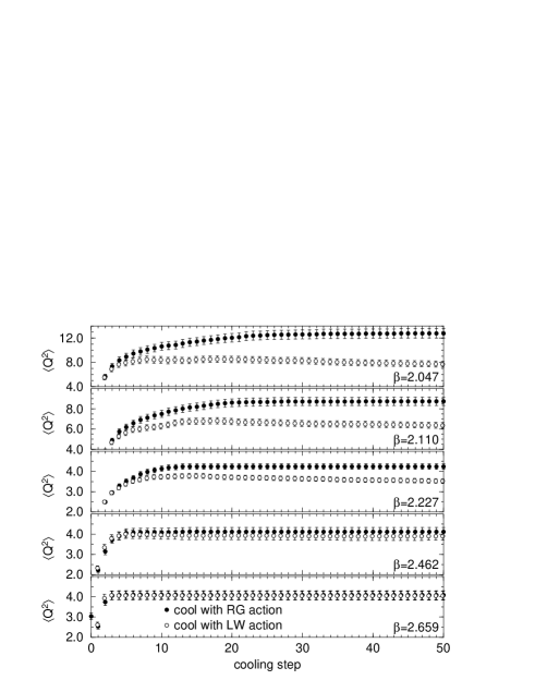
FIG. 2.: Expectation value of the topological charge squared as a function of the number of cooling steps for two different cooling actions.

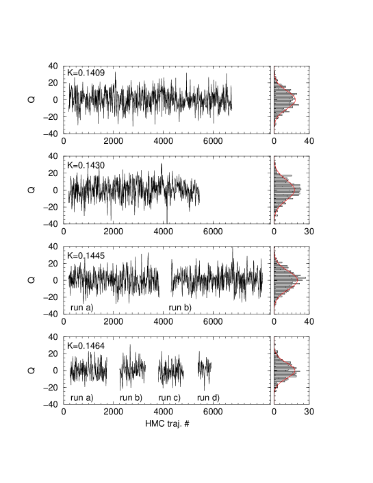
FIG. 3.: Time histories and histograms in full QCD at $\beta=1.80$.

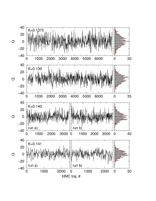
FIG. 4.: Time histories and histograms in full QCD at $\beta=1.95$.

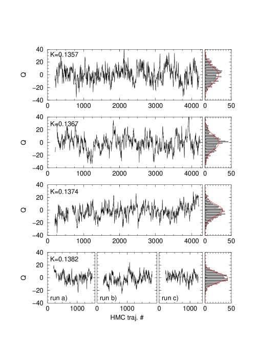
FIG. 5.: Time histories and histograms in full QCD at $\beta=2.10$.

FIG. 6.: String tension in pure SU(3) gauge theory as a function of the gauge coupling. Circles represent data from Refs. [14, 33, 34] while squares are obtained in the present work. The solid line represents a fit with Eq. (18).

     

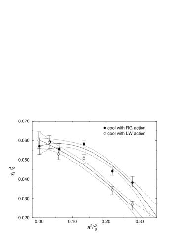
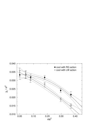
FIG. 7.: Continuum extrapolation of the topological susceptibility in pure SU(3) gauge theory.

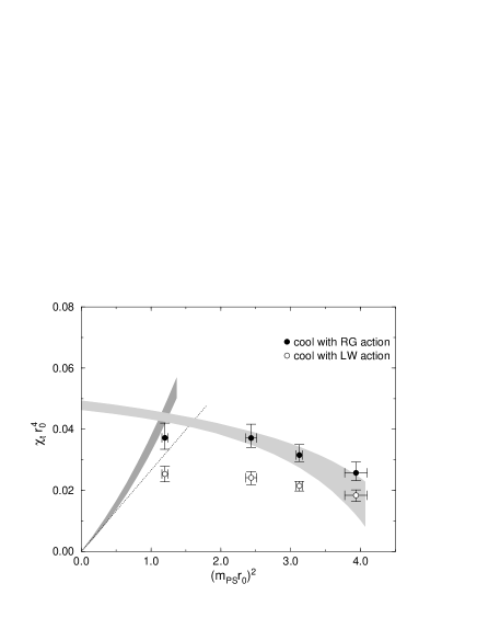
FIG. 8.: Topological susceptibility in full QCD at $\beta=1.80$. The light shaded region indicates the one standard deviation error band for pure SU(3) gauge theory, cooled with the RG-improved action, at corresponding values of $r_{0}$. The darker shaded region starting at zero is the one standard deviation error band of the small mass prediction of Eq. (26) evaluated with measured values of $f_{\rm PS}(m_{\rm PS}^{2})$ and $r_{0}(m_{\rm PS}^{2})$ while the dotted line is the same prediction evaluated with measured values of $f_{\rm PS}$ and $r_{0}$ at physical quark masses.

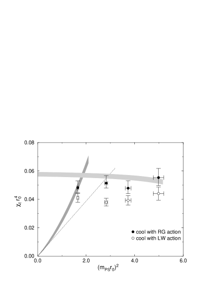
FIG. 9.: Topological susceptibility in full QCD at $\beta=1.95$. Symbols are the same as in Fig. 8.

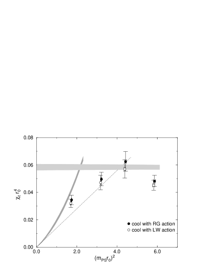
FIG. 10.: Topological susceptibility in full QCD at $\beta=2.10$. Symbols are the same as in Fig. 8.