Oxford OUTP-01-17P

SU(N) gauge theories in four dimensions :
exploring the approach to ${\bf N=\infty}$

B. Lucini and M. Teper

Theoretical Physics, University of Oxford, 1 Keble Road,
Oxford OX1 3NP, UK

Abstract.

We calculate the string tension, $\sigma$, and some of the lightest glueball masses, $m_{G}$, in 3+1 dimensional SU($N$) lattice gauge theories for $2\leq N\leq 5$. From the continuum extrapolation of the lattice values, we find that the mass ratios $m_{G}/\sqrt{\sigma}$ appear to show a rapid approach to the large–$N$ limit, and, indeed, can be described all the way down to SU(2) using just a leading $O(1/N^{2})$ correction. We confirm that the smooth large–$N$ limit we find, is obtained by keeping a constant ’t Hooft coupling. We also calculate the topological charge of the gauge fields. We observe that, as expected, the density of small-size instantons vanishes rapidly as $N$ increases, while the topological susceptibility appears to have a non-zero $N=\infty$ limit.

1 Introduction

How SU($N$) gauge theories approach their $N=\infty$ limit, and what that limit is, is an interesting question [1] whose answer would represent a significant step towards addressing the same question in the context of QCD. Accurate lattice calculations in 2+1 dimensions [2] show that in that case the approach is remarkably precocious in that even $N=2$ is close to $N=\infty$. Such calculations have to be very accurate, of course, because for each value of $N$ one has to perform a continuum extrapolation of various mass ratios and then these are compared and extrapolated to $N=\infty$. Existing D=3+1 calculations [3, 4, 5] are much too rough for this purpose even if their message appears to be optimistic.

In this paper we present a calculation in 3+1 dimensions that is accurate enough for some conclusions to be drawn. This calculation is intended as an exploratory one, designed to see if a much more detailed and extensive calculation is warranted. For this reason we have limited ourselves to calculating just three masses in the (‘glueball’) spectrum: the lightest and first excited $J^{PC}=0^{++}$ scalars, and the lightest $2^{++}$ tensor. We have also calculated the topological susceptibility and have obtained some information on the distribution of ‘instanton’ sizes so as to see how it evolves at larger $N$. We simultaneously investigate linear confinement, calculating the string tension. We do all this for SU(4) and SU(5) gauge theories and compare the results to what one finds for SU(2) and SU(3). In fact, because the existing SU(2) calculations proved too inaccurate to be useful, we found that we had to redo SU(2) as well. We have also chosen to perform our own SU(3) calculations (although this was not absolutely necessary) so that when we compare results at various $N$ in this paper, they will have all been obtained with exactly the same methods.

For $N>3$ there are, in addition, new stable strings that connect sources in representations higher than the fundamental and we have calculated their string tensions. In [6] we presented our preliminary results on this topic. We have since somewhat increased the accuracy of those calculations as well as performing some similar, but much more accurate, calculations in D=2+1. We do not include these calculations in the present paper since they do not really belong to the question being addressed here, i.e. the approach of SU($N$) gauge theories to their $N=\infty$ limit. Instead we will present them elsewhere [7], as this will enable us to present in some detail the theoretical background to the ideas involved. Here we simply remark that our previous conclusions [6] remain unchanged: in the D=3+1 SU(4) and SU(5) gauge theories the doubly charged string has a tension that is much less than twice that of the fundamental string, and it agrees, within fairly small errors, with the M(-theory)QCD conjecture made in [8]. However, as we show in [7] our results also agree with old speculations about the ‘Casimir scaling’ of strings, a dependence that is manifested in leading-order Hamiltonian strong-coupling and which happens to be numerically quite close to the MQCD conjecture. This aspect was not discussed in [6] but is explored in detail in [7]. Interest in Casimir scaling has recently revived [9, 10, 11] following recent studies of unstable higher representation strings in SU(3) [9, 10]. In our much more accurate D=2+1 calculations it is clear that these new stable string tensions, while being close to the MQCD conjecture, do in fact deviate from it. What we see is closer to Casimir scaling although here too the agreement does not appear to be perfect. (Although there is some sign that the deviations disappear quite rapidly with increasing $N$.) The fact that the strings we deal with are stable removes ambiguities in interpreting string tensions of the unstable SU(3) strings and brings into sharp focus the possible relevance of Casimir scaling to the dynamics of confinement [7].

In the next section we summarise the technical details of our lattice calculations. We then study the strong-to-weak coupling transition in the case of SU(4). The practical reason for doing this is to demonstrate that the range of lattice spacings we shall use for our continuum extrapolation avoids this potential phase transition. However the nature of this transition is of interest in itself and it becomes more interesting as $N$ increases. We discuss this in some detail. In Section 4 we present our results on glueball masses and the string tension in SU(2), SU(3), SU(4) and SU(5) gauge theories. We perform the continuum extrapolation of various mass ratios, compare their $N$-dependence and perform an extrapolation to $N=\infty$. We discuss what needs to be done better in future calculations. In Section 5 we ask whether our non-perturbative calculations support the usual diagrammatic expectation [1] that a smooth large-$N$ limit is obtained by keeping the ’t Hooft coupling $\lambda\equiv g^{2}N$ constant. We then turn to calculations of the topological susceptibility and of the size distribution of the topological charges, with a view to clarifying the fate of topological fluctuations as $N$ increases. We finish with some concluding remarks.

We remark that a quite similar calculation of the physical properties of D=3+1 SU($N$) gauge theories is being carried out simultaneously elsewhere [12].

2 Lattice preliminaries

Our four dimensional lattice is hypercubic and has periodic boundary conditions. The degrees of freedom are SU($N$) matrices, $U_{l}$, residing on the links, $l$, of the lattice. In the partition function the fields are weighted with $\exp\{S\}$ where $S$ is the standard plaquette action

$$S=-\beta\sum_{p}\biggl{(}1-{1\over N}ReTr\,U_{p}\biggr{)},$$ (1)

i.e. $U_{p}$ is the ordered product of the matrices on the boundary of the plaquette $p$. For smooth fields this action reduces to the usual continuum action with $\beta=2N/g^{2}$. By varying the inverse lattice coupling $\beta$ we vary the lattice spacing $a$.

Our Monte Carlo mixes standard heat-bath and over-relaxation steps in the ratio $1:4$. These are implemented by updating SU(2) subgroups using the Cabibbo-Marinari prescription [13]. We use 3 subgroups in the case of SU(3), 6 for SU(4) and 10 for SU(5). As a check of efficient ergodicity we use the same algorithm to minimise the action and we find that with this number of subgroups the SU($N$) lattice action does decrease more-or-less as effectively as in the SU(2) gauge theory.

Our typical lattice calculation, at a given value of $\beta$ and for a given volume, involves $10^{5}$ Monte Carlo sweeps through the lattice. (For some of the coarser lattice spacings, where the correlation functions decrease most rapidly, we perform more sweeps.) We perform calculations of correlation functions every 5’th such sweep. Calculations of the topological charge (whose details we leave to Section 6.1) are performed every 50 sweeps.

We calculate correlations of gauge-invariant operators $\phi(t)$, which depend on field variables within a given time-slice, $t$. The basic component of such an operator will typically be the (traced) ordered product of the $U_{l}$ matrices around some closed contour $c$. A contractible contour, such as the plaquette itself, is used for glueball operators. A non-contractible closed contour, which winds around the spatial hyper-torus, projects onto winding strings of fundamental flux. In the confining phase the theory is invariant under a class of centre transformations that ensure that the overlap between such contractible and non-contractible operators is exactly zero. For our lattice action the correlation function of such an operator has good positivity properties, i.e. we can write

$$C(t)=\langle\phi^{\dagger}(t)\phi(0)\rangle=\sum_{n}|\langle\Omega|\phi|n\rangle|^{2}\exp\{-E_{n}t\}$$ (2)

where $|n\rangle$ are the energy eigenstates, with $E_{n}$ the corresponding energies, and $|\Omega\rangle$ is the vacuum state. If the operator has $\langle\phi\rangle=0$ then the vacuum will not contribute to this sum and we can extract the mass of the lightest state with the quantum numbers of $\phi$, from the large-$t$ exponential decay of $C(t)$. To make the mass calculation more efficient we use ${\vec{p}}=0$ operators. Note that on a lattice of lattice spacing $a$ we will have $t=an_{t}$, where $n_{t}$ is an integer labelling the time-slices, so that what we actually obtain from eqn(2) is $aE_{n}$, the energy in lattice units.

In practice a calculation using the simplest lattice string operator is inefficient because the overlap onto the lightest string state is small and so one has to go to large values of $t$ before the contribution of excited states has died away; and there the signal disappears into the statistical noise. There are standard methods [14] for curing this problem, using blocked (smeared) link operators and variational techniques. This is described in detail in, for example, [2]. In this exploratory study we use the simplest blocking technique [2] to produce blocked link matrices, and we form operators by multiplying these blocked links around $1\times 1$ and $1\times 2$ contours. We take linear combinations which transform according to the cubic $A^{++}_{1}$ and $E^{++}$ representations, and this allows us to extract $J^{PC}=0^{++}$ and $J^{PC}=2^{++}$ masses. To make the calculation more efficient we use a variational criterion that determines the linear combination of our operators that has the best overlap onto the lightest $0^{++}$ and $2^{++}$ glueball states, and onto the first excited $0^{++}$ state. These standard techniques are described, for example, in [2].

For any given state we determine the best operator as described above. We then attempt to fit the corresponding correlation function, normalised so that $C(t=0)=1$, with a single exponential in $t$. (Actually a $\cosh$ to take into account the temporal periodicity.) We choose fitting intervals $[t_{1},t_{2}]$ where initially $t_{1}$ is chosen to be $t_{1}=0$ and then is increased until an acceptable fit is achieved. The value of $t_{2}$ is chosen so that there are at least 3, and preferably 4, values of $t$ being fitted. (Since our fitting function has two parameters.) Where $t_{1}=0$ and the errors on $C(t=a)$ are much smaller than the errors at $t\geq 2a$, this procedure provides no significant evidence for the validity of the exponential fit, and so we use the much larger error from $C(t=2a)$ rather than $C(t=a)$. (This typically arises on the coarsest lattices and/or for very massive states.) We ignore correlations between statistical errors at different $t$ and attempt to compensate for this both by demanding a lower $\chi^{2}$ for the best acceptable fit and by not extending unnecessarily the fitting range. (Although in practice the error on the best fit increases as we increase the fitting range, presumably because the correlation in $t$ of the errors is modest and the decorrelation of the operator correlations is less efficient as $t$ increases.) The relatively rough temporal discretisation of many of our calculations, means that, at the margins, there are inevitable ambiguities in this procedure. These however decrease as $a\to 0$. Once a fitting range is chosen, the error on the mass is obtained by a Jack-knife procedure which deals correctly with any error correlations as long as the binned data are statistically independent. Typically we take 50 bins, each involving some 2000 sweeps. It is plausible that bins of this size are independent; however we have not stored our results in a sufficiently differential form that we can calculate the autocorrelation functions so as to test this in detail. A crude test is provided by recalculating the statistical errors using bins that are twice as large. We find the errors are essentially unchanged, which provides some evidence for the statistical independence of our original bins.

3 The strong–to–weak coupling transition

It has long been known that if we use the standard plaquette action then we find a cross-over between the strong and weak coupling regions, which is characterised by an anomalous dip in the mass of the lightest scalar glueball and a peak in the specific heat. This effect becomes more marked as we go from SU(2) to SU(3) and it is believed that in the case of SU($N\geq 4$) one has an actual bulk phase transition in this cross-over region. We want to locate the crossover to make sure that it does not interfere with our continuum extrapolations. We shall do so for the case of SU(4) where there have been rough estimates [3] that it is located in the region $\beta\in[10.3,10.5]$.

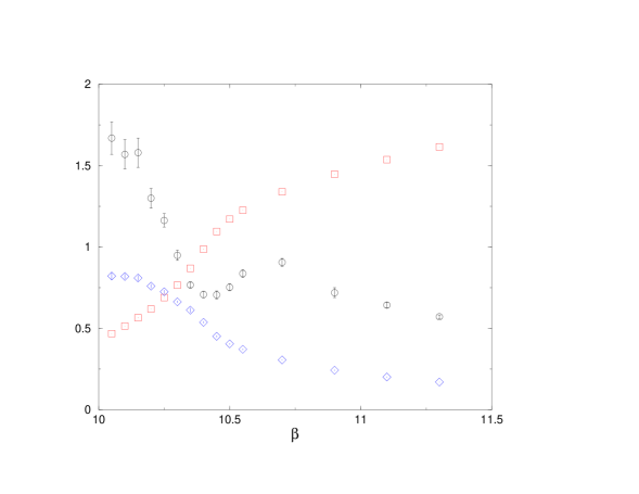
Figure 1: The (rescaled) average plaquette, $\Box$, the mass gap, $\circ$, and the square root of the string tension, $\Diamond$, over a range of $\beta$ that includes the region of transition between strong and weak coupling, for the SU(4) gauge theory.

To locate the cross-over region we calculate the lightest scalar glueball mass, the string tension and the plaquette, in the range of couplings $\beta\in[10.0,11.3]$. Since we think of the lattice spacing as increasing with $\beta$ we would naively expect the value of $am$, for any mass $m$, to decrease uniformly over this range. And indeed, as we see in Fig.1, this is the case for the square root of the string tension, $a\surd\sigma$. However, as we see in Fig.1, this is not the case for the lightest scalar glueball, $am_{0^{++}}$, which has a striking dip at $\beta\sim 10.4$. We note that in this region the value of $ds/d\beta$, where $s$ is the average plaquette, has a maximum, which tells us that there will be a peak in the specific heat here. Taking into account that the dip in $am_{0^{++}}$ is superimposed on a montonically decreasing function, we estimate that the crossover is centered somewhere in $\beta\in[10.35,10.40]$. The calculations we shall use to extrapolate to the continuum limit will all be well to the weak-coupling side of this value of $\beta$.

As far as the presence of an actual phase transition is concerned, we see no sign of a strong first order transition in that there appear to be no discontinuities in any of the quantities we calculate. We have not done the kind of finite volume study that might reveal a second order transition; although at $\beta=10.30$, where we have calculations on two volumes, there is no sign of the dip becoming deeper as the volume increases. But we emphasise that our calculations were not designed to locate a phase transition, and instead were merely intended to identify the cross-over region.

Several reasons have been given in the past for a crossover or phase transition separating the strong and weak coupling regimes in SU($N$) gauge theories. One explanation focuses on string roughening (see [15, 16] and references therein): in strong coupling the confining string is rigid, as though the transverse fluctuations were massive, while in weak coupling we recover the usual continuum-like string with massless transverse fluctuations. In the region of couplings where this mass vanishes the string becomes rough and the lattice theory should exhibit a cross-over [15, 16]. A quite different approach [17] focuses on the different eigenvalue distributions that the plaquette matrix possesses at strong and weak coupling. From this one can conclude [17] that there is a third-order phase transition separating the strong and weak coupling regions at $N=\infty$ with, presumably, some kind of cross-over at finite but large $N$. A third approach [18, 16] focuses on the phase structure in an extended coupling space, driven by the condensation of various lattice topological objects [19, 20]. We will now comment on, and extend a little further, this last idea.

We start by considering SU(2). Suppose one generalises the lattice action in eqn(1) to

$$S=-\beta\sum_{p}\biggl{(}1-{1\over N}ReTr\,U_{p}\biggr{)}-\beta_{A}\sum_{p}\biggl{(}1-{1\over{N^{2}-1}}ReTr_{A}\,U_{p}\biggr{)},$$ (3)

where $Tr_{A}$ is the trace in the adjoint representation, and the $Tr$ in the first term continues to be in the fundamental representation. This lattice theory has a non-trivial phase structure in the $(\beta,\beta_{A})$ space of couplings [18, 16]. In particular there is a phase transition line which ends in a critical point and this point approaches the Wilson axis, $\beta_{A}=0$, as we go from SU(2) to SU(3). Moreover if one extrapolates this phase transition line one crosses the Wilson axis in the weak-to-strong coupling crossover region. Since the mass gap vanishes at the critical point, its proximity to the Wilson axis provides an explanation for the dip in the mass of the scalar glueball in the region that characterises the transition from weak to strong coupling, and also the fact that this dip deepens as we go from SU(2) to SU(3).

The SU(2) phase structure described above is believed to be driven by the following dynamics [19, 20]. If we multiply a link matrix by an element of the centre then this is invisible to the adjoint piece of the action. Strings of plaquettes of flipped sign can be thought of as $Z_{2}$ vortex lines. Such vortices may be closed or may end on $Z_{2}$ monopoles. At small $\beta$ and small $\beta_{A}$ there will be a vacuum condensate of both the $Z_{2}$ vortices and the $Z_{2}$ monopoles. If we increase $\beta_{A}$ at $\beta\sim 0$ the vortices remain condensed since the adjoint action does not feel their presence. However the monopoles will cease to condense at some critical value of the coupling for the same entropy/action reason that U(1) monopoles cease to be condensed in the D=3+1 U(1) theory beyond a certain critical coupling. Thus there is a phase transition line extending to finite $\beta$ from some point along the adjoint axis. Now if we go to large $\beta_{A}$ the plaquettes are all close to $\pm 1$ and we have something close to a $Z_{2}$ spin system. If we then increase $\beta$ this is equivalent to increasing an external field that breaks the $Z_{2}$ symmetry and at some point there is a phase transition to a phase where the (ultraviolet) $Z_{2}$ vortices are suppressed. So there is a phase transition line descending into the $(\beta,\beta_{A})$ plane. At some point this coalesces with the other phase transition line and continues downwards till it ends at the critical point. That it must end somewhere follows from the fact that at large negative $\beta_{A}$ the plaquette traces are driven close to zero, and such a vacuum will support neither $Z_{2}$ vortices nor monopoles.

We note that although this kind of explanation sounds very particular to the simple plaquette action, one should be able to generalise it to any loops; the crucial thing is that we consider them in both the fundamental and adjoint representations. One might wonder whether other representations might be relevant. It is clear however that the relevant topological objects are determined by the centre of the group and a loop in any SU(2) representation responds either like the fundamental or adjoint representation to centre elements of the group. Thus the analysis possesses a qualitative universality.

In SU(3) the picture is essentially the same, but if we go to SU(4) things become different. Now we can introduce an extra $k=2$ coupling, $\beta_{2}$, corresponding to double flux plaquettes. Such plaquettes are insensitive to a factor $e^{i\pi}=-1$, just like the adjoint coupling. However the adjoint action is also insensitive to $e^{i\pi/2}$ fluxes. By the above kind of argument we expect a similar phase structure in the SU(4) $(\beta,\beta_{k=2})$ plane to the one we had in the SU(2) $(\beta,\beta_{A})$ plane. Indeed we should now consider the $(\beta,\beta_{k=2},\beta_{A})$ manifold of couplings, and there will be surfaces of phase transitions and lines of critical points which may approach the Wilson axis at more than one location. For higher SU($N$) we have a $(\beta,\beta_{2},\beta_{3},\ldots,\beta_{A})$ space of couplings where the different pieces of the action will be insensitive to different elements of the centre. That is to say, to monopoles and vortices of various multiples of the basic $Z_{N}$ flux. There will be a complex phase structure in this space, but since it involves the condensation of ultraviolet objects, one can in principle estimate the location of these transitions. We do not attempt to do so here. However we point out that these phase transitions would naturally be related to the eigenvalue spectrum of the typical SU($N$) plaquette. It is not unreasonable to conjecture that the smooth $N\to\infty$ limit of this complex phase structure might be precisely the third-order phase transition discussed in [17].

Finally we remark that there is no sign of a cross-over, marked by a dip in the mass gap, when we consider SU($N$) gauge theories in D=2+1. Since the vacuum possesses all the topological objects described above, this might look like a counterexample to the argument. In fact this is not so. The key observation is that in the D=2+1 U(1) theory there is no phase transition between strong and weak coupling: in contrast to the D=3+1 case. This is because in D=2+1 the monopoles are instantons, while in D=3+1 they are objects with world lines. Thus the action/entropy balance is quite different and leads to a quite different phase structure. This applies equally well to $Z_{N}$ monopoles.

4 The spectrum and string tension

In Sections 4.1 and 4.2 we describe our calculations of the string tension and of the mass spectrum respectively. We then discuss, in Section 4.3, what are the lessons we learn as to how to go about doing a much better calculation.

4.1 the string tension

To calculate the (fundamental) string tension $\sigma$ we construct string operators that close upon themselves through a spatial boundary. The correlation function of two such strings separated by a (Euclidean) time interval $t$ will, for large enough $t$, decrease exponentially $\propto\exp(-m_{l}t)$ where $m_{l}$ is the mass of the lightest periodic flux loop. On the lattice $t=an_{t}$ where $n_{t}$ labels the temporal time-slices, so what we obtain is the value of $am_{l}$, the mass in lattice units. If the length of the loop is $aL$ and if the theory is linearly confining then $a^{2}\sigma=\lim_{L\to\infty}am_{l}/L$. Moreover the first correction to this linear dependence is universal [21] if the infrared properties of the confining flux tube are described by an effective string theory. If we further assume that the universality class is that of a simple (Nambu-Gotto) bosonic string (there is some evidence from previous SU(2) and SU(3) lattice calculations that points to this) and if we use the string correction appropriate to our closed periodic string [22] then we find

$$am_{l}=a^{2}\sigma L-\frac{\pi}{3L}$$ (4)

once the flux loop is large enough. We shall use this expression to extract $a^{2}\sigma$ from our lattice calculations of the flux loop mass $am_{l}$.

As we have just remarked, in using eqn(4) we are assuming that we have linear confinement in our $SU(N)$ gauge theories, that the effective string theory describing the infrared properties of the confining flux tube is in the Nambu-Gotto universality class, and that our string is in fact long enough for higher order corrections to be negligible. There is, of course, a great deal of numerical evidence, scattered through the literature, for linear confinement in the case of SU(2) and SU(3) as well as some (much weaker) evidence that the leading correction is as in eqn(4). To address these issues for $SU(N>3)$ we show in Fig.2 how the value of $am_{l}$ varies with $L$ in SU(4) at a particular value of $a$. In Fig.3 we perform a similar exercise for the case of SU(3). We observe that for SU(4), just as for SU(3), the mass $am_{l}$ increases roughly linearly with $L$: evidence for linear confinement. We also note that in both cases the deviation from linearity is consistent with eqn(4) for the largest two values of $L$ and that in both cases this occurs for distances $aL\geq 3/\surd\sigma$. If we equate the masses corresponding to these longest two loops to $am_{l}=bL-c/L$ then we find $c=0.94\pm 0.41$ and $c=0.76\pm 0.43$ for the SU(3) and SU(4) cases respectively. These values are consistent with the value $c=\pi/3\simeq 1.05$ assumed in eqn(4). We emphasise that, with only two values of $L$ fitting this correction, we cannot claim to have evidence for both the $1/L$ functional form and for its coefficient. Rather we can say that if we assume the functional form then we have some evidence that the bosonic string coefficient, as in eqn(4), is the correct one. This is thus a minimal finite size study (which we are in the process of improving upon [7]) but it does indicate that it should be safe, within our statistical accuracy, to use eqn(4) to extract $a^{2}\sigma$ as long as we do so for $aL\geq 3/\surd\sigma$.

We remark that although our determination of the string correction is not very precise, using periodic loops rather than Wilson loops is by far the better way to approach this question. One reason is that the string correction has a larger coefficient in the former case; $c=\pi/3$ as compared to $c=\pi/12$ for Wilson loops. More importantly, with Wilson loops the string is attached to static sources which provide a Coulomb interaction. This has the same functional form as the string correction and dominates the potential at shorter distances. Thus in fits to the potential of the form $V(r)=v+\sigma r+c/r$ the value of $c$ will be dominated by the short-distance Coulomb interaction rather than the long-distance string correction, unless one confines the fitting range to distances greater than, say, 1 fm. (Indeed, as we have seen, the periodic flux loop has to have a length $r\geq 3/\surd\sigma\simeq 1.3fm$ if the leading string correction is to dominate.) This is a tough criterion for Wilson loop calculations and is rarely met.

The loop masses and string tensions obtained in our SU(2), SU(3), SU(4) and SU(5) lattice calculations are listed in Tables 1, 2, 3 and 4 respectively. In the various continuum extrapolations that we shall perform we shall only use string tensions calculated on lattices that satisfy $aL\geq 3/\surd\sigma$ and thus ones to which we believe the application of eqn(4) is justified.

4.2 the mass spectrum

In addition to the string tension, we calculate the masses of the lightest scalar and tensor glueballs, as well as the mass of the first scalar excitation. These are obtained from correlations of operators that are obtained by multiplying link matrices around closed contractible loops. These masses are listed in Tables 1, 2, 3 and 4.

The first question to ask is how large the spatial volume has to be for glueball finite volume corrections to be negligible (at our level of statistical accuracy). To answer this question we have performed mass calculations on a range of lattice volumes at $\beta=10.7$ in the case of SU(4) and at $\beta=5.93$ in the case of SU(3). The masses are listed in Tables 3 and 2 respectively. We observe that the lightest $J^{PC}=0^{++}$ and $2^{++}$ glueballs appear to have reached (within errors) their infinite volume limit once $aL\surd\sigma\geq 3$. For the excited $0^{++\star}$ scalar the situation is less clear: it appears to be the case for SU(4) but apparently not for SU(3). We shall return to the probable cause of this in Section 4.3 but for now we shall simply assume that it is safe to calculate glueball masses and the string tension on lattice volumes that satisfy the constraint $L\geq 3/a\surd\sigma$.

We are interested in determining the $N$ dependence of physical quantities in the continuum limit. We first note that if we form a dimensionless ratio of physical quantities then the lattice scale drops out, e.g. $am_{G}/a\surd\sigma\equiv m_{G}/\surd\sigma$. This ratio will of course still possess lattice corrections. However the functional form of such corrections is known. In particular for our simple plaquette action we expect the leading correction to be $O(a^{2})$. Thus for small enough $a$ we expect the continuum limit to be approached as

$${{m_{G}(a)}\over{\surd\sigma(a)}}={{m_{G}(0)}\over{\surd\sigma(0)}}+ca^{2}\sigma.$$ (5)

We could use any mass $\mu$ in the correction term, since $a^{2}\sigma$ and $a^{2}\mu^{2}$ differ at $O(a^{4})$. We choose to use $\sigma$ both for the correction term and in our dimensionless mass ratios, because it is the quantity we calculate most accurately and reliably. (In reality $c$ in eqn(5) is a power series in $g^{2}(a)$. However, since the logarithmic variation of the coupling is very small over our range of $a$, we follow usual practice and treat it as a constant.)

Our procedure is therefore to fit our lattice ratios with eqn(5). We begin by including all our calculated values. If the best fit is poor, we drop the coarsest value of $a$ and re-attempt the fit – and so on. Following this procedure we obtain the continuum mass ratios listed in Table 5. We remark that the SU(2) and SU(3) values agree with those obtained previously, as reviewed for example in [4], and that our SU(2) mass ratios are much more accurate than earlier work, as expected.

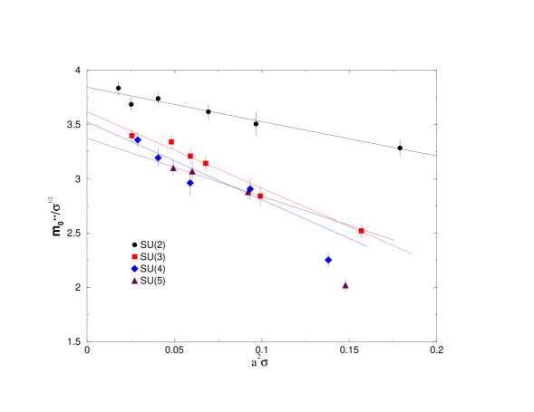
Figure 4: The mass of the lightest scalar glueball, $m_{0^{++}}$, expressed in units of the string tension, $\sigma$, is plotted against the latter in lattice units. The continuum extrapolation, using a leading lattice correction, is shown.

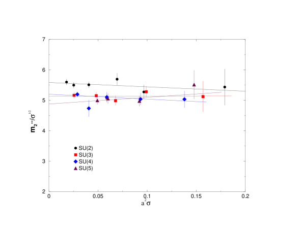
Figure 5: The mass of the lightest tensor glueball, $m_{2^{++}}$, expressed in units of the string tension, $\sigma$, is plotted against the latter in lattice units. The continuum extrapolation, using a leading lattice correction, is shown.

The best fits involved in the extrapolations of the lightest $0^{++}$ and $2^{++}$ glueballs are almost always very good, and in any case never poor. They are shown, together with the lattice ratios, in Fig.4 and Fig.5. We note the increasing influence as $N$ increases of the strong-to-weak coupling crossover on the mass of the $0^{++}$ at the coarsest lattice spacing. For SU(5) the $0^{++\star}$ fit is also good, and for SU(2) it is at least acceptable. However for SU(3) and SU(4) the best fits are very poor. In these cases we have quoted generous errors in an attempt not to be misleading. We believe we understand the origin of these problems with the $0^{++\star}$, and this is discussed in Section 4.3.

We are now in a position to discuss the $N$ dependence of continuum SU($N$) gauge theories. We expect that once $N$ is large enough, mass ratios will have a smooth limit with a leading correction that is $O(1/N^{2})$, i.e.

$$\left.{{m_{G}}\over{\surd\sigma}}\right|_{N}=\left.{{m_{G}}\over{\surd\sigma}}\right|_{\infty}+{c\over N^{2}}.$$ (6)

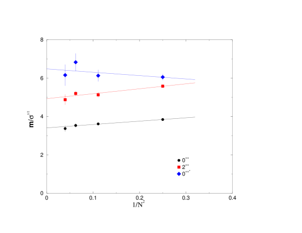
Figure 6: Continuum scalar, tensor and excited scalar masses expressed in units of the string tension and plotted against $1/N^{2}$. Linear extrapolations to $N=\infty$ are shown in each case.

In Fig.6 we plot the continuum mass ratios against $1/N^{2}$. According to eqn.(6) once $N$ is sufficiently close to $N=\infty$ the mass ratios should fall on a straight line. Performing linear fits we observe that in fact this is the case all the way down to $N=2$. For the $0^{++\star}$ this is perhaps not so significant because the errors are so large; however in the case of the $2^{++}$ and of the $0^{++}$ the errors are small and the result is striking.

Our best fits for $N\geq 2$ are:

$${{m_{0^{++}}}\over{\surd\sigma}}=3.37(15)+{{1.93(85)}\over N^{2}}$$ (7)

$${{m_{2^{++}}}\over{\surd\sigma}}=4.93(30)+{{2.6(1.9)}\over N^{2}}$$ (8)

and

$${{m_{0^{++\star}}}\over{\surd\sigma}}=6.43(50)-{{1.5(2.6)}\over N^{2}}$$ (9)

These relations give us the corresponding mass ratios not only for $N=\infty$ but for all values of $N$. The fact that we can fit these mass ratios with just the leading $1/N^{2}$ corrections all the way down to $N=2$ and the fact that the coefficients are quite small can be summarised by saying that all SU($N$) gauge theories are close to SU($\infty$), at least as far as the low-lying mass spectrum is concerned.

4.3 discussion

Our above results provide a clear motivation for a much more detailed calculation. From what we have learned here, how should such a calculation proceed?

We have seen that there is a large gap to the first excited scalar state. The lesson is that if we want a detailed mass spectrum, many of the states will be quite heavy in lattice units. In this situation the best strategy is to use an anisotropic lattice with a fine temporal lattice spacing that allows a much finer resolution of the rapidly decreasing correlation functions that correspond to heavy masses. This is an idea and technique with a long history [23] which has been used to impressive effect in recent calculations of the SU(3) mass spectrum [24] (and also in calculations of the static potential [10]).

The first excited scalar has a mass $m_{0^{++\star}}\simeq 2m_{0^{++}}$. This raises the question whether it might not in fact be a two glueball scattering state with zero relative momentum. Within our present calculation we cannot answer this question with any certainty. Any future calculation should include in the variational basis of operators explicit multi-glueball operators for all the scattering states, of various relative momenta, that are expected to lie in the mass range of interest. In this way we can hope to identify and separate bound states or resonances from the less interesting scattering states.

In addition to any bound states, resonances and scattering states, there are also extra states which decouple in the infinite volume limit but which are not so heavy that they can be ignored for the kind of volumes we are likely to use. These ‘torelon’ states (see [2] and references therein), which are composed of a periodic flux loop and its conjugate, have a mass that is about twice the mass of the single flux loop: $m_{T}\simeq 2m_{l}$. This mass increases roughly linearly with the volume of course, but for much of the present calculations this happens to be close to $m_{0^{++\star}}$. Indeed the strong finite-size effects we observe $m_{0^{++\star}}$ to possess in our SU(3) study, suggests an occasional misidentification with such a torelon state. In the case of SU(3) and SU(4) the volumes are less constant than in the case of SU(2) which suggests this as the reason for the poor continuum extrapolation. Again the solution to the problem is to include explicit torelon operators in the variational basis so as to make the explicit identification of these states possible.

The above discussion should however not be taken to imply that we have no faith in our estimate of the excited scalar mass. The reason is that our glueball operators involve the trace of a single loop, and we expect the overlap of both the torelon and two-glueball states on such operators to decrease rapidly with increasing $N$. Thus we are inclined to believe that what we observe in SU(5) is a genuine excited glueball state, so that our large-$N$ mass estimate should be quite reliable.

Our second observation, based on our tabulated masses, is that the errors on the masses appear to increase as we go from SU(2) to larger $N$. This could be a problem that is intrinsic to such a calculation. One possible reason is that, as we shall see below, the sampling of different vacuum topological sectors becomes rapidly less ergodic as $N$ increases. Another reason is that as $N$ grows the path integral is increasingly dominated by the single ‘Master Field’ [1]. Our mass calculations are derived from the correlations in distant fluctuations about this Master Field and perhaps this method becomes inefficient at large $N$. (In which case it is an interesting question to ask how one might calculate the masses.) Because of its practical importance we have investigated this question in detail. What we find is that the actual correlation functions do not display statistical errors that grow with $N$. This is good news: it means that the problem is not an intrinsic one. What happens is that our best operators have a poorer overlap onto the lightest states as $N$ increases. This is more pronounced for the flux loop than for the glueballs, and becomes more pronounced at smaller $a$ in the latter case. It may be useful to illustrate this with some explicit values. Consider the overlap that appears in eqn(2), $c^{2}_{n}\equiv|\langle\Omega|\phi|n\rangle|^{2}$, where we normalise $\sum_{n}c^{2}_{n}=1$. For the best $0^{++}$ glueball operator the value of $c^{2}_{n}$ varies, for our coarsest common value of $a$, from $\sim 0.95$ in SU(2) to $\sim 0.90$ in SU(5). For the finest (common) values of $a$ it varies from $\sim 0.92$ to $\sim 0.85$. For the periodic flux loop the corresponding variation of $c^{2}_{n}$ is from $\sim 0.90$ to $\sim 0.75$ for both coarse and fine values of $a$. This behaviour suggests that the problem is with our simple blocking algorithm. A better strategy would be to intermingle smearing and blocking steps. In any case the lesson here is that a much better calculation will require the construction of operators with better overlaps.

Another important issue concerns quantum numbers. Typically our operators fall into representations of the cubic group. What we have called $0^{++}$ is actually the cubic $A^{++}_{1}$ representation which also includes pieces of other continuum representations, such as the $4^{++}$. For the lightest states one can identify criteria [2] which reassure us that our continuum spin labelling is correct. However the ambiguity becomes larger for excited states. For example, one can ask whether our claimed $0^{++\star}$ might not in fact be the lightest $4^{++}$. Since the higher-spin continuum representations are typically spread between several representations of the cubic group, one approach to resolving these ambiguities is to search for corresponding degeneracies between states in different cubic representations. However it is unlikely that one will, in practice, obtain these heavier masses with sufficient accuracy to establish degeneracy unambiguously. (Which, in any case, only becomes exact for small $a$.) An alternative (or additional) strategy is to construct operators with approximate continuum rotational properties [25]. One can then use the size of the overlap of the excited states onto such operators to determine what their likely quantum numbers are.

5 ’t Hooft coupling

The calculations in the previous Section indicate that SU($N$) gauge theories have a smooth limit as $N\to\infty$, that the theory remains confining, and that the approach is ‘precocious’ in the sense that even SU(2) appears to be within a modest $O(1/N^{2})$ correction of SU($\infty$).

The analysis of diagrams [1] suggests that such a smooth limit should be achieved by keeping the ’t Hooft coupling, $\lambda\equiv g^{2}N$, constant as $N\to\infty$. We shall now see to what extent this expectation can be addressed by our calculations.

Since the coupling runs, the ’t Hooft coupling is not a constant but will depend on the length scale $l$ on which it is defined, i.e. $\lambda(l)\equiv g^{2}(l)N$. Thus we expect that if we fix the value of $l$ in units of some quantity that partakes of the smooth large-$N$ limit, such as the string tension, then $\lambda(l)$ should have a smooth non-trivial limit as $N\to\infty$. Now, we can define couplings in various ways, and one way is to use $\beta=2N/g^{2}$. Here $g^{2}$ is the lattice bare coupling and provides a definition of a coupling on the length scale $a$. Thus we define

$$\lambda(a)=g^{2}(a)N=2N^{2}/\beta$$ (10)

However it is well known that in our range of $a$ this coupling is heavily influenced by lattice artifacts peculiar to the plaquette action, and that a much better coupling can be obtained from it by the definition

$$\lambda_{I}(a)=g_{I}^{2}(a)N=2N^{2}/\beta_{I}=2N^{2}/(\beta\times{1\over N}\langle ReTr\,U_{p}\rangle)$$ (11)

which may be regarded as a mean-field improved or tadpole improved version of $\beta$ and $\lambda(a)$ [26].

An aside. Ideally we would have wished to define a coupling on some scale $l\gg a$ so that we could determine its behaviour at fixed $l$ as $a\to 0$ and then compare how this continuum coupling varies with $N$. (For example one might use the coupling definition in [27].) Using $\beta$, as we do, mixes in lattice corrections in an uncontrolled fashion. Transforming this to $\beta_{I}$ is known to remove a large part of the lattice corrections at small $a$. Nonetheless, the fact that these lattice corrections vary with the scale $l$, because of course $l=a$, will limit our ability to probe the interesting question of what happens to the coupling on larger distance scales.

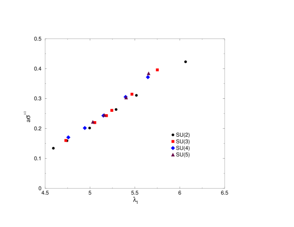
Figure 7: The square root of the string tension in lattice units, $a\surd\sigma$, plotted against the ’t Hooft coupling, $\lambda_{I}\equiv g^{2}_{I}N$.

To test whether we get a smooth large-$N$ limit by keeping $\lambda_{I}(l=a)$ fixed, we need to choose a physical length scale in terms of which we keep $l$ fixed. We shall choose $1/\surd\sigma$ since we have already seen that the ratio of $\surd\sigma$ to other masses has a smooth large-$N$ limit. Thus our first expectation is that if we plot $a\surd\sigma$ against $\lambda_{I}(a)$ then, for large enough $N$, the calculated values should fall on a universal curve. In Fig.7 we plot all our calculated values of $a\surd\sigma$, against the value of $\lambda_{I}(a)$, for $N=2,3,4$ and $5$. We observe that, within corrections which are small except at the largest value of $a$, we do indeed see a universal curve.

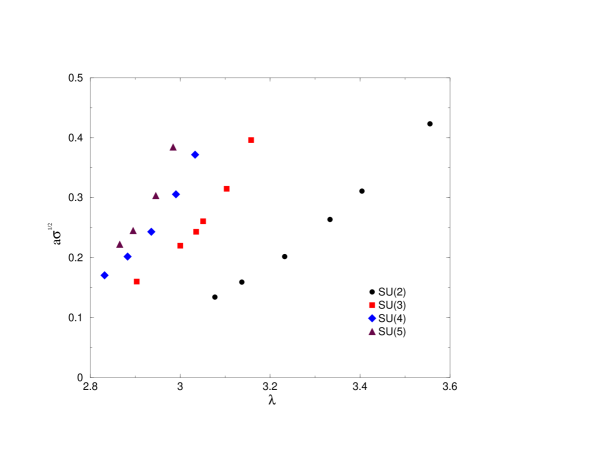
Figure 8: The square root of the string tension in lattice units, $a\surd\sigma$, plotted against the unimproved ’t Hooft coupling, $\lambda\equiv g^{2}N$.

It is instructive to ask what would have happened if we had used eqn(10) rather than eqn(11) to define our running coupling. The answer is displayed in Fig.8. Here we see how very large lattice corrections can easily hide the approach to large-$N$.

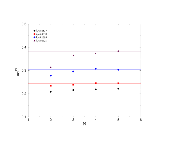
Figure 9: We show how the string tension varies with $N$ at four different values of the ’t Hooft coupling.

While Fig.7 makes the qualitative point, it is hard to make out the details of the approach to the $N=\infty$ limit. To display this we start with each of our four SU(5) values of $\beta$ and calculate the value of $a\surd\sigma$ obtained at the corresponding value of $\lambda_{I}$ for $N=2,3,4,5$. (To obtain these values for $N\not=5$ requires some interpolation.) In Fig.9 we show how the string tension varies with $N$ at these four fixed values of the ’t Hooft coupling. We see that at all values of $a$ except the largest (where we are close to the strong-to-weak coupling crossover) the string tension at fixed ’t Hooft coupling becomes independent of $N$, within our errors, for $N\geq 4$.

Once the coupling $g_{I}^{2}(a)$ is small enough to be accurately given by its 2-loop perturbative formula, we can replace the above analysis by simply extracting the scale $\Lambda_{I}$ that appears in the 2-loop formula for the running coupling, and seeing if it also has a smooth large-$N$ limit. We can use our calculations to illustrate how such an analysis proceeds, even though we do not really expect our couplings to be small enough for it to be very reliable. First we invert the 2-loop formula so as to obtain $a$ in terms of $g^{2}(a)$, and then we multiply both sides by $\surd\sigma$ to obtain

$$a\surd\sigma={{\surd\sigma}\over{\Lambda_{I}}}\biggl{(}{{24\pi^{2}}\over{11}}{{\beta_{I}}\over{N^{2}}}\biggr{)}^{{51}\over{121}}\exp\biggl{(}-{{{12\pi^{2}}\over{11}}{{\beta_{I}}\over{N^{2}}}}\biggr{)}.$$ (12)

which gives us $\Lambda_{I}$ in units of a physical mass scale, $\surd\sigma$, of the SU($N$) gauge theory. Using this formula we can extract a value of $\surd\sigma/\Lambda_{I}$ from each of our lattice calculations of $a\surd\sigma$. This value will receive $O(a^{2})$ corrections in the usual way, but it will also receive $O(g^{2})$ perturbative corrections to the two-loop formula in eqn(12). These corrections will vary by very little over our range of $a$ and we would not be able to determine them numerically. By contrast the $O(a^{2})$ correction varies strongly so we can perform a continuum extrapolation

$${{\surd\sigma(a)}\over{\Lambda^{eff}_{I}(a)}}={{\surd\sigma(0)}\over{\Lambda^{eff}_{I}(0)}}+ca^{2}\sigma$$ (13)

where $\Lambda^{eff}_{I}$ is the value of $\Lambda_{I}$ renormalised by an unknown $1+O(\bar{g^{2}_{I}})$ factor, where $\bar{g^{2}_{I}}$ is the (approximately constant) value of ${g^{2}_{I}}$ in our range of $a$. Performing the continuum extrapolation in eqn(13) we obtain the values shown in Table 6. We note that the best continuum fit is very poor in the case of SU(2), acceptable for SU(3) and good for SU(4) and SU(5). We then find that we obtain a good fit to these values using just the expected leading $O(1/N^{2})$ correction:

$${{\surd\sigma}\over{\Lambda^{eff}_{I}}}=6.05(9)-{{2.65(85)}\over{N^{2}}}.$$ (14)

That is to say, we find that the $\Lambda$ parameter also appears to have a smooth limit as $N\to\infty$. It is perhaps surprising how well this analysis has worked given the fact that our values of $g_{I}^{2}(a)$ are not really that small.

6 Topology and instantons

A Euclidean continuum SU($N$) gauge field on a hypertorus will possess an integer topological charge $Q$. The fluctuations of this charge may be characterised by the topological susceptibility, $\chi_{t}\equiv\langle Q^{2}\rangle/V$, where $V$ is the volume of space-time. In QCD one can argue [28] that these topological fluctuations make the $\eta^{\prime}$ massive and so solve the axial $U(1)$ problem. In the large-$N$ limit fermions decouple (for any non-zero quark mass), so the vacuum topological fluctuations become the same as those of the SU($N$) gauge theory. Thus in QCD at large-$N$ and with $N_{f}$ flavours, one can relate the mass of the $\eta^{\prime}$ to the topological susceptibility of the SU($N$) gauge theory [29]:

$$\chi_{t}\simeq{{m^{2}_{\eta^{\prime}}f^{2}_{\eta^{\prime}}}\over{2N_{f}}}\sim(180\ MeV)^{4}.$$ (15)

To obtain the value as $(180\ MeV)^{4}$ one assumes that corrections to this relation are small for SU(3) so that one can use the experimental values for $m_{\eta^{\prime}}$ and $f_{\eta^{\prime}}$. (One also assumes the latter to be equal to $f_{\pi}$ and one corrects eqn(15) for the small pseudoscalar octet contribution.) There have been many lattice calculations of $\chi_{t}$ in SU(3) intended to test the relation in eqn(15). The comparison turns out to be quite successful (see [30] for a review) but of course it only makes sense if the finite-$N$ corrections are small for SU(3). We are not here in a position to estimate the corrections to the large-$N$ relation $m^{2}_{\eta^{\prime}}\propto 1/N$, but we can check if the SU(3) topological susceptibility is close to its large-$N$ limit, and we shall do so later in this section.

While one hopes that the fluctuations of the topological charge are not going to change a great deal when one goes from $N=3$ to $N=\infty$, the number density of instantons, by contrast, is expected to suffer a strong exponential suppression [31]:

$$D(\rho)\propto e^{-{{8\pi^{2}}\over{g^{2}(\rho)}}}=e^{-{{8\pi^{2}}\over{\lambda(\rho)}}N}$$ (16)

where $\rho$ is the instanton size and $\lambda\equiv g^{2}N$ is the ’t Hooft coupling which is kept constant as $N\to\infty$. At first sight it is hard to see how $\chi_{t}$ can depend weakly on $N$ if the instanton density depends so strongly. One can see how this may be [32] if we include in our expression for $D(\rho)$ the factor that arises from the various ways that an SU(2) subgroup may be embedded in SU($N$):

$$D(\rho)d\rho\propto{{d\rho}\over{\rho}}{1\over{\rho^{4}}}\Biggl{\{}{{b^{2}}\over{\lambda^{2}(\rho)}}e^{-{{8\pi^{2}}\over{\lambda(\rho)}}}\Biggr{\}}^{N}.$$ (17)

Here $b$ is some known constant and we have also included the scale-invariant measure, and volume factor. We see that while at very small $\rho$, where $\lambda(\rho)$ is small, there will indeed be a strong exponential suppression of $D(\rho)$ as $N$ increases, this weakens with increasing $\rho$. At the same time, as $\rho$ increases (anti-)instantons will begin to overlap and the effective action of an instanton will begin to decrease. As shown in [32] the small shift in the effective action calculated in [33] is sufficient to reverse the exponential large-$N$ decay, at values of $\rho$ where such an approximate dilute gas calculation remains plausible. Thus we expect [32] that while for very small $\rho$ there will be a rapid exponential suppression of $D(\rho)$ with increasing $N$, this will weaken as $\rho$ increases, and indeed will cease entirely at some critical but still quite small value of the instanton size. We shall test this prediction in Section 6.3.

We have, in addition, specific expectations about the behaviour of $D(\rho)$ as $\rho\to 0$ at fixed $N$. Here one can do a reliable one-loop perturbative calculation around the very small instantons which gives

$$D(\rho)\propto\rho^{{{11N}\over 3}-5}.$$ (18)

This will provide a test of our lattice calculations.

6.1 topology on the lattice

Here we briefly summarise some technical details of our lattice calculation of the topological properties of the gauge fields. We use standard methods which are described and referenced more fully in [30].

We start by observing that for smooth fields one can expand a plaquette matrix in the $(\mu,\nu)$ plane as $U_{\mu\nu}(x)=1+a^{2}F_{\mu\nu}(x)+O(a^{4})$. Thus for smooth fields one can define a lattice topological charge density $Q_{L}(x)$ as follows:

$$Q_{L}(x)={1\over{32\pi^{2}}}\varepsilon_{\mu\nu\rho\sigma}Tr\{U_{\mu\nu}(x)U_{\rho\sigma}(x)\}\stackrel{{\scriptstyle a\to 0}}{{\longrightarrow}}a^{4}Q(x)$$ (19)

where $Q(x)$ is the continuum topological charge density.

Typical lattice gauge fields are not smooth but are rough on all scales. So to apply eqn(19) to a Monte Carlo generated lattice gauge field we first smoothen it by a process called ‘cooling’ [30]. This procedure is just like the Monte Carlo except that we choose each link matrix so as to minimise the action (for each Cabibbo-Marinari SU(2) subgroup). In practice we shall always perform 20 complete cooling sweeps through the lattice.

Since the cooling algorithm changes only one link matrix at a time, the resulting deformation of the fields is local. Thus the only way the topological charge can change is by an ultraviolet instanton disappearing into a hypercube (or the reverse). For the physical topological charge to change in this way, a charge on the scale $\rho\sim 0.5fm$ must shrink, under the action of iterated cooling, to the scale $\rho\sim a$. (Recall eqn(18) which tells us that in practice the vacuum contains no very small instantons.) As $a\to 0$ this will take more and more cooling sweeps. In other words, as $a\to 0$ the physical topological charge becomes stable under our 20 cooling sweeps.

While the total topological charge, $Q$, and hence the susceptibility $\chi_{t}=\langle Q^{2}\rangle/V$, can be calculated reliably [30] in this way, it is much less clear how reliably one can infer the location and sizes of instantons in the vacuum. This is partly because the cooling deforms the topological charge density but also because there are ambiguities in decomposing a distribution of topological charge into a ‘sum’ of instantons of various sizes. We shall take the most naive approach here. After the 20 cooling sweeps we assume that any sufficiently pronounced peak in the $Q_{L}(x)$ density is due to the presence of an instanton. We infer the size of the instanton from the magnitude of the peak using the classical continuum relation:

$$Q_{peak}={6\over{\pi^{2}\rho^{4}}}.$$ (20)

In practice we apply a cutoff, and discard any peaks corresponding to $\rho\geq 10$ (in lattice units). In addition if there are two peaks of the same sign within a distance $2a$ of each other, we keep only the sharper peak. In this way we try to avoid multiple counting of peaks with slightly deformed maxima. This instanton identification procedure is clearly most reliable for smaller instantons, since they produce the most prominent peaks in the topological charge density. However such instantons will have been deformed by the cooling and so we should not expect to do better than to identify some very qualitative features of the instanton size distribution.

Returning to the total topological charge, we note that in practice $Q_{L}=\sum_{x}Q_{L}(x)$ need not be very close to an integer because there will often be topological charges which are not very large and these will contribute significant $O(a^{2}/\rho^{2})$ corrections to $Q_{L}$. Since narrow instantons are easy to identify, and since the typical value of $Q$ is not large, it is possible to correct for this. And indeed such corrections have been applied in many past calculations (see for example [34]). Given our large number of calculations we have chosen not to do this by hand (reliable but tedious) but have automated the process. Our algorithm looks at all the narrow instantons in the cooled lattice field and depending on their net charge we shift the real valued topological charge, which we shall call $Q_{r}(\equiv Q_{L}$), to one of the neighbouring integer values. We call this charge $Q_{I}$. For the very coarsest values of $a$ the results differ significantly from a more careful individual examination (and so we should expect some disagreement with the older calculations) but this difference rapidly disappears as $a$ decreases. In practice this difference will not affect our continuum limits in any way. Following previous calculations [34], we also calculate a topological charge, $Q_{Ic}$, which removes from $Q_{I}$ instantons that are sufficiently narrow that they might be affected by the lattice cut-off. In practice our criterion for what is narrow is that $Q_{peak}\geq 1/16\pi^{2}$. Using eqn(20) this corresponds to a cut-off size $\rho\simeq 3$. Both $Q_{r}$ and $Q_{Ic}$ are expected to suffer larger lattice spacing corrections than $Q_{I}$ and so we will follow past practice [34] and use $Q_{I}$ to obtain our final continuum values of the topological susceptibility.

In each of our lattice calculations (i.e. given volume and given $\beta$) we typically calculate the topological charge on 2000 lattice gauge fields, spaced by 50 Monte Carlo sweeps. This represents an increase by a factor of 5 to 10 in statistics over the older SU(2) and SU(3) calculations [30] that use similar methods.

6.2 the topological susceptibility

We list our values of $\langle Q^{2}\rangle$ in Tables 7 – 10. On a lattice of size $L^{4}$ in lattice units, the topological susceptibility is $a^{4}\chi_{t}=\langle Q^{2}\rangle/L^{4}$. Since we expect $Q=O(V)$, $\chi_{t}$ should have a finite limit as $V\to\infty$. It is this finite limit we are interested in. To see how large a volume we need to use in order that finite volume corrections should be negligible we have performed finite volume studies at $\beta=10.7$ in the case of SU(4), and at $\beta=5.90,5.93$ in the case of SU(3). If we convert the values of $Q_{I}$ listed in the Tables to values of $\chi_{t}$, we see that $\chi_{t}$ appears to decrease slightly with increasing volume. Once the volume satisfies $aL\surd\sigma\geq 3$ (the case for the $L=10,12$ lattices at $\beta=10.7$) any finite volume effects seem to be within the $1-2\%$ statistical errors. Thus almost all the volumes we shall use for our continuum extrapolations will satisfy this bound.

We see from the Tables that the values of $Q_{Ic}$ rapidly approach the values of $Q_{I}$ as $a\to 0$, and that this is more marked as $N$ increases. This reflects the fact that small instantons are suppressed and, as we see in eqn(18), this suppression becomes more severe as $N$ grows. The values of $Q_{r}$ also approach $Q_{I}$ as $a\to 0$ but here there is less variation with $N$. Having reassured ourselves that things are as expected, we shall from now use $Q_{I}$ as our estimate of $Q$.

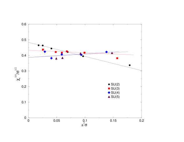
Figure 10: The topological susceptibility in units of the string tension plotted against $a^{2}\sigma$. Continuum extrapolations for each SU($N$) are shown.

In Fig.10 we plot the dimensionless ratio $\chi^{1/4}_{t}/\surd\sigma$ against $a^{2}\sigma$. For sufficiently small $a$ we expect a dependence

$${{\chi^{1\over 4}_{t}(a)}\over{\surd\sigma(a)}}={{\chi^{1\over 4}_{t}(0)}\over{\surd\sigma(0)}}+ca^{2}\sigma.$$ (21)

so that a continuum extrapolation should be a simple stright line on our plot. We show typical best fits of this kind.

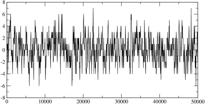
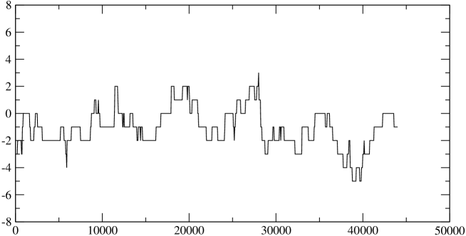
Figure 11: Two sequences of topological charge calculations, made every 50 sweeps, against the number of sweeps. Top is in SU(3) taken on a $16^{4}$ lattice at $\beta=6.0$. Bottom is in SU(5) taken on a $16^{4}$ lattice at $\beta=17.45$.

We see from Fig.10 that the SU(2) and SU(3) calculations are very precise and under good control. As we increase $N$ the errors on the values corresponding to smaller values of $a$ become much larger, and the increasing scatter of points suggests that these error estimates are becoming seriously underestimated. This is to be expected. The Monte Carlo changes $Q$ by an instanton shrinking through small values of $\rho$ down to $\rho\sim a$ where it can vanish through the lattice. (Or the reverse process.) However eqn(18) tells us that the probability of a very small instanton goes rapidly to zero as $N$ grows. Thus the lattice fields rapidly become constrained to lie in given topological sectors and for this quantity the Monte Carlo rapidly ceases to be ergodic as $N$ grows. This is illustrated in Fig.11. Here we show how the value of $Q$ varies in two long Monte Carlo sequences, the first in SU(3) and the second in SU(5). The lattice sizes are the same as is the lattice spacing (within errors) when expressed in units of the string tension. Thus the sequences can be directly compared and it is apparent that the value of $Q$ changes much less frequently in SU(5) than in SU(3).

In Table 11 we list the continuum limit of $\chi^{1/4}_{t}/\surd\sigma$ for each of our SU($N$) groups. In Fig.12 we plot these values against $1/N^{2}$. This is the expected leading large-$N$ correction, so an extrapolation to $N=\infty$ would be a straight line on this plot

$$\left.{{\chi^{1\over 4}_{t}}\over{\surd\sigma}}\right|_{N}=\left.{{\chi^{1\over 4}_{t}}\over{\surd\sigma}}\right|_{\infty}+{c\over N^{2}}.$$ (22)

We show our best such fit in the plot:

$${{\chi^{1\over 4}_{t}}\over{\surd\sigma}}=0.376(20)+{{0.43(10)}\over N^{2}}.$$ (23)

We see from this that the large-$N$ corrections to the SU(3) susceptibility are indeed modest. That is to say, if we express $\lim_{N\to\infty}{\chi_{t}}$ in physical units using $\surd\sigma\sim 440\pm 38MeV$ [35] we obtain the value $(165\pm 17MeV)^{4}$ for the large-$N$ susceptibility – a value that is consistent with our expectations [29] in eqn(15).

6.3 the instanton size distribution

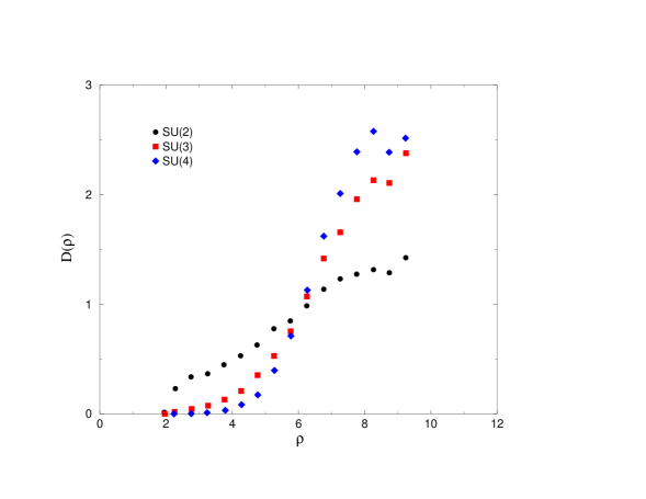
Figure 13: The number density of topological charges plotted as a function of the charge radius, $\rho$; obtained for $N=2,3,4$ from $20^{4}$ lattices with $a\surd\sigma\sim 0.16$.

In Fig.13 we plot the number density of topological charges against their size $\rho$. We do this for the $20^{4}$ SU(2), SU(3) and SU(4) lattices. This is the calculation with the smallest value of $a$ common to these groups. (In fact the value of $a\surd\sigma$ varies a little across these calculations and we have rescaled the number density to take this into account. We have not rescaled the horizontal $\rho$ axis since here the effect is close to negligible.)

We observe that the small-$\rho$ tail disappears rapidly as $N$ increases, just as we expect. This implies, as we have already discussed, that our Monte Carlo must become ineffective in exploring different topological charge sectors as $N$ increases. We observe that the density $D(\rho)$ appears to tend to a large-$N$ limit where there are no charges at all with $\rho\leq\rho_{c}$. In lattice units $\rho_{c}\sim 5-6$ which translates in physical units to $\rho_{c}\sim 0.9/\surd\sigma\sim 0.4fm$. The density then rises rapidly and takes non-zero values over a range of $\rho$. The decrease at small $\rho$ is very roughly consistent with being exponential in $N$, as expected.

As remarked earlier, at small $\rho$ one can make a reliable theoretical prediction for the $\rho$–dependence of $D(\rho)$. To test the prediction in eqn(18), we fit our calculated distributions to the form

$$D(\rho)\propto\rho^{\gamma_{eff}(\rho)}.$$ (24)

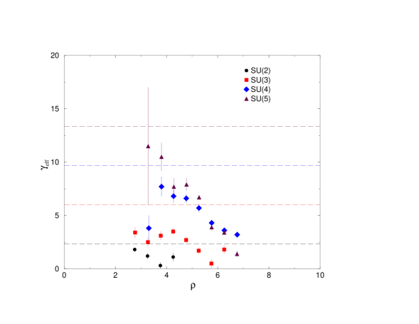
Figure 14: The effective power dependence of the number density of topological charges, $D(\rho)\propto\rho^{\gamma_{eff}}$ compared for $N=2,3,4,5$ on $16^{4}$ lattices with $a\surd\sigma\sim 0.21$. Dashed lines are the theoretical expectations for $\rho\to 0$ taken from eqn(18), with higher lines correspond to larger $N$.

The smallest $a$ common to all our groups is on the $16^{4}$ lattices. We extract $D(\rho)$ and $\gamma_{eff}$ from these calculations and plot the resulting values in Fig.14. We also plot in each case the power, from eqn(18), that we expect to observe for $a\ll\rho\ll 0.5fm$. Values of $\rho$ satisfying these strong inequalities do not exist in our calculation. Nonetheless there is an indication in Fig.14 that our values of $\gamma_{eff}$ are indeed tending to the expected values. This provides evidence that our number densities, while certainly somewhat deformed by the cooling, do retain the main features of the true continuum densities.

7 Conclusions

We have seen, by explicit calculation, that SU($N$) gauge theories in 3+1 dimensions do indeed appear to have a smooth large-$N$ limit that is linearly confining. We find that, as expected, the limit is achieved by keeping the ’t Hooft coupling, $\lambda=g^{2}N$, fixed. Remarkably we found that even SU(2) is close to SU($\infty$) in the sense that a number of basic mass ratios can be described over all $N$ using only a modest $O(1/N^{2})$ correction. Thus a number of simple expressions, such as those in eqns(7–9) and eqn(23), elegantly encapsulate the corresponding physics for all values of $N$. Moreover, this greatly increases the plausibility of arguments that QCD is close to its large-$N$ limit.

The purpose of our calculation was not to obtain the detailed physics of the SU($\infty$) theory, and for that reason we have not attempted to compare our results to the predictions of recent analytic approaches (for example [36] or [37]). Rather our aim has been to establish whether a detailed study is, in practice, possible. Clearly it is, and in Section 4.3 we pointed out some of the lessons we have learned concerning what will be needed to make such a study successful. Nonetheless, our present study has revealed the beginnings of an interesting $N=\infty$ glueball spectrum, with $m_{2^{++}}\simeq 1.5m_{0^{++}}$ and a large excitation gap in the scalar sector, $m_{0^{++\star}}\simeq 2m_{0^{++}}$. However we need a much more detailed spectrum if we are to be able to draw useful dynamical conclusions from it.

We have also seen that the topological susceptibility acquires only small corrections when $N$ is reduced from $N=\infty$ to $N=3$. This provides an a posteriori justification for estimating this suceptibility using the experimental value of $m_{\eta^{\prime}}$.

As described in the Introduction we shall address the interesting physics of the new non-trivial $k$-strings that one encounters for $N\geq 4$ in a parallel publication [7].

SU(2)
$\beta$	lattice	sweeps	$am_{l}$	$a\surd\sigma$	$am_{0^{++}}$	$am_{0^{++\star}}$	$am_{2^{++}}$
2.25	$8^{4}$	$2\times 10^{5}$	1.301(17)	0.4231(25)	1.390(30)	2.5(4)	2.30(25)
2.30	$10^{4}$	$10^{5}$	0.861(11)	0.3108(17)	1.090(33)	1.58(9)	1.64(7)
2.40	$12^{4}$	$10^{5}$	0.745(9)	0.2634(14)	0.953(19)	1.48(5)	1.50(5)
2.475	$16^{4}$	$10^{5}$	0.585(8)	0.2016(13)	0.754(10)	1.19(2)	1.111(19)
2.55	$20^{4}$	$10^{5}$	0.453(4)	0.15896(63)	0.586(10)	0.91(2)	0.874(15)
2.60	$24^{4}$	$10^{5}$	0.387(4)	0.13395(62)	0.514(8)	0.799(10)	0.750(12)

Table 1: The mass of the flux loop, $m_{l}$; the string tension, $\sigma$, as derived from it using eqn(4); the lightest scalar and tensor glueball masses and the first excited scalar mass. For SU(2) on the lattices and at the couplings shown.

SU(3)
$\beta$	lattice	sweeps	$am_{l}$	$a\surd\sigma$	$am_{0^{++}}$	$am_{0^{++\star}}$	$am_{2^{++}}$
5.70	$8^{4}$	$10^{5}$	1.124(15)	0.3961(23)	0.999(25)	2.07(21)	2.03(20)
5.80	$10^{4}$	$10^{5}$	0.886(9)	0.3148(14)	0.895(28)	1.63(10)	1.66(6)
5.90	$10^{4}$	$10^{5}$	0.534(9)	0.2527(18)	0.736(20)	0.95(7)	1.22(4)
5.90	$12^{4}$	$10^{5}$	0.727(9)	0.2605(14)	0.819(19)	1.40(6)	1.30(4)
5.93	$10^{3}16$	$10^{5}$	0.467(7)	0.2391(15)	0.708(22)	1.00(7)	0.94(8)
5.93	$12^{4}$	$10^{5}$	0.6245(62)	0.2435(11)	0.756(20)	1.236(36)	1.21(3)
5.93	$16^{4}$	$10^{5}$	0.879(18)	0.2430(23)	0.780(16)	1.487(43)	1.234(30)
6.00	$16^{4}$	$10^{5}$	0.7071(84)	0.2197(12)	0.734(13)	1.03(8)	1.132(24)
6.20	$20^{4}$	$10^{5}$	0.4603(67)	0.1601(10)	0.544(9)	0.955(20)	0.827(15)

Table 2: The mass of the flux loop, $m_{l}$; the string tension, $\sigma$, as derived from it using eqn(4); the lightest scalar and tensor glueball masses and the first excited scalar mass. For SU(3) on the lattices and at the couplings shown.

SU(4)
$\beta$	lattice	sweeps	$am_{l}$	$a\surd\sigma$	$am_{0^{++}}$	$am_{0^{++\star}}$	$am_{2^{++}}$
10.55	$8^{4}$	$2\times 10^{5}$	0.973(17)	0.3715(28)	0.837(23)	1.76(11)	1.87(10)
10.70	$6^{3}16$	$0.5\times 10^{5}$	0.268(8)	0.2716(14)	0.630(30)	1.44(8)	0.55(5)
10.70	$8^{3}12$	$10^{5}$	0.564(10)	0.2947(21)	0.780(30)	1.22(4)	1.14(6)
10.70	$10^{4}$	$10^{5}$	0.8375(92)	0.3070(15)	0.906(24)	1.74(10)	1.53(7)
10.70	$12^{4}$	$10^{5}$	1.033(11)	0.3055(15)	0.888(30)	1.64(8)	1.54(6)
10.90	$12^{4}$	$10^{5}$	0.621(8)	0.2429(14)	0.720(30)	1.355(40)	1.24(4)
11.10	$16^{4}$	$10^{5}$	0.585(8)	0.2016(13)	0.644(17)	1.183(28)	0.955(55)
11.30	$20^{4}$	$10^{5}$	0.5278(65)	0.1703(10)	0.572(11)	1.125(20)	0.885(15)

Table 3: The mass of the flux loop, $m_{l}$; the string tension, $\sigma$, as derived from it using eqn(4); the lightest scalar and tensor glueball masses and the first excited scalar mass. For SU(4) on the lattices and at the couplings shown.

SU(5)
$\beta$	lattice	sweeps	$am_{l}$	$a\surd\sigma$	$am_{0^{++}}$	$am_{0^{++\star}}$	$am_{2^{++}}$
16.755	$8^{4}$	$10^{5}$	1.051(13)	0.3844(21)	0.777(23)	1.81(17)	2.12(18)
16.975	$10^{4}$	$2\times 10^{5}$	0.816(12)	0.3034(20)	0.874(17)	1.63(6)	1.51(5)
17.27	$12^{4}$	$1.4\times 10^{5}$	0.634(9)	0.2452(15)	0.753(20)	1.39(4)	1.24(4)
17.45	$16^{4}$	$10^{5}$	0.724(12)	0.2221(17)	0.689(15)	1.15(11)	1.110(28)

Table 4: The mass of the flux loop, $m_{l}$; the string tension, $\sigma$, as derived from it using eqn(4); the lightest scalar and tensor glueball masses and the first excited scalar mass. For SU(5) on the lattices and at the couplings shown.

continuum limit
	$m_{0^{++}}/\surd\sigma$	$m_{0^{++\star}}/\surd\sigma$	$m_{2^{++}}/\surd\sigma$
SU(2)	3.844(61)	6.06(16)	5.59(15)
SU(3)	3.607(87)	6.07(30)	5.13(22)
SU(4)	3.49(14)	6.80(45)	5.21(21)
SU(5)	3.38(16)	6.16(55)	4.88(38)
SU($\infty$)	3.37(15)	6.43(50)	4.93(30)

Table 5: The continuum limit of the lightest scalar and tensor glueball masses, and the first excited scalar mass, all in units of the string tension $\sigma$. The extrapolation of these to $N=\infty$ is also shown.

	$\surd\sigma/\Lambda^{eff}_{I}$	range	CL%
SU(2)	5.41(10)	$\beta\geq 2.475$	0.5
SU(3)	5.70(10)	$\beta\geq 5.90$	17
SU(4)	5.89(10)	$\beta\geq 10.70$	90
SU(5)	5.97(8)	$\beta\geq 16.75$	40

Table 6: The continuum limit of the effective perturbative $\Lambda_{I}$ parameter. The range of $\beta$ used and the confidence level of the best fit is shown.

SU(2)
$\beta$	lattice	plaquette	$\langle Q^{2}_{I}\rangle$	$\langle Q^{2}_{Ic}\rangle$	$\langle Q^{2}_{r}\rangle$
2.25	$8^{4}$	0.586207(29)	1.696(43)	0.666(19)	1.397(40)
2.30	$10^{4}$	0.616955(29)	2.268(71)	1.159(46)	1.922(60)
2.40	$12^{4}$	0.629995(17)	3.158(86)	1.664(56)	2.812(86)
2.475	$16^{4}$	0.646921(10)	4.23(15)	2.97(10)	3.84(14)
2.55	$20^{4}$	0.661367(4)	4.73(19)	3.53(12)	4.30(18)
2.60	$24^{4}$	0.670009(3)	5.00(15)	4.22(14)	4.55(14)

Table 7: The fluctuation of the topological charge using three different measures of the charge (see Section 6.1). Also the average plaquette. For SU(2).

SU(3)
$\beta$	lattice	plaquette	$\langle Q^{2}_{I}\rangle$	$\langle Q^{2}_{Ic}\rangle$	$\langle Q^{2}_{r}\rangle$
5.70	$8^{4}$	0.549123(56)	2.151(60)	1.002(38)	1.779(59)
5.80	$10^{4}$	0.567633(12)	2.986(68)	1.767(45)	2.547(63)
5.90	$10^{4}$	0.58187(3)	1.452(62)	1.042(38)	1.205(48)
5.90	$12^{4}$	0.58185(2)	3.147(98)	2.321(75)	2.675(91)
5.93	$10^{3}16$	0.58560(3)	1.830(63)	1.415(53)	1.527(53)
5.93	$12^{4}$	0.585600(15)	2.655(90)	2.066(68)	2.266(78)
5.93	$16^{4}$	0.585580(10)	6.92(25)	5.49(22)	6.47(24)
6.00	$16^{4}$	0.593669(8)	4.83(17)	4.12(14)	4.30(16)
6.20	$20^{4}$	0.613622(7)	3.85(33)	3.72(33)	3.49(31)

Table 8: The fluctuation of the topological charge using three different measures of the charge (see Section 6.1). Also the average plaquette. For SU(3).

SU(4)
$\beta$	lattice	plaquette	$\langle Q^{2}_{I}\rangle$	$\langle Q^{2}_{Ic}\rangle$	$\langle Q^{2}_{r}\rangle$
10.55	$8^{4}$	0.537290(50)	2.48(8)	1.29(5)	2.05(7)
10.70	$8^{3}12$	0.554114(31)	1.477(54)	1.114(35)	1.213(43)
10.70	$10^{4}$	0.554100(20)	2.56(9)	1.99(8)	2.15(8)
10.70	$12^{4}$	0.554105(14)	4.82(16)	3.84(13)	4.25(15)
10.90	$12^{4}$	0.570103(10)	1.97(14)	1.82(12)	1.69(11)
11.10	$16^{4}$	0.583332(5)	2.31(32)	2.26(32)	2.08(29)
11.30	$20^{4}$	0.595014(4)	4.34(76)	4.31(74)	3.98(70)

Table 9: The fluctuation of the topological charge using three different measures of the charge (see Section 6.1). Also the average plaquette. For SU(4).

SU(5)
$\beta$	lattice	plaquette	$\langle Q^{2}_{I}\rangle$	$\langle Q^{2}_{Ic}\rangle$	$\langle Q^{2}_{r}\rangle$
16.755	$8^{4}$	0.52783(5)	2.684(68)	1.674(51)	2.258(67)
16.975	$10^{4}$	0.545164(14)	2.470(75)	2.222(63)	2.083(67)
17.27	$12^{4}$	0.561139(7)	1.65(16)	1.61(16)	1.44(14)
17.45	$16^{4}$	0.569407(5)	3.36(53)	3.35(52)	3.00(47)

Table 10: The fluctuation of the topological charge using three different measures of the charge (see Section 6.1). Also the average plaquette. For SU(5).

$\chi^{1/4}_{t}/\surd\sigma$ : continuum limit
	$Q_{I}$	$Q_{Ic}$	$Q_{r}$
SU(2)	0.4831(56)	0.4745(63)	0.4742(56)
SU(3)	0.434(10)	0.451(8)	0.427(11)
SU(4)	0.387(17)	0.426(15)	0.380(16)
SU(5)	0.387(21)	0.350(30)	0.374(20)

Table 11: The continuum limit of the topological susceptibility $\chi_{t}$ in units of the string tension $\sigma$, for the three different measures of the topological charge indicated.

Figure 2: The mass of the lightest periodic flux loop as a function of its length, at $\beta=10.70$ in SU(4). Shown is a linear fit with a string correction as in eqn(4).

Figure 3: The mass of the lightest periodic flux loop as a function of its length, at $\beta=5.93$ in SU(3). Shown is a linear fit with a string correction as in eqn(4).

Figure 12: The continuum topological susceptibility in units of the string tension plotted against $1/N^{2}$. A linear extrapolation to $N=\infty$ is shown.

References

-
[1]
G. ’t Hooft, Nucl. Phys. B72 (1974) 461.
E. Witten, Nucl. Phys. B160 (1979) 57.
S. Coleman, 1979 Erice Lectures.
A. Manohar, 1997 Les Houches Lectures, hep-ph/9802419. - [2] M. Teper, Phys. Rev. D59 (1999) 014512 (hep-lat/9804008).
- [3] M. Teper, Phys. Lett. B397 (1997) 223 (hep-lat/9701003) and unpublished.
- [4] M. Teper, hep-th/9812187.
- [5] M. Wingate and S. Ohta, hep-lat/0006016; Nucl. Phys. Proc. Suppl. 83 (2000) 381 (hep-lat/9909125).
- [6] B. Lucini and M. Teper, Phys. Lett. B501 (2001) 128 (hep-lat/0012025).
- [7] B. Lucini and M. Teper, in preparation.
-
[8]
A. Hanany, M. J. Strassler and A. Zaffaroni,
Nucl. Phys. B513 (1998) 87 (hep-th/9707244).
M. J. Strassler, Nucl. Phys. Proc. Suppl. 73 (1999) 120 (hep-lat/9810059). - [9] S. Deldar, Phys. Rev. D62 (2000) 034509 (hep-lat/9911008).
- [10] G. Bali, Phys. Rev. D62 (2000) 114503 (hep-lat/0006022).
-
[11]
V. I. Shevchenko and Yu. A. Simonov,
Phys. Rev. Lett. 85 (2000) 1811 (hep-ph/0001299).
Y. Koma, E. -M. Ilgenfritz, H. Toki and T. Suzuki, hep-ph/0103162. - [12] L. Del Debbio, H. Panagopoulos and E. Vicari, in progress.
- [13] N. Cabibbo and E. Marinari, Phys. Lett. B119 (1982) 387.
-
[14]
M. Teper,
Phys. Lett. B183 (1987) 345.
M. Albanese et al (APE Collaboration), Phys. Lett. B192 (1987) 163. - [15] J. Kogut, Rev. Mod. Phys. 55 (1983) 775.
- [16] M. Creutz, Quarks, gluons and lattices (CUP, 1983).
- [17] D. Gross and E. Witten, Phys. Rev. D21 (1980) 446.
- [18] G. Bhanot and M. Creutz, Phys. Rev. D24 (1981) 3212.
-
[19]
R. C. Brower, D. A. Kessler and H. Levine,
Phys. Rev. Lett. 47 (1981) 621.
R. C. Brower, D. A. Kessler, H. Levine, M. Nauenberg and T. Schalk, Phys. Rev. D26 (1982) 959. - [20] I. G. Halliday and A. Schwimmer, Phys. Lett. B101 (1981) 327; B102 (1981) 337. L. Caneschi, I. G. Halliday and A. Schwimmer, Nucl. Phys. B200 (1982) 409; Phys. Lett. B117 (1982) 427.
- [21] M. Lüscher, K. Symanzik and P. Weisz, Nucl. Phys. B173 (1980) 365.
- [22] Ph. de Forcrand, G. Schierholz, H.Schneider and M. Teper, Phys. Lett. B160 (1985) 137.
- [23] K. Ishikawa, G. Schierholz and M. Teper, Z. Phys. C19 (1983) 327.
- [24] C. Morningstar and M. Peardon, Phys. Rev. D56 (1997) 4043 (hep-lat/9704011); Phys. Rev. D60 (1999) 034509 (hep-lat/9901004).
- [25] R. Johnson and M. Teper, Nucl. Phys. Proc. Suppl. 73 (1999) 267 (hep-lat/9808012).
-
[26]
G. Parisi,
in High Energy Physics - 1980 (AIP 1981).
P. Lepage and P. Mackenzie, Phys. Rev. D48 (1993) 2250.
P. Lepage, Schladming Lectures, hep-lat/9607076. -
[27]
M. Luscher, P. Weisz and R. Sommer,
Nucl. Phys. B389 (1993) 247 (hep-lat/9207010).
M. Luscher, Les Houches Lectures, hep-lat/9802029. - [28] G. ’t Hooft, Physics Reports 142 (1986) 357.
-
[29]
E. Witten,
Nucl. Phys. B156 (1979) 269.
G. Veneziano, Nucl. Phys. B159 (1979) 213. - [30] M. Teper, Nucl. Phys. Proc. Suppl. 83 (2000) 146 (hep-lat/9909124).
- [31] E. Witten, Nucl. Phys. B149 (1979) 285.
- [32] M. Teper, Z. Phys. C5 (1980) 233.
- [33] C. Callen, R. Dashen and D. Gross, Phys. Rev. D17 (1978) 2717; D19 (1979) 1826.
- [34] M. Teper, Phys. Lett. 202B (1988) 553.
- [35] M. Teper, Newton Inst. NATO-ASI School Lectures, 1997 (hep-lat/9711011).
- [36] S. Dalley and B. van de Sande, Phys. Rev. D62 (2000) 014507 (hep-lat/9911035).
- [37] O. Aharony, S. S. Gubser, J. Maldacena, H. Ooguri and Y. Oz, Phys. Rept. 323 (2000) 183 (hep-th/9905111).