FERMILAB-PUB-01/035-T HUPD-0104 RCNP-Th01005 UT-CCP-P-102 hep-lat/0103026 $O(a)$-improved quark action on anisotropic lattices and perturbative renormalization of heavy-light currents

Abstract

We investigate the Symanzik improvement of the Wilson quark action on anisotropic lattices. Taking first a general action with nearest-neighbor and clover interactions, we study the mass dependence of the ratio of the hopping parameters, the clover coefficients, and an improvement coefficient for heavy-light vector and axial vector currents. We show how tree-level improvement can be achieved. For a particular choice of the spatial Wilson coupling, the results simplify, and $O(m_{0}a_{\tau})$ improvement is possible. (Here $m_{0}$ is the bare quark mass and $a_{\tau}$ the temporal lattice spacing.) With this choice we calculate the renormalization factors of heavy-light bilinear operators at one-loop order of perturbation theory employing the standard plaquette gauge action.

1 Introduction

The anisotropic lattice has become an important tool in lattice QCD simulations. With a small temporal lattice spacing $a_{\tau}$ one can more easily follow the time evolution of correlators, while keeping the spatial lattice spacing $a_{\sigma}$ comparatively modest [1]. This approach is especially effective when the signal-to-noise ratio deteriorates quickly, as, for example, in the case of glueballs [2]. The better signal-to-noise ratio is beneficial also for heavy quark systems [3]. In addition, it is hoped that the anisotropy can be exploited to reduce lattice artifacts [4], which are a special concern with heavy quarks.

In current work on heavy quarks, lattice artifacts are controlled with non-relativistic QCD (NRQCD) and heavy-quark effective theory (HQET). This is done either a priori, by discretizing the NRQCD action [5], or a posteriori, by using the effective theories to describe lattice gauge theory with Wilson fermions [6, 7]. These strategies are possible because the typical spatial momenta in heavy quark systems are much smaller than the heavy quark mass. Heavy quarkonia have momenta $\mbox{\boldmath$p$}\sim m_{Q}v$ and $k\sim m_{Q}v^{2}$, where $v\sim 0.1$–0.3 is the heavy-quark velocity; heavy-light hadrons have momenta only of order $\Lambda_{\rm QCD}$. In these approaches one is left with discretization effects of order $(\Lambda_{\rm QCD}a)^{n}$ from the light quarks and gluons and of order $\alpha_{s}^{l}(\mbox{\boldmath$p$}/m_{Q})^{n}$ from the heavy quark.

The method of Ref. [6] smoothly connects to the usual continuum limit, so one can, in principle, reduce discretization effects to scale as a power of the lattice spacing $a$, but only by making $a$ too small to be practical. Klassen proposed using anisotropic lattices with the anisotropy $\xi=a_{\sigma}/a_{\tau}$ chosen so that $m_{Q}a_{\tau}$ and $\mbox{\boldmath$p$}a_{\sigma}$ are both small [4]. Clearly, this proposal works only if $p$ is smaller than $m_{Q}$, as in the approaches based explicitly on heavy-quark theory. It also works only if renormalization constants have a smooth limit as $m_{0}a_{\tau}\to 0$, where $m_{0}$ is the bare quark mass. In particular, one would like to be able to expand the renormalization constants in powers of $m_{0}a_{\tau}$ even when $m_{0}a_{\sigma}\sim 1$. Then it may be possible to adjust the improvement parameters of the lattice action (and currents) in a non-perturbative, mass-independent scheme [8, 4]. If, on the other hand, $m_{0}a_{\sigma}$ dependence appears in an essential way, then one would be forced back to a non-relativistic interpretation, as explained for isotropic lattices in Refs. [6, 7].

To our knowledge there is no proof that cutoff effects always appear as powers of $m_{0}a_{\tau}$. In this paper we try to gain some experience by calculating the full mass dependence of several (re)normalization constants, first at tree level and then at one-loop in perturbation theory. We focus on the Fermilab action [6], which is the most general action without doubler states, having different nearest-neighbor and clover couplings in the temporal and spatial directions. This action has been applied on anisotropic lattices to the charmonium system [4, 9, 10, 11, 12], as have some actions with next-to-nearest neighbor interactions. The self-energy has been calculated at the one-loop level in perturbation theory [13].

In the numerical work on charmonium, two different choices for tuning the spatial Wilson term have been made. One choice is that of Refs. [9, 10], where $r_{s}=1/\xi$. Another choice is that of Refs. [4, 11, 12], where $r_{s}=1$. In the first part of this paper, we study improvement conditions for these two choices, as a function of the heavy quark mass. (In a perturbative calculation more generally improved actions with $r_{t}=\xi^{2}\zeta r_{s}$ also have been considered [13].) By studying the full functional dependence on $\xi$ and $m_{0}a_{\tau}$, we can test whether $m_{0}a_{\sigma}$ appears in an essential way. We find that the limit of small $m_{0}a_{\tau}$ is benign at the tree-level only for the first choice, $r_{s}=1/\xi$. For the other choice, $r_{s}=1$, the continuum limit is reached only for $m_{0}a_{\sigma}\ll 1$.

It turns out that with the first choice ($r_{s}=1/\xi$) two of the improvement parameters vanish at the tree-level as $m_{0}a_{\tau}\to 0$. This simplifies the one-loop analysis, so in the second part of the paper we concentrate on this choice. This calculation has two purposes. The first is to study cutoff effects of the renormalization coefficients and to test at the one-loop level whether they still appear only as powers of $m_{0}a_{\tau}$. The second is for phenomenological applications to heavy-light matrix elements. Even if a non-relativistic interpretation is necessary, anisotropic lattices are a good method for reducing the signal-to-noise ratio [3].

This paper is organized as follows. Sec. 2 describes the quark field action and discusses its parametrization in detail. In Sec. 3, the expression for the one-loop perturbative calculation is given. The numerical result for these perturbative constants are presented in Sec. 4. The last section is devoted to our conclusions. We give the Feynman rules in Appendix A and explicit expressions for the one-loop diagrams in Appendix B.

2 Anisotropic quark action

This section describes the actions with Wilson fermions [14] on anisotropic lattices. We denote the renormalized anisotropy with $\xi$, and the spatial and temporal lattice spacings with $a_{\sigma}$ and $a_{\tau}$ respectively:

$$a_{\sigma}=\xi a_{\tau}.$$ (2.1)

These lattice spacings would be defined through the gauge field with quantities such as the Wilson loops or the static quark potential. We therefore consider $\xi$ to be independent of the quark mass.

2.1 Quark field action

Following Ref. [6], let us introduce an action with two hopping parameters [14] and two clover [15] coefficients,

$$S = \sum_{n}\bar{\psi}_{n}\Big{[}\psi_{n}-\kappa_{t}[(r_{t}-\gamma_{4})U_{n,4}\psi_{n+\hat{4}}+(r_{t}+\gamma_{4})U^{\dagger}_{n-\hat{4},4}\psi_{n-\hat{4}}]$$

$$-\kappa_{s}\sum_{i}[(r_{s}-\gamma_{i})U_{n,i}\psi_{n+\hat{\imath}}+(r_{s}+\gamma_{i})U^{\dagger}_{n-\hat{\imath},i}\psi_{n-\hat{\imath}}]$$

$$+{\textstyle\frac{i}{2}}r_{s}c_{B}\kappa_{s}\sum_{i,j,k}\epsilon_{ijk}\sigma_{ij}B_{n,k}\psi_{n}+ic_{E}\kappa_{s}\sum_{i}\sigma_{4i}E_{n,i}\psi_{n}\Big{]}.$$

This is the most general nearest-neighbor clover action. Note that the notation is slightly different than in Ref. [6]; $c_{B}$ of Ref. [6] corresponds to $r_{s}c_{B}$ in (2.1).

It is helpful to change to a notation with a quark mass. We rescale field by

$$\psi_{n}=\frac{a_{\sigma}^{3/2}}{\sqrt{2\kappa_{s}}}\psi(x),$$ (2.3)

and introduce the bare mass

$$m_{0}a_{\tau}=\frac{1}{2\kappa_{t}}-[r_{t}+3r_{s}\zeta],$$ (2.4)

with $\zeta=\kappa_{s}/\kappa_{t}$. Then one can rewrite the action as

$$S = a_{\tau}a_{\sigma}^{3}\sum_{x}\bar{\psi}(x)\left[m_{0}+{\textstyle\frac{1}{2}}(r_{t}+\gamma_{4})D_{4}^{-}-{\textstyle\frac{1}{2}}(r_{t}-\gamma_{4})D_{4}^{+}+\xi\zeta\mbox{\boldmath$\gamma$}\!\cdot\!\mbox{\boldmath$D$}-{\textstyle\frac{1}{2}}a_{\tau}\xi^{2}r_{s}\zeta\triangle^{(3)}\right.$$ (2.5)

$$\left.-{\textstyle\frac{i}{2}}a_{\tau}\xi^{2}r_{s}c_{B}\zeta\mbox{\boldmath$\Sigma$}\!\cdot\!\mbox{\boldmath$B$}-{\textstyle\frac{1}{2}}a_{\tau}\xi c_{E}\zeta\mbox{\boldmath$\alpha$}\!\cdot\!\mbox{\boldmath$E$}\right]\psi(x).$$

The covariant difference operators $D_{4}^{\mp}$, $D$ and $\triangle^{(3)}$, and the fields $B$ and $E$ are defined as in Ref. [6], except that the lattice spacing $a$ is replaced by $a_{\tau}$ or $a_{\sigma}$ in the obvious way.

The action $S$ has six parameters $m_{0}$, $r_{t}$, $r_{s}$, $\zeta$, $c_{B}$, and $c_{E}$. Two are redundant and can be chosen to solve the doubling problem [6]. In particular, we choose $r_{t}=1$ to eliminate doubler states. We then rename $r_{s}=r$, but discuss how to adjust it below. The other four parameters are dictated by physics. The bare mass is adjusted to give the desired physical quark mass, and $\zeta$, $c_{B}$, and $c_{E}$ are chosen to improve the action.

Following Ref. [6] we also consider a rotated field

$$\Psi(x)=e^{M_{1}a_{\tau}/2}\left[1+a_{\sigma}d_{1}\mbox{\boldmath$\gamma$}\!\cdot\!\mbox{\boldmath$D$}\right]\psi(x),$$ (2.6)

where $M_{1}$ is the rest mass, defined and given below, and $d_{1}$ is an improvement parameter. This field is convenient for constructing heavy-light bilinears

$$V_{\mu}^{ub} = \bar{\psi}^{u}\gamma_{\mu}\Psi^{b},$$ (2.7)

$$A_{\mu}^{ub} = \bar{\psi}^{u}\gamma_{\mu}\gamma_{5}\Psi^{b},$$ (2.8)

which, at the tree-level, are correctly normalized currents for all $m_{0}a_{\tau}$. Beyond the tree-level one may add dimension-four terms to these currents, and one must multiply with suitable renormalization factors.

The renormalization factors and the improvement parameters $\zeta$, $c_{B}$, $c_{E}$, and $d_{1}$ must, in general, be chosen to be functions of $m_{0}a_{\tau}$ and the anisotropy $\xi$. Below we shall give the full mass dependence to check whether, for small $m_{0}a_{\tau}$, power series such as

$$\zeta(\xi,m_{0}a_{\tau})=\zeta(\xi,0)+m_{0}a_{\tau}\zeta^{\prime}(\xi,0)$$ (2.9)

can be admitted. If $m_{0}a_{\sigma}=\xi m_{0}a_{\tau}$ enters into the full mass-dependent expression, this series would not be accurate when $m_{0}a_{\sigma}\sim 1$. In the past [4] the behavior in (2.9) was implicitly assumed. If the expansions of the form (2.9) do work, then for full $O(a)$ improvement one must adjust $\zeta(\xi,0)$, $\zeta^{\prime}(\xi,0)$, $c_{B}(\xi,0)$, and $c_{E}(\xi,0)$ in the action, and $Z_{J_{\Gamma}}(\xi,0)$, $Z^{\prime}_{J_{\Gamma}}(\xi,0)$, and $d_{1}(\xi,0)$ of the currents $J_{\Gamma}=V_{\mu}$, $A_{\mu}$.

From (2.5) one can see that conditions for the improvement coefficients can be obtained by simply replacing

$$\zeta \rightarrow \xi\zeta,$$ (2.10)

$$r_{s} \rightarrow \xi r,$$ (2.11)

$$c_{B} \rightarrow \xi rc_{B},$$ (2.12)

$$c_{E} \rightarrow c_{E},$$ (2.13)

in formulae in Ref. [6]. For example, the energy of a quark with momentum $p$ is given by

$$\cosh Ea_{\tau}=1+\frac{(m_{0}a_{\tau}+{\textstyle\frac{1}{2}}\xi^{2}r\zeta\hat{\mbox{\boldmath$p$}}^{2}a_{\tau}^{2})^{2}+\xi^{2}\zeta^{2}\mbox{\boldmath$S$}^{2}a_{\tau}^{2}}{2(1+m_{0}a_{\tau}+{\textstyle\frac{1}{2}}\xi^{2}r\zeta\hat{\mbox{\boldmath$p$}}^{2}a_{\tau}^{2})},$$ (2.14)

where $\hat{p}_{i}=2a_{\sigma}^{-1}\sin({\textstyle\frac{1}{2}}p_{i}a_{\sigma})$ and $S_{i}=a_{\sigma}^{-1}\sin(p_{i}a_{\sigma})$. For small momentum $E^{2}=M_{1}^{2}+\mbox{\boldmath$p$}^{2}M_{1}/M_{2}+O(\mbox{\boldmath$p$}^{4}a^{2})$, where the rest mass $M_{1}$ and kinetic mass $M_{2}$ are

$$M_{1}a_{\tau} = \ln(1+m_{0}a_{\tau}),$$ (2.15)

$$\frac{1}{M_{2}a_{\tau}} = \xi^{2}\left(\frac{2\zeta^{2}}{m_{0}a_{\tau}(2+m_{0}a_{\tau})}+\frac{r\zeta}{1+m_{0}a_{\tau}}\right).$$ (2.16)

To obtain a relativistic quark one sets the rest mass and kinetic mass equal to each other. This yields the condition

$$\xi\zeta=\sqrt{\left(\frac{\xi rm_{0}a_{\tau}(2+m_{0}a_{\tau})}{4(1+m_{0}a_{\tau})}\right)^{2}+\frac{m_{0}a_{\tau}(2+m_{0}a_{\tau})}{2\ln(1+m_{0}a_{\tau})}}-\frac{\xi rm_{0}a_{\tau}(2+m_{0}a_{\tau})}{4(1+m_{0}a_{\tau})},$$ (2.17)

which can be read off from Ref. [6]. Matching of on-shell three-point functions yields the conditions

$$c_{B} = 1,$$ (2.18)

$$c_{E} = \frac{(\xi\zeta)^{2}-1}{m_{0}a_{\tau}(2+m_{0}a_{\tau})}+\frac{\xi^{2}r\zeta}{1+m_{0}a_{\tau}}+\frac{\xi^{2}r^{2}m_{0}a_{\tau}(2+m_{0}a_{\tau})}{4(1+m_{0}a_{\tau})^{2}}$$ (2.19)

on the clover coefficients, and

$$d_{1} = \frac{\xi\zeta(1+m_{0}a_{\tau})}{m_{0}a_{\tau}(2+m_{0}a_{\tau})}-\frac{1}{2M_{2}a_{\tau}}$$ (2.20)

$$= \frac{\xi\zeta[2(1+m_{0}a_{\tau})^{2}-\xi rm_{0}a_{\tau}(2+m_{0}a_{\tau})-2\xi\zeta(1+m_{0}a_{\tau})]}{2m_{0}a_{\tau}(2+m_{0}a_{\tau})(1+m_{0}a_{\tau})}$$ (2.21)

on the rotation parameter. These tree-level formulae (2.14)–(2.21) have been obtained independently by M. Okamoto [16]. We see that essential dependence on $m_{0}a_{\sigma}=\xi m_{0}a_{\tau}$ indeed may arise, depending on how $r$ is tuned.

From the energy (2.14) one can also find the energy of states at the edge of the Brillouin zone. The energy of a state with $n$ components of $p$ equal to $\pi/a_{\sigma}$ is

$$E_{n}a_{\tau}=\ln(1+m_{0}a_{\tau}+2nr\zeta).$$ (2.22)

Although there is some freedom to choose $r$, discussed below, one still wants to keep $E_{n}$ and $M_{1}$ well separated.

For small $m_{0}a_{\tau}$ the interesting Taylor expansions are

$$\zeta = \xi^{-1}+{\textstyle\frac{1}{2}}(\xi^{-1}-r)m_{0}a_{\tau}+O((m_{0}a_{\tau})^{2}),$$ (2.23)

$$c_{E} = {\textstyle\frac{1}{2}}(1+\xi r)+O(m_{0}a_{\tau}),$$ (2.24)

$$d_{1} = {\textstyle\frac{1}{4}}(1-\xi r)+O(m_{0}a_{\tau}).$$ (2.25)

With the mass dependent factor in (2.6) there is no mass dependence at the tree-level in the currents’ normalization factors.

Let us now discuss the choice of the redundant coefficient of the spatial Wilson term $r$. Two choices have been used in numerical calculations:

1. $r=1/\xi$  [9, 10]. This is a natural choice because then the mass form of the action takes a symmetric-looking form, without $\xi$. In the small $m_{0}a_{\tau}$ limit, the tree-level improvement parameters become

   $$\zeta(\xi,0) = \xi^{-1}$$ (2.26)

   $$\zeta^{\prime}(\xi,0) = 0$$ (2.27)

   $$c_{B}(\xi,0) = 1$$ (2.28)

   $$c_{E}(\xi,0) = 1$$ (2.29)

   $$d_{1}(\xi,0) = 0$$ (2.30)

   A key advantage is that $m_{0}a_{\sigma}$ does not appear; the continuum limit is reached for small $m_{0}a_{\tau}$. Furthermore, both $\zeta^{\prime}(\xi,0)$ and $d_{1}(\xi,0)$ vanish at the tree-level, which is especially helpful in one-loop calculations. A disadvantage is that with $r=\zeta=1/\xi$ the energy splitting between physical states and states at the edge of the Brillouin zone is not large. One can circumvent this problem to some extent by choosing appropriate cutoffs and anisotropy [10].

2. $r=1$  [4, 11, 12]. Now all hopping terms in (2.1) have projection matrices ${\textstyle\frac{1}{2}}(1\mp\gamma_{\mu})$, and the anisotropic nature appears only in $\zeta$ and $c_{B}\neq c_{E}$. But now, if one considers what happens to the conditions when $m_{0}a_{\sigma}\mathrel{\raise 1.29167pt\hbox{$<$\kern-7.5pt\lower 4.30554pt\hbox{$\sim$}}}1$ while $m_{0}a_{\tau}\ll 1$, then

   $$\xi\zeta(\xi,m_{0}a_{\tau}) = 1-{\textstyle\frac{1}{2}}m_{0}a_{\sigma}+{\textstyle\frac{1}{8}}(m_{0}a_{\sigma})^{2}+{\textstyle\frac{1}{2}}m_{0}a_{\tau}\left[1-{\textstyle\frac{1}{2}}m_{0}a_{\sigma}\right]$$ (2.31)

   $$c_{E}(\xi,m_{0}a_{\tau}) = {\textstyle\frac{1}{2}}\left[1+\xi\left(1+{\textstyle\frac{1}{2}}m_{0}a_{\sigma}+{\textstyle\frac{1}{8}}(m_{0}a_{\sigma})^{2}\right)\right]$$ (2.32)

   $$d_{1}(\xi,m_{0}a_{\tau}) = \frac{(m_{0}a_{\sigma})^{2}}{16m_{0}a_{\tau}}+{\textstyle\frac{1}{4}}(1-\xi)$$ (2.33)

   keeping terms of order $(m_{0}a_{\sigma})^{2}$ and $m_{0}a_{\tau}m_{0}a_{\sigma}$. Clearly, the continuum limit sets in only when $m_{0}a_{\sigma}\ll 1$. Even then $\zeta^{\prime}$ and $d_{1}$ are non-zero already at the tree-level. An advantage is that the splitting between the physical states and the edge of the Brillouin zone is larger than in case (i).

   In passing we mention that Refs. [4, 11, 12] take

   $$\zeta=\frac{1}{\xi}\frac{2+m_{0}a_{\tau}}{2+\xi m_{0}a_{\tau}}$$ (2.34)

   which agrees with the Taylor expansion (2.23), but does not agree with the full mass dependence (2.17). The denominator of this expression also is of the form that reaches the continuum limit only when $m_{0}a_{\sigma}\ll 1$.

It is instructive to examine the difference between the two conditions on $\zeta^{\prime}$ by considering the full mass dependence of $\zeta$. Figure 1 plots the right-hand side of (2.17)

Figure 1: The tree-level relation of $\zeta$ with the quark mass in the spatial lattice unit, $m_{0\sigma}$, for various $\xi$. The solid and the dotted lines are for choices (i) and (ii) respectively.

against $m_{0\sigma}:=m_{0}a_{\sigma}$, for several values of $\xi$ and the two choices $r=1/\xi$ and $r=1$. The mass in spatial lattice units, $m_{0\sigma}$ is chosen not because it is a natural variable, but because one usually would first fix the spatial lattice spacing $a_{\sigma}$ so that $\mbox{\boldmath$p$}a_{\sigma}$ is small enough, while $m_{0}a_{\sigma}\sim 1$. One would then choose the anisotropy $\xi$ to make $m_{0}a_{\tau}$ small. For example, let us consider the charmed quark on a lattice with $a_{\sigma}^{-1}=1$ GeV. The quark mass in spatial lattice units is $m_{0\sigma}\simeq 1.2$, so if $\xi=4$, then $m_{0}a_{\tau}\simeq 0.3$, which seems small. For $r=1/\xi$ one finds $\zeta(\xi,m_{0}a_{\tau})=\zeta(4,0.3)\approx 0.26$, which is only 4 percent larger than $\zeta(4,0)=0.25$. In this sense, $m_{0}a_{\tau}\simeq 0.3$ is small. On the other hand, for the choice $r=1$, $\zeta(\xi,m_{0}a_{\tau})=\zeta(4,0.3)\approx 0.20$, which is 20 percent smaller than $\zeta(4,0)$. Even worse, the Taylor expansion (2.23) estimates only 0.14.

Thus, only with the choice $r=1/\xi$ does it seem possible to approximate the improvement coefficients by the small $m_{0}a_{\tau}$ limit. With this choice it seems possible to treat charmed quarks, without appealing to the heavy-quark expansion, at accessible spatial lattice spacings and anisotropy around 3–4. Lattice artifacts appear under control and there is probably enough room between $M_{1}$ and the energies at the edge of the Brillouin zone, $E_{n}$, to accommodate the lowest excitations of the $D$ meson. On the other hand, it seems that reasonable choices of $a_{\sigma}$ and $\xi$ do not exist for treating the $b$ quark: $m_{b}a_{\tau}$ remains big, requiring a non-relativistic interpretation along the lines of Refs. [6, 7].

The choice $r=1/\xi$ requires no tree-level rotation for the quark field. This is a great simplification for one-loop renormalization. Then the quark and anti-quark field operators are multiplied by the factor $\exp(M_{1}a_{\tau}/2)=1+{\textstyle\frac{1}{2}}M_{1}a_{\tau}+O((M_{1}a_{\tau})^{2})$. With the choice $r=1$ one would have to include the rotation term for a consistent $O(a_{\tau})$ calculation. In the rest of this paper, we therefore focus on $r=1/\xi$.

3 One-loop Renormalization

To carry out one-loop perturbative calculations, we must specify the gauge field action as well as the quark action. We begin this section with the gauge field action and remark on the gauge couplings, which, in general, differ for the spatial and temporal components of the gauge field. Feynman rules required at one-loop level are summarized in Appendix A.

The self-energy at the one-loop level is represented by the diagrams in Fig. 2(a)–(b).

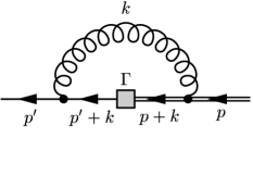
(a)                                      (b)                                      (c)

Figure 2: Feynman diagrams for the quark self-energy (a) and (b), and for the vertex correction (c).

We calculate, as a function of $m_{0}a_{\tau}$, the one-loop contribution to the quark rest mass and wave function renormalization factor. These quantities require the self-energy and its first derivative with respect to the external momentum $p_{4}$, evaluated on the mass shell $(p_{4},\mbox{\boldmath$p$})=(iM_{1},\mbox{\bf 0})$ [17]. By obtaining the full mass dependence, we can check how the one-loop corrections behave for $m_{0}a_{\sigma}\sim 1$ and $m_{0}a_{\tau}$ small. We also discuss mean field improvement of the self-energy. In the past, the full mass dependence of the one-loop quark self-energy has been obtained for the Wilson action on isotropic lattices [18] for the Fermilab action on isotropic lattices [17], and for several improved actions with $r_{t}=\xi^{2}\zeta r_{s}$ on anisotropic lattices [13].

We also discuss vertex corrections at the one-loop level, shown in Fig. 2(c), and present matching factors for the vector and axial vector currents. We again obtain the full mass dependence first, and use it to study the practical situation with $m_{0}a_{\sigma}\sim 1$ and $m_{0}a_{\tau}$ small. In the past, the full mass dependence of the one-loop quark vertex functions has been obtained on isotropic lattices for the Wilson action [18], the clover action [19], and the Fermilab action [20].

3.1 Gauge field action

We use the standard Wilson gauge action on the anisotropic lattice [1]:

$$S_{\rm gauge}=\beta a_{\tau}a_{\sigma}^{3}\sum_{x}\left[\sum_{i<j=1}^{3}\frac{1}{\gamma_{G}}\left(1-{\textstyle\frac{1}{3}}\mathop{\rm Re}\mathop{\rm tr}U_{ij}(x)\right)+\sum_{i=1}^{3}\gamma_{G}\left(1-{\textstyle\frac{1}{3}}\mathop{\rm Re}\mathop{\rm tr}U_{i4}(x)\right)\right],$$ (3.1)

where $U_{\mu\nu}$ denotes parallel transport around a plaquette in the $\mu\nu$ plane. The bare anisotropy $\gamma_{G}$ coincides with the renormalized isotropy $\xi$ at the tree-level. In gauge field theory with $N_{c}$ colors, the coupling $\beta$ is related to the usual bare gauge coupling $g_{0}$ by $\beta=2N_{c}/g_{0}^{2}$.

There is a subtlety in the gauge coupling, because the temporal and spatial gluons have different couplings [1]. One can rewrite $\beta$ and $\gamma_{G}$ as

$$\beta_{\sigma} = \frac{2N_{c}}{g^{2}_{\sigma}(a_{\sigma},\xi)}=\frac{\beta}{\gamma_{G}},$$ (3.2)

$$\beta_{\tau} = \frac{2N_{c}}{g^{2}_{\tau}(a_{\sigma},\xi)}=\beta\gamma_{G},$$ (3.3)

where $g_{\sigma}^{2}$ and $g_{\tau}^{2}$ are couplings for spatial and temporal gluons, respectively. Although at the one-loop level $g_{\sigma}^{2}$ and $g_{\tau}^{2}$ need not be distinguished, it is convenient to separate the results for spatial and temporal parts. To improve perturbative series, it is crucial to use renormalized couplings, defined at the momentum scale typical for the process under consideration [22]. These couplings, and therefore the scales, could be defined separately for spatial and temporal gluons. With this end in mind, we shall present the coefficients of $g_{\sigma}^{2}$ and $g_{\tau}^{2}$ separately.

3.2 Rest mass renormalization

The relation between the rest mass to the self-energy is [17]

$$e^{M_{1}a_{\tau}}=1+m_{0}a_{\tau}-\mathop{\rm tr}[P_{+}\Sigma(iM_{1},\mbox{\bf 0})]a_{\tau},$$ (3.4)

where $P_{+}=(1+\gamma_{4})/2$ and the self-energy $\Sigma(p_{4},\mbox{\boldmath$p$})$ is the sum of all one-particle irreducible two-point diagrams. The formula (3.4) is valid for all masses and at every order in perturbation theory. Since it is obtained from the pole position, the rest mass is infrared finite and gauge independent at every order in perturbation theory [21]. We write the perturbation series as

$$\Sigma(ip_{4},\mbox{\boldmath$p$})=\sum_{l=1}^{\infty}g^{2l}\Sigma^{[l]}(p_{4},\mbox{\boldmath$p$};m_{0}),$$ (3.5)

where we explicitly specify the bare quark mass $m_{0}$. The quark is massless ($M_{1}=0$) when the bare mass is tuned to

$$m_{0c}=\mathop{\rm tr}[P_{+}\Sigma(0,\mbox{\bf 0};m_{0c})].$$ (3.6)

It is more convenient to introduce a subtracted bare mass $M_{0}=m_{0}-m_{0c}$, which vanishes for a massless quark. Then the formula for the rest mass becomes

$$e^{M_{1}a_{\tau}}=1+M_{0}a_{\tau}-\mathop{\rm tr}[P_{+}\bar{\Sigma}(iM_{1},\mbox{\bf 0};M_{0})]a_{\tau},$$ (3.7)

where

$$\bar{\Sigma}(p_{4},\mbox{\boldmath$p$};M_{0})]=\Sigma(p_{4},\mbox{\boldmath$p$};m_{0})-m_{0c}.$$ (3.8)

In developing the perturbation series, now $M_{0}$ is treated independently from $g^{2}$.

The perturbative series for $M_{1}$ is

$$M_{1}=M_{1}^{[0]}+\sum_{l=1}^{\infty}g^{2l}M_{1}^{[l]}.$$ (3.9)

From (3.7)

$$M_{1}^{[0]} = a_{\tau}^{-1}\ln(1+M_{0}a_{\tau}),$$ (3.10)

$$M_{1}^{[1]} = -\frac{\mathop{\rm tr}[P_{+}\bar{\Sigma}^{[1]}(iM_{1},\mbox{\bf 0};M_{0})]}{1+M_{0}a_{\tau}}.$$ (3.11)

In evaluating $\Sigma^{[1]}$ one may disregard the distinction between $M_{0}$ and $m_{0}$, because $m_{0c}$ starts at one-loop order. To show the mass dependence it is convenient [17] to introduce the multiplicative renormalization factor $Z_{M_{1}}$ defined by,

$$M_{1}a_{\tau}=Z_{M_{1}}\tanh M_{1}^{[0]}a_{\tau}.$$ (3.12)

From $Z_{M_{1}}^{[1]}=M_{1}^{[1]}a_{\tau}/\tanh M_{1}^{[0]}a_{\tau}$ one can then remove the anomalous dimension by writing

$$Z_{M_{1}}^{[1]}=C_{F}\left[c^{[1]}-\frac{3}{16\pi^{2}}\ln(M_{1}^{2}a_{\tau}^{2})\right].$$ (3.13)

Numerical results for $M_{1}^{[1]}a_{\tau}$ and $c^{[1]}$ are given in Sec. 4.

3.3 Wave function renormalization

The all orders formula for the wave function renormalization factor is [17]

$$Z_{2}^{-1}=e^{M_{1}a_{\tau}}-\mathop{\rm tr}[P_{+}\dot{\Sigma}(iM_{1},\mbox{\bf 0};M_{0})]a_{\tau}$$ (3.14)

where

$$\dot{\Sigma}(p_{4},\mbox{\boldmath$p$};M_{0})=\frac{1}{i}\frac{\partial\bar{\Sigma}}{\partial p_{4}}(p_{4},\mbox{\boldmath$p$};M_{0}).$$ (3.15)

In view of the mass dependence, we write

$$(1+M_{0}a_{\tau})Z_{2}=1+\sum_{l=1}^{\infty}g^{2l}Z_{2}^{[l]},$$ (3.16)

so that the $Z_{2}^{[l]}$ are only mildly mass dependent. This definition of $Z_{2}^{[l]}$ is slightly different from that of Ref. [17] for $l>1$.

The wave function renormalization factor is infrared divergent and gauge dependent. Therefore we express the one-loop term as

$$Z_{2}^{[1]} = (1+M_{0}a_{\tau})^{-1}\mathop{\rm tr}[P_{+}(\bar{\Sigma}^{[1]}+\dot{\Sigma}^{[1]})],$$ (3.17)

$$=: W^{[1]}+L^{[1]},$$ (3.18)

where $W^{[1]}$ and $L^{[1]}$ are the infrared finite and singular parts, respectively. The infrared divergence does not depend on the ultraviolet regulator, so it is the same as in the continuum theory. We define $L^{[1]}$ by the continuum expression. For a massive quark ($\lambda^{2}\ll m^{2}\ll a_{\tau}^{-2}$) in Feynman gauge,

$$L_{h}^{[1]}=\frac{C_{F}}{16\pi^{2}}\left[-\frac{9}{2}+3\ln(m^{2}a_{\tau}^{2})-2\ln(\lambda^{2}a_{\tau}^{2})\right],$$ (3.19)

which we use for the heavy quark. In particular, $W_{h}^{[1]}$ is defined by combining (3.18) and (3.19) with $m=M_{2}^{[0]}$. For a massless quark ($m^{2}=0$, $\lambda^{2}\ll a_{\tau}^{-2}$), the mass singularity seen in (3.19) can still be regulated by the gluon mass. In Feynman gauge,

$$L_{l}^{[1]}=\frac{C_{F}}{16\pi^{2}}\ln(a_{\tau}^{2}\lambda^{2}),$$ (3.20)

which we use for the light quark. Here $C_{F}=N_{c}^{2}-1/2N_{c}$ [$=4/3$ for SU(3)]. Because the infrared and mass singularities have been subtracted consistently, we should (and do) find $\lim_{m_{0}\to 0}W_{h}^{[1]}=W_{l}^{[1]}$. Numerical results for $W_{h}^{[1]}$ and $W_{l}^{[1]}$ are in Sec. 4.

3.4 Mean field improvement

Mean field improvement [22] has been employed extensively in Monte Carlo work to improve tree-level estimates of couplings. The approximation works, because most of the one-loop coefficients can be traced, via tadpole diagrams, to a mean field. On the anisotropic lattice, the mean field values of the link variables can be defined individually for the temporal and the spatial links. We denote them by $u_{\tau}$ and $u_{\sigma}$ respectively. Then mean field improvement is achieved by replacing the link variables with [4, 9, 10, 11, 12]

$$U_{4}\rightarrow U_{4}/u_{\tau},\hskip 28.45274ptU_{j}\rightarrow U_{j}/u_{\sigma}\hskip 14.22636pt\mbox{($j=\mbox{1--3}$)}.$$ (3.21)

With mean field improvement, the one-loop counter-terms of $u_{\tau}$ and $u_{\sigma}$ must be removed from perturbative coefficients.

Here we consider generically the $O(g^{2})$ contributions from the mean field to the self-energy. From the Feynman rules in Appendix A, the self-energy and its first derivative with respect to $p_{4}$, on the mass shell $({p_{4}},\mbox{\boldmath$p$})=(iM_{1},\mbox{\bf 0})$, are

$$\Sigma_{\rm MF}^{[1]}(iM_{1},\mbox{\bf 0}) = -g^{2}u^{[1]}_{\sigma}3r\zeta-g^{2}u^{[1]}_{\tau}e^{M_{1}^{[1]}a_{\tau}}$$ (3.22)

$$\bar{\Sigma}_{\rm MF}^{[1]}(iM_{1},\mbox{\bf 0}) = -g^{2}u^{[1]}_{\tau}M_{0}a_{\tau}$$ (3.23)

$$\dot{\Sigma}_{\rm MF}^{[1]}(iM_{1},\mbox{\bf 0}) = +g^{2}u^{[1]}_{\tau}e^{M_{1}^{[1]}a_{\tau}}$$ (3.24)

Then, the mean field contribution to the rest mass is

$$M_{1\rm(MF)}^{[1]}a_{\tau}=\frac{M_{0}a_{\tau}}{1+M_{0}a_{\tau}}u^{[1]}_{\tau},$$ (3.25)

and to the wave function renormalization factor

$$W_{\rm MF}^{[1]}=\frac{1}{1+M_{0}a_{\tau}}u^{[1]}_{\tau},$$ (3.26)

which holds for massive and massless ($M_{0}=0$) quarks. The explicit values of $u_{\sigma}^{[1]}$ and $u_{\tau}^{[1]}$ depend on the definition of the mean field. Since one can easily incorporate the contributions from the mean field improvement to the one-loop coefficients, we do not employ a specific scheme and quote only the contributions from the loop integrations.

3.5 Quark bilinear operators

To obtain improved matrix elements, operators also must be improved [23]. As discussed in Sec. 2, with the choice $r=1/\xi$ only the multiplicative factor $\exp(M_{1}a_{\tau}/2)=1+\frac{1}{2}M_{1}a_{\tau}+O(a_{\tau}^{2})$ is required at the tree-level. In particular, with $r=1/\xi$ no new dimension-four operator is needed to achieve tree-level improvement. At higher loop order the counterpart of the mass-dependent factor comes from the quark self-energy through the wave function factor, as seen in (3.14), and dimension-four terms are needed.

Because the tree-level rotation coefficient $d_{1}$ vanishes as $m_{0}a_{\tau}\to 0$, we consider here currents of the form

$$J_{\Gamma}(x)=\bar{\psi}_{l}\Gamma\psi_{h}(x),$$ (3.27)

where $\psi_{l}$ and $\psi_{h}$ are the light and heavy quark fields respectively. We consider the vector and axial vector currents, so the the $4\times 4$ matrix $\Gamma$ is one of $\gamma_{4}$ ($V_{4}$), $\gamma_{j}$ ($V_{j}$), $\gamma_{5}\gamma_{4}$ ($A_{4}$), and $\gamma_{5}\gamma_{j}$ ($A_{j}$). We seek the matching factors $Z_{J_{\Gamma}}$ such that $Z_{J_{\Gamma}}J_{\Gamma}$ has the same matrix elements (for $\mbox{\boldmath$p$}a_{\sigma}\ll 1$) as the continuum bilinear. These matching factors are composed of two parts: the wave function of each quark field and the correction to the vertex. Since the former is already obtained in previous subsection, here we discuss the vertex corrections.

The vertex function $\Lambda_{\Gamma}$, which is the sum of one-particle irreducible three-point diagrams, can be expanded

$$\Lambda_{\Gamma}=1+\sum_{l=1}^{\infty}g^{2l}\Lambda_{\Gamma}^{[l]}.$$ (3.28)

As with the wave function renormalization, $\Lambda_{\Gamma}$ is gauge dependent and suffers from infrared and mass singularities. For the one-loop term we again subtract of the divergent part,

$$\Lambda_{\Gamma}^{[1]}=V_{\Gamma}^{[1]}+L_{\Gamma}^{[1]},$$ (3.29)

where, in Feynman gauge,

$$L_{\Gamma}^{[1]}=\frac{C_{F}}{16\pi^{2}}\left(-{\textstyle\frac{1}{2}}(HG-1)-\ln(\lambda^{2}a_{\tau}^{2})\right).$$ (3.30)

The constants are again taken from the continuum expression, so $HG=-2$ for temporal components of the currents and $HG=2$ for spatial components.

The sought-after matching factor $Z_{J_{\Gamma}}$ is simply the ratio of the lattice and continuum radiative corrections:

$$Z_{J_{\Gamma}}=\frac{\left[Z_{2h}^{1/2}\Lambda_{\Gamma}Z_{2l}^{1/2}\right]^{\rm cont}}{\left[Z_{2h}^{1/2}\Lambda_{\Gamma}Z_{2l}^{1/2}\right]^{\rm lat}}.$$ (3.31)

In view of the mass dependence, we write

$$(1+M_{0}a_{\tau})^{1/2}Z_{J_{\Gamma}}=1+\sum_{l=1}^{\infty}g^{2l}Z_{J_{\Gamma}}^{[l]},$$ (3.32)

so that the $Z_{J_{\Gamma}}^{[l]}$ are only mildly mass dependent. At the one-loop level we have consistently defined the finite lattice parts so that

$$Z_{J_{\Gamma}}^{[1]}=-\left({\textstyle\frac{1}{2}}W_{h}^{[1]}+V_{\Gamma}^{[1]}+{\textstyle\frac{1}{2}}W_{l}^{[1]}\right)$$ (3.33)

is the desired one-loop coefficient of the matching factor. It is gauge invariant and independent of the scheme for regulating the infrared and (light-quark) mass singularities. Numerical results for $V_{\Gamma}^{[1]}$ and $Z_{J_{\Gamma}}^{[1]}$ are in Sec. 4.

4 Numerical results of one-loop perturbation theory

In this section we present our results for the one-loop coefficients. They are obtained numerically using the Monte Carlo integration program BASES [24]. We give one-loop terms for the rest mass, i.e., $M_{1}^{[1]}$ and $c^{[1]}$; for the infrared-finite parts of the wave function renormalization factors and the vertex functions, i.e., $W_{l}^{[1]}$, $W_{h}^{[1]}$ and $V_{\Gamma}^{[1]}$; and for the currents’ matching factors $Z_{J_{\Gamma}}^{[1]}$. In this section we are concerned with zero three-momentum, so for brevity we set the temporal lattice spacing $a_{\tau}=1$. When the spatial lattice spacing is needed, we use the anisotropy $\xi$.

The spatial and the temporal parts of $M_{1}^{[1]}$ are listed separately, namely

$$g^{2}M_{1}^{[1]}\to g^{2}_{\tau}M^{[1]}_{1\tau}+g^{2}_{\sigma}M^{[1]}_{1\sigma},$$ (4.1)

so that one could use different (improved) couplings in a practical evaluation of the perturbative rest mass. On the other hand, for the other quantities we show the combined values of the spatial and the temporal parts, because we are interested mostly in seeing how they behave when $M_{0}\xi\sim 1$ while $M_{0}:=M_{0}a_{\tau}$ small.

The spatial and the temporal parts of $M_{1}^{[1]}$, $M_{1\sigma}^{[1]}$ and $M_{1\tau}^{[1]}$ respectively, are listed in Table 1 for a range of $M_{0}<1$ at four values of $\xi$: 1, 2, 3 and 4.

Table 1: The one-loop correction to the rest mass, $M_{1}^{[0]}$, for various values of $M_{0}$ at four values of $\xi$.

	$M_{0}$	$\xi=1$	$\xi=2$	$\xi=3$	$\xi=4$
$M_{1\sigma}^{[1]}$	0.01	0.00111(3)	0.00151(1)	0.001477(7)	0.001456(5)
	0.02	0.00286(3)	0.00266(1)	0.002571(7)	0.002534(5)
	0.05	0.00624(3)	0.00543(1)	0.005116(7)	0.004958(5)
	0.10	0.01036(3)	0.00868(1)	0.008017(7)	0.007563(5)
	0.20	0.01620(3)	0.01282(1)	0.011177(7)	0.009938(5)
	0.30	0.02002(3)	0.01504(1)	0.012449(6)	0.010507(4)
	0.50	0.02434(2)	0.01665(1)	0.012582(6)	0.009810(4)
	1.00	0.02694(2)	0.015300(9)	0.009960(4)	0.006959(3)
$M_{1\tau}^{[1]}$	0.01	0.00251(1)	0.002018(5)	0.001895(3)	0.001847(2)
	0.02	0.00469(1)	0.003674(6)	0.003423(3)	0.003333(3)
	0.05	0.01049(2)	0.007864(7)	0.007236(4)	0.006959(3)
	0.10	0.01878(2)	0.013606(7)	0.012275(5)	0.011562(4)
	0.20	0.03222(2)	0.022430(8)	0.019480(5)	0.017757(4)
	0.30	0.04305(2)	0.029095(7)	0.024581(6)	0.021753(5)
	0.50	0.05988(2)	0.038651(9)	0.031177(6)	0.026528(6)
	1.00	0.08646(2)	0.05215(1)	0.039395(7)	0.031916(6)

We plot $c^{[1]}$ vs. $M_{0}$ in Fig. 3, and the numerical values are given in Table 2.

Table 2: The non-logarithmic part of the mass renormalization factor $c^{[1]}$.

	$M_{0}$	$\xi=1$	$\xi=2$	$\xi=3$	$\xi=4$
$c^{[1]}$	0.01	0.143(2)	0.092(1)	0.0798(4)	0.0751(3)
	0.02	0.145(1)	0.092(1)	0.0790(2)	0.0738(2)
	0.05	0.1438(4)	0.0900(2)	0.0760(1)	0.0690(1)
	0.10	0.1408(2)	0.08701(8)	0.07104(6)	0.06181(4)
	0.20	0.1370(1)	0.08197(5)	0.06309(3)	0.05070(2)
	0.30	0.13374(7)	0.07828(4)	0.05744(2)	0.04354(2)
	0.50	0.13004(5)	0.07365(2)	0.05110(1)	0.03662(1)
	1.00	0.12787(3)	0.07043(1)	0.04781(1)	0.03473(1)

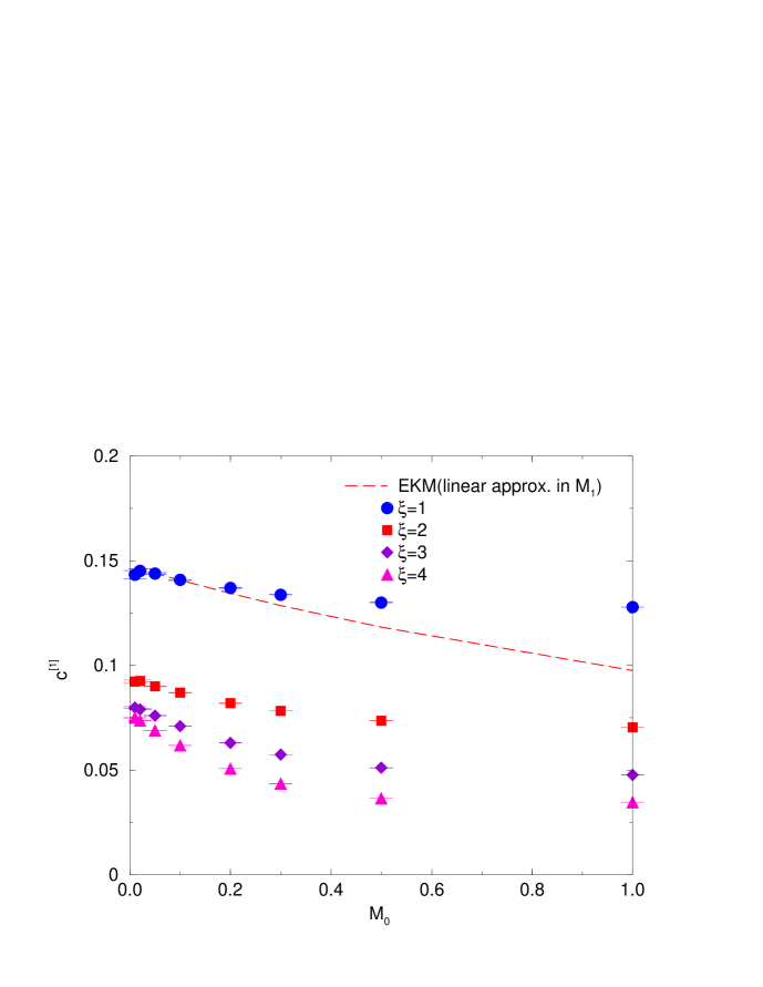
Figure 3: The non-logarithmic part of the mass renormalization factor $c^{[1]}$. The dashed line is the linear approximation, based on Ref. [17].

One sees that the mass dependence is significant, but not drastic.

Table 3 lists the one-loop corrections $W_{l}^{[1]}$

Table 3: The one-loop correction to the light and the heavy quark wave functions.

	$M_{0}$	$\xi=1$	$\xi=2$	$\xi=3$	$\xi=4$
$W_{l}^{[1]}$	0.00	0.08194(2)	0.02994(1)	0.01911(1)	0.01605(1)
$W_{h}^{[1]}$	0.01	0.08009(19)	0.02913(13)	0.01890(11)	0.01621(11)
	0.02	0.07887(18)	0.02892(12)	0.01918(10)	0.01634(9)
	0.05	0.07537(15)	0.02774(11)	0.01929(8)	0.01765(7)
	0.10	0.06949(14)	0.02649(9)	0.02009(7)	0.01981(6)
	0.20	0.05892(11)	0.02417(7)	0.02137(5)	0.02354(5)
	0.30	0.05072(11)	0.02258(6)	0.02209(5)	0.02561(4)
	0.50	0.03833(7)	0.01979(5)	0.02233(4)	0.02594(4)
	1.00	0.01908(7)	0.01388(5)	0.01715(5)	0.01856(5)

and $W_{h}^{[1]}$ to the massless and massive quark wave function renormalization factors. The mass dependence is shown in Fig. 4.

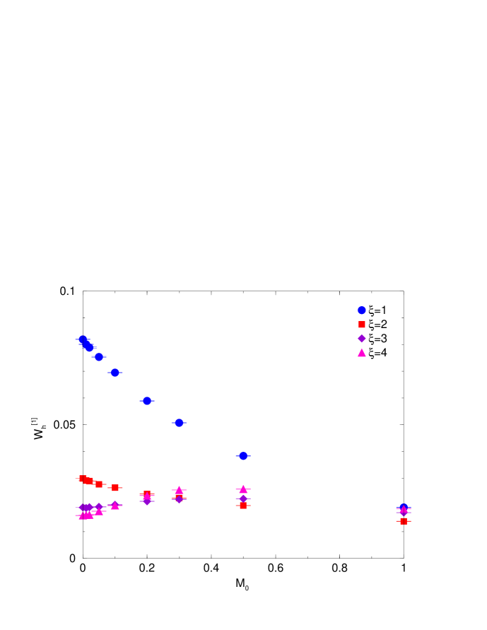
Figure 4: Mass dependence and $\xi$ dependence of the one-loop correction to the heavy quark wave function.

Here the introduction of anisotropy is seen to reduce the mass dependence greatly. Since $W_{h}^{[1]}$ connects smoothly to $W_{l}^{[1]}$, one sees that we have subtracted the infrared singularities in a consistent way.

Tables 4 and 5 list the one-loop corrections to the axial vector and the vector current vertex functions, respectively.

Table 4: The one-loop correction to the axial vector current vertex function.

	$M_{0}$	$\xi=1$	$\xi=2$	$\xi=3$	$\xi=4$
$V_{A_{4}}^{[1]}$	0.00	0.03449(1)	0.01005(1)	0.00033(1)	$-$0.00472(1)
	0.01	0.03425(13)	0.01028(17)	0.00071(10)	$-$0.00369(10)
	0.02	0.03399(10)	0.01061(10)	0.00134(8)	$-$0.00309(8)
	0.05	0.03426(8)	0.01145(7)	0.00337(6)	$-$0.00036(6)
	0.10	0.03435(6)	0.01294(5)	0.00628(5)	0.00399(5)
	0.20	0.03396(4)	0.01294(4)	0.01155(3)	0.01142(3)
	0.30	0.03389(4)	0.01543(4)	0.01585(3)	0.01717(3)
	0.50	0.03337(3)	0.02160(2)	0.02230(2)	0.02479(2)
	1.00	0.03309(2)	0.02818(2)	0.03187(2)	0.03465(1)
$V_{A_{i}}^{[1]}$	0.00	0.03450(1)	0.02669(1)	0.02460(1)	0.02454(1)
	0.01	0.03428(5)	0.02629(4)	0.02391(3)	0.02359(3)
	0.02	0.03410(3)	0.02602(3)	0.02352(2)	0.02294(2)
	0.05	0.03407(2)	0.02551(2)	0.02237(2)	0.02121(2)
	0.10	0.03378(2)	0.02463(2)	0.02075(1)	0.01896(1)
	0.20	0.03342(1)	0.02326(1)	0.01854(1)	0.01624(1)
	0.30	0.03302(1)	0.02223(1)	0.01716(1)	0.01490(1)
	0.50	0.03253(1)	0.02093(1)	0.01582(1)	0.01397(1)
	1.00	0.03176(1)	0.01950(1)	0.01512(1)	0.01429(1)

Table 5: The one-loop correction to the vector current vertex function.

	$M_{0}$	$\xi=1$	$\xi=2$	$\xi=3$	$\xi=4$
$V_{V_{4}}^{[1]}$	0.00	0.04749(1)	0.02071(1)	0.00695(1)	$-$0.00049(1)
	0.01	0.04740(13)	0.02036(11)	0.00641(10)	$-$0.00122(10)
	0.02	0.04677(10)	0.02021(9)	0.00641(9)	$-$0.00090(8)
	0.05	0.04690(8)	0.02006(6)	0.00631(6)	$-$0.00090(6)
	0.10	0.04628(7)	0.01957(6)	0.00622(5)	$-$0.00065(7)
	0.20	0.04532(5)	0.01904(4)	0.00617(3)	$-$0.00016(3)
	0.30	0.04404(4)	0.01815(3)	0.00611(3)	$-$0.00116(3)
	0.50	0.04165(3)	0.01669(3)	0.00579(2)	$-$0.00188(2)
	1.00	0.03629(3)	0.01308(2)	0.00439(2)	$-$0.00179(1)
$V_{V_{i}}^{[1]}$	0.00	0.04748(1)	0.04784(1)	0.04573(1)	0.04326(1)
	0.01	0.04727(4)	0.04764(4)	0.04570(3)	0.04320(3)
	0.02	0.04746(3)	0.04797(3)	0.04589(3)	0.04366(2)
	0.05	0.04779(2)	0.04843(2)	0.04665(2)	0.04436(2)
	0.10	0.04825(2)	0.04923(2)	0.04762(1)	0.04568(1)
	0.20	0.04917(1)	0.05075(1)	0.04967(1)	0.04807(1)
	0.30	0.05007(1)	0.05219(1)	0.05151(1)	0.05020(1)
	0.50	0.05175(1)	0.05481(1)	0.05467(1)	0.05369(1)
	1.00	0.05510(1)	0.05977(1)	0.06046(1)	0.05980(1)

The mass dependence is shown in Fig. 5 and 6.

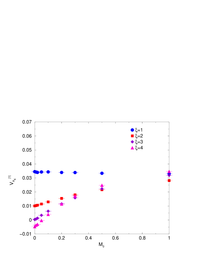
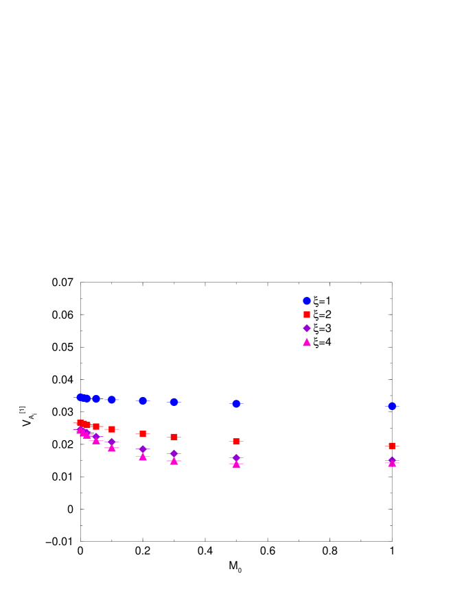
Figure 5: Mass dependence and $\xi$ dependence of the one-loop vertex corrections to the axial vector current.

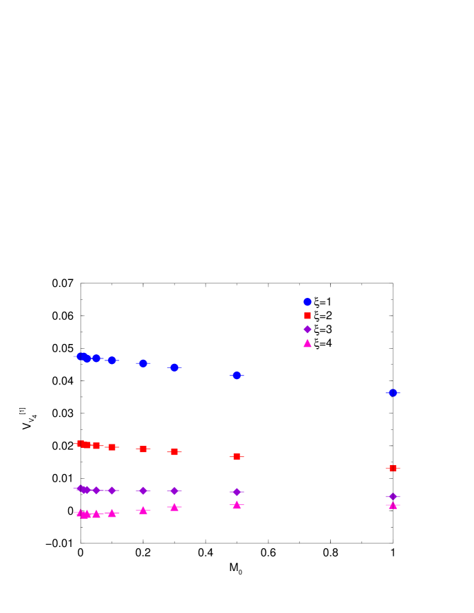
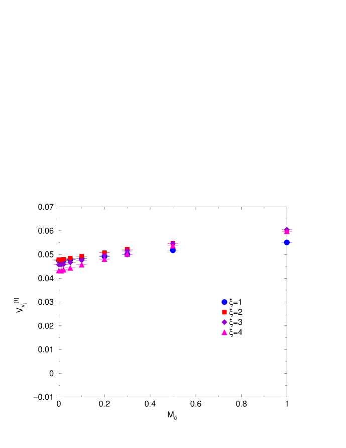
Figure 6: Mass dependence and $\xi$ dependence of the one-loop vertex corrections to the vector current.

For the axial vector current, the mass dependence with anisotropy is larger than with $\xi=1$, but still small.

These results are combined to obtain the one-loop part of the matching factors according to Eq. (3.33). The results are listed in Table 6 and plotted in Figs. 7 and 8.

Table 6: The one-loop term of the matching factor between the continuum and the lattice theories for the axial vector and the vector currents. The spatial and the temporal contributions are summed.

	$M_{0}$	$\xi=1$	$\xi=2$	$\xi=3$	$\xi=4$
$Z_{A_{4}}^{[1]}$	0.00	$-$0.11643(3)	$-$0.04000(3)	$-$0.01944(3)	$-$0.01133(2)
	0.01	$-$0.1153(2)	$-$0.0398(2)	$-$0.0197(2)	$-$0.0124(2)
	0.02	$-$0.1144(2)	$-$0.0400(2)	$-$0.0205(1)	$-$0.0131(1)
	0.05	$-$0.1129(2)	$-$0.0403(1)	$-$0.0226(1)	$-$0.0165(1)
	0.10	$-$0.1101(1)	$-$0.0412(1)	$-$0.02588(8)	$-$0.02192(9)
	0.20	$-$0.1044(1)	$-$0.04248(8)	$-$0.03178(6)	$-$0.03122(6)
	0.30	$-$0.1002(1)	$-$0.04423(8)	$-$0.03644(6)	$-$0.03800(5)
	0.50	$-$0.09351(8)	$-$0.04646(6)	$-$0.04302(5)	$-$0.04579(5)
	1.00	$-$0.08360(7)	$-$0.05009(5)	$-$0.04999(4)	$-$0.05196(4)
$Z_{A_{i}}^{[1]}$	0.00	$-$0.11644(3)	$-$0.05664(2)	$-$0.04371(2)	$-$0.04059(1)
	0.01	$-$0.1153(2)	$-$0.0558(1)	$-$0.04291(9)	$-$0.03972(9)
	0.02	$-$0.1145(1)	$-$0.05545(9)	$-$0.04267(8)	$-$0.03914(7)
	0.05	$-$0.1127(1)	$-$0.05436(8)	$-$0.04157(6)	$-$0.03807(6)
	0.10	$-$0.1095(1)	$-$0.05285(7)	$-$0.04035(5)	$-$0.03689(5)
	0.20	$-$0.10385(8)	$-$0.05032(5)	$-$0.03877(4)	$-$0.03604(4)
	0.30	$-$0.09935(7)	$-$0.04849(5)	$-$0.03776(4)	$-$0.03573(4)
	0.50	$-$0.09266(6)	$-$0.04580(4)	$-$0.03654(4)	$-$0.03497(3)
	1.00	$-$0.08227(5)	$-$0.04142(4)	$-$0.03324(4)	$-$0.03160(3)
$Z_{V_{4}}^{[1]}$	0.00	$-$0.12943(4)	$-$0.05066(2)	$-$0.02606(2)	$-$0.01556(3)
	0.01	$-$0.1284(2)	$-$0.0499(2)	$-$0.0254(2)	$-$0.0149(2)
	0.02	$-$0.1272(2)	$-$0.0496(2)	$-$0.0256(1)	$-$0.0153(1)
	0.05	$-$0.1256(2)	$-$0.0489(1)	$-$0.0255(1)	$-$0.0160(1)
	0.10	$-$0.1220(2)	$-$0.0478(1)	$-$0.02582(8)	$-$0.0173(1)
	0.20	$-$0.1158(1)	$-$0.04610(8)	$-$0.02640(7)	$-$0.01996(6)
	0.30	$-$0.1104(1)	$-$0.04442(7)	$-$0.02670(6)	$-$0.02199(6)
	0.50	$-$0.10178(8)	$-$0.04156(6)	$-$0.02651(5)	$-$0.02288(5)
	1.00	$-$0.08680(7)	$-$0.03499(5)	$-$0.02252(5)	$-$0.01910(4)
$Z_{V_{i}}^{[1]}$	0.00	$-$0.12942(3)	$-$0.07779(2)	$-$0.06484(2)	$-$0.05931(2)
	0.01	$-$0.1283(1)	$-$0.0772(1)	$-$0.06470(9)	$-$0.05933(9)
	0.02	$-$0.1279(1)	$-$0.07740(9)	$-$0.06503(8)	$-$0.05985(8)
	0.05	$-$0.1264(1)	$-$0.07728(8)	$-$0.06585(7)	$-$0.06121(6)
	0.10	$-$0.1240(1)	$-$0.07744(7)	$-$0.06721(5)	$-$0.06361(5)
	0.20	$-$0.11960(8)	$-$0.07781(5)	$-$0.06990(4)	$-$0.06787(4)
	0.30	$-$0.11639(8)	$-$0.07846(5)	$-$0.07211(4)	$-$0.07103(4)
	0.50	$-$0.11188(6)	$-$0.07968(4)	$-$0.07538(4)	$-$0.07469(3)
	1.00	$-$0.10561(5)	$-$0.08168(4)	$-$0.07859(4)	$-$0.07711(4)

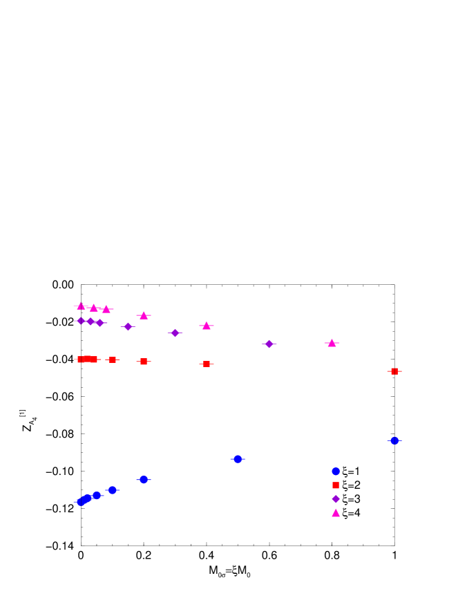
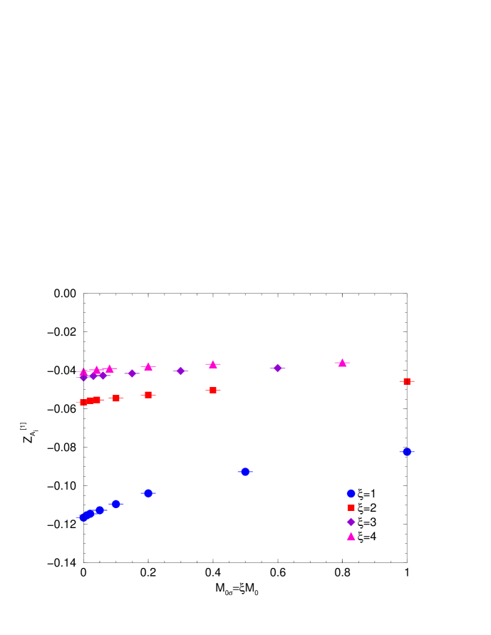
Figure 7: $Z_{A_{4}}^{[1]}$ and $Z_{A_{i}}^{[1]}$ vs. $M_{0\sigma}$.

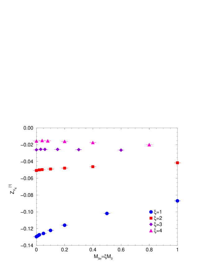
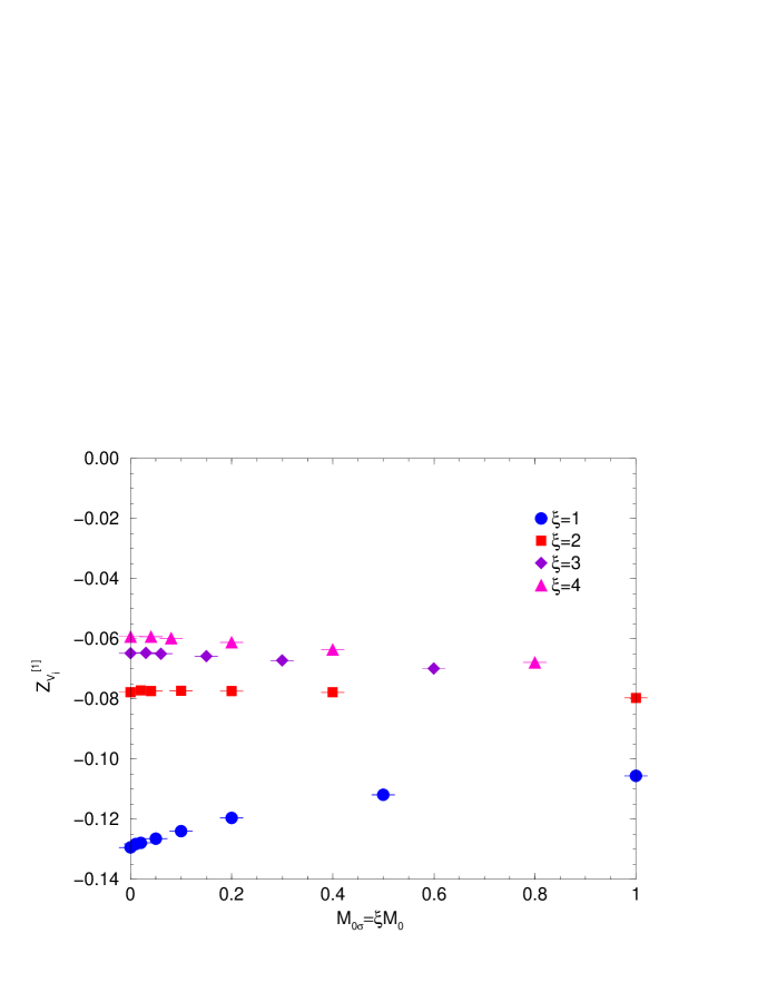
Figure 8: $Z_{V_{4}}^{[1]}$ and $Z_{V_{i}}^{[1]}$ vs. $M_{0\sigma}$.

The magnitude of the one-loop correction decreases as $\xi$ increases, in all cases. Figures 7 and 8 are the most important results of this section. They are relevant to phenomenological applications to charm physics. Moreover, these results test, at the one-loop level, whether the matching factors are well-behaved in the interesting region with small $M_{0}$ but $M_{0}\xi\sim 1$. For this reason we have plotted them, as in Fig. 1, not against $M_{0}$ but $M_{0}\xi$. By inspection of Figs. 7 and 8, one can see that the small $M_{0}$ Taylor series continues to be a good approximation to the full mass dependence for all $M_{0}\xi\leq 1$, for $\xi\geq 2$. Had we found a stronger mass dependence (like that of $\zeta^{[0]}$ for $r=1$), one would begin to doubt the feasibility of the ideas laid out in Ref. [4] also for our choice $r=1/\xi$.

For $\xi=1$, our results should reproduce previous calculations on isotropic lattices. In the case of the mass and the wave function renormalization, we (independently) reproduced the full mass dependence of Ref. [17]. For the matching factors of the currents, only the result for the massless quark is (independently) available [25], and we find agreement.

In conclusion, in the whole region of $M_{0}$ and $\xi$ we surveyed, we found good behavior connecting the continuum limit with the region of practical interest. For charmed hadrons, the target region of the heavy quark mass $M_{0}$ is around 0.1–0.3 on lattices with anisotropy $\xi$=3–4. The required one-loop coefficients of the renormalization factors are easily obtained by interpolating the values in the tables using, for example, spline interpolation.

5 Conclusion

In this paper, we have studied the $O(a)$ improvement of Wilson quarks on anisotropic lattices. At the tree-level we find that a certain choice of the parameters, $r=1/\xi$ [9, 10], is well-behaved in the region of practical interest for charmed hadrons, namely $M_{0}a_{\sigma}\sim 1$, while $M_{0}a_{\tau}$ is small. On the other hand, with a different choice, $r=1$ [4, 11, 12], continuum behavior is reached only for $M_{0}a_{\sigma}\ll 1$. With this latter choice a non-relativistic interpretation [6, 7] is still possible, but a mass-independent renormalization, which was proposed in Ref. [4], is obstructed.

The choice $r=1/\xi$ also simplifies tree-level $O(a)$ improvement. The action does not require separate temporal and spatial hopping parameters. The currents require mass-dependent matching factors, but no intrinsically dimension-four terms.

We therefore have started to examine the behavior of this choice at the one-loop level. We have computed the one-loop contributions to the rest mass and to the matching factors of the vector and axial vector currents. The matching factors depend significantly on $\xi$. A more critical observation is that they are well approximated by Taylor expansions

$$Z_{J_{\Gamma}}(\xi,M_{0}a_{\tau})\simeq Z_{J_{\Gamma}}(\xi,0)+M_{0}a_{\tau}Z^{\prime}_{J_{\Gamma}}(\xi,0)$$ (5.1)

for $M_{0}a_{\sigma}=\xi M_{0}a_{\tau}\leq 1$ and $\xi=2$–$4$. This region encompasses the one suitable for the charmed quark with currently available computer resources.

There are several issues that remain to be studied. The first is to compute the one-loop corrections to the ratio of hopping parameters $\zeta$, the clover coefficients $c_{B}$ and $c_{E}$, and dimension-four terms in the currents. The calculation of $\zeta$ is especially difficult, because it requires the one-loop kinetic mass $M_{2}^{[1]}$. As at the tree-level, it is crucial to compute the full mass dependence, so one can check whether low-order Taylor expansions work well for $M_{0}a_{\sigma}\sim 1$. Only with the full mass dependence can one check whether $\xi$, which comes with the couplings in the action, and $M_{0}a_{\tau}$, which also comes from the on-shell condition, come together to form $M_{0}a_{\sigma}=\xi M_{0}a_{\tau}$. If not, then one could proceed with a non-perturbative calculation of $\zeta(\xi,0)$, $\zeta^{\prime}(\xi,0)$, $c_{B}(\xi,0)$, $c_{E}(\xi,0)$, etc.

A more practical problem is to define renormalized couplings. The scale-setting scheme of Brodsky, Lepage, and Mackenzie (BLM) is usually a good way to absorb the dominant part of two- and higher-order contributions [26, 22]. On an anisotropic lattice, it may make sense to define separate scales for temporal and spatial gluons. These results are of interest in any case: even if anisotropic lattice calculations require a non-relativistic interpretation for heavy quarks, anisotropy remains a useful tool for improving the signal-to-noise ratio.

Finally, after these problems are resolved, it will be important to combine the results with numerical simulation data to obtain the matrix elements relevant to experimental measurements of charmed hadrons.

Appendix A Feynman rules

(a)  ${\cal V}^{\rm(MF)}_{4}(p)$                                  (b)  ${\cal V}^{\rm(MF)}_{\sigma}(p)$

Figure 9: Feynman rules required for the one-loop perturbation theory.

The Feynman rules for perturbative calculation are shown the same as in Ref. [17] except for two points. One is that the $c_{B}$ is replaced by $r_{s}c_{B}$ as was mentioned in Sec. 2.1 and the other is the gluon propagator. With a gauge fixing term that is symmetric under exchange of temporal and spatial axis, the free propagator of the gauge field, in Feynman gauge, is

$$G_{\mu\nu}(k)=\left\{\begin{array}[]{ll}G_{\tau}(k){}{}&\mu=\nu=4\\ G_{\sigma}(k)&\mu=\nu<4\\ 0&\mu\neq\nu\end{array}\right.$$ (A.1)

$$G_{\sigma} = \frac{\delta_{ab}\xi}{\hat{k}_{i}^{2}+\xi^{2}\hat{k}_{4}^{2}+\xi^{2}\lambda^{2}},$$

$$G_{\tau} = \frac{1}{\xi^{2}}G_{\sigma}(k).$$ (A.2)

where we replaced the anisotropy parameter $\gamma_{G}$ with the tree-level value $\xi$. A fictitious gluon mass $\lambda$ is introduced to regulate infrared divergences.

The Feynman diagram for the counter-term from the mean field is obtained by expanding

$$u_{\tau} = 1+g^{2}u_{\tau}^{[1]}+O(g^{4}),$$ (A.3)

$$u_{\sigma} = 1+g^{2}u_{\sigma}^{[1]}+O(g^{4}).$$ (A.4)

With the replacement of the link variables as Eq. (3.21) in the action (2.5), the Feynman rules required for the the one-loop calculation are

$${\cal V}^{\rm(MF)}_{4}(p) = g^{2}u_{\tau}^{[1]}[\gamma_{4}i\sin p_{4}-\cos p_{4}]$$ (A.5)

$${\cal V}^{\rm(MF)}_{\sigma}(p) = g^{2}u_{\sigma}^{[1]}\sum_{j}[\zeta\gamma_{j}i\sin p_{j}-r\zeta\cos p_{j}]$$ (A.6)

with the diagrams (a) and (b) in Fig. 9, respectively.

Appendix B Explicit expressions of one-loop corrections

In the following, we show the explicit representations of the self-energy and the vertex correction. In order to simplify the expressions, we introduce the following abbreviations:

$$c_{\mu} = \cos k_{\mu},\hskip 62.59596pts_{\mu}=\sin k_{\mu},$$

$$\check{c}_{\mu} = \cos\left({\textstyle\frac{1}{2}}k_{\mu}\right),\hskip 45.52458pt\check{s}_{\mu}=\sin\left({\textstyle\frac{1}{2}}k_{\mu}\right),$$

$$C_{4} = \cos(iM_{1}+k_{4}),\hskip 25.6073ptS_{4}=\sin(iM_{1}+k_{4}),$$

$$\check{C}_{4} = \cos\left(iM_{1}+{\textstyle\frac{1}{2}}k_{4}\right),\hskip 14.22636pt\check{S}_{4}=\sin\left(iM_{1}+{\textstyle\frac{1}{2}}k_{4}\right).$$ (B.1)

$$\mbox{\boldmath$s$}^{2}=\sum_{i=1}^{3}s_{i}s_{i},\hskip 28.45274pt\check{\mbox{\boldmath$c$}}^{2}=\sum_{i=1}^{3}\check{c}_{i}\check{c}_{i},\hskip 28.45274pt[\mbox{\boldmath$s$}\cdot\check{\mbox{\boldmath$c$}}]=\sum_{i=1}^{3}s_{i}^{2}\check{c}_{i}^{2}.$$ (B.2)

To reduce the volume of notation, we also define

$$c^{\prime}_{B}=r\zeta c_{B},\hskip 28.45274ptc^{\prime}_{E}=rc_{E},$$ (B.3)

which always appear in these combinations. To reduce the Dirac matrix structure, it is convenient to introduce $G^{Q}=\pm 1$, with the upper (lower) sign for massive quarks (anti-quarks) on the external leg, and $G$ and $H$, defined by

$$G\Gamma=\gamma_{4}\Gamma\gamma_{4},\quad H\Gamma=\gamma^{\mu}\Gamma\gamma_{\mu},$$ (B.4)

with an implied sum on $\mu$. The following quantities are convenient for representing the one-loop expressions below and in our integration programs:

$$A^{q} = -iG\check{c}_{4}-\check{s}_{4},\hskip 69.70915ptA^{Q}=-iG^{Q}\check{C}_{4}-\check{S}_{4},$$ (B.5)

$$B^{q} = -iG{s}_{4}+2\check{s}_{4}^{2}+2r\zeta\check{\mbox{\boldmath$s$}}^{2},\hskip 22.76228ptB^{Q}=-iG^{Q}{S}_{4}+1+m_{0}-C_{4}+2r\zeta\check{\mbox{\boldmath$s$}}^{2},$$ (B.6)

$$E^{q} = -i\zeta+{\textstyle\frac{1}{2}}c^{\prime}_{E}Gs_{4},\hskip 54.06006ptE^{Q}=-i\zeta+{\textstyle\frac{1}{2}}c^{\prime}_{E}G^{Q}S_{4},$$ (B.7)

$$J^{q} = -iGc_{4}+s_{4},\hskip 68.28644ptJ^{Q}=-iG^{Q}C_{4}+S_{4},$$ (B.8)

and

$$\bar{B}^{q} = iG{s}_{4}+2\check{s}_{4}^{2}+2r\zeta\check{\mbox{\boldmath$s$}}^{2},\hskip 22.76228pt\bar{B}^{Q}=iG^{Q}{S}_{4}+1+m_{0}-C_{4}+2r\zeta\check{\mbox{\boldmath$s$}}^{2},$$ (B.9)

$$\bar{J}^{q} = iGc_{4}+s_{4},\hskip 68.28644pt\bar{J}^{Q}=iG^{Q}C_{4}+S_{4}.$$ (B.10)

The symbols with superscript $q$ are essentially massless versions of those with superscript $Q$.

From the Feynman rules in Appendix A, the contributions to the self-energy from the rainbow diagram, Fig. 2(a), are

$$\Sigma_{a}(iM_{1},{\bf 0}) = g^{2}_{\sigma}\Sigma_{a\sigma}^{[1]}(iM_{1},{\bf 0})+g^{2}_{\tau}\Sigma_{a\tau}^{[1]}(iM_{1},{\bf 0})+O(g^{4}),$$ (B.11)

$$\Sigma_{a\sigma}^{[1]}(iM_{1},{\bf 0}) = C_{F}\int\frac{d^{4}k}{(2\pi)^{4}}S_{Q}(iM_{1}+k_{4},\mbox{\boldmath$k$})G_{\sigma}(k)\left[\check{\mbox{\boldmath$c$}}^{2}\bar{B}^{Q}(E^{Q})^{2}+r^{2}\zeta^{2}\check{\mbox{\boldmath$s$}}^{2}B^{Q}\right.$$ (B.12)

$$\hskip 42.67912pt\left.+ir\zeta^{2}\mbox{\boldmath$s$}^{2}E^{Q}+\left(i\zeta c^{\prime}_{B}E^{Q}+{\textstyle\frac{1}{4}}c_{B}^{\prime 2}B^{Q}\right)\left(\mbox{\boldmath$s$}^{2}\check{\mbox{\boldmath$c$}}^{2}-[\mbox{\boldmath$s$}\cdot\check{\mbox{\boldmath$c$}}]\right)\right],$$

$$\Sigma_{a\tau}^{[1]}(iM_{1},{\bf 0}) = C_{F}\int\frac{d^{4}k}{(2\pi)^{4}}S_{Q}(iM_{1}+k_{4},\mbox{\boldmath$k$})G_{\tau}(k)$$ (B.13)

$$\hskip 56.9055pt\times\left[(A^{Q})^{2}B^{Q}+\mbox{\boldmath$s$}^{2}\left(i\zeta c^{\prime}_{E}\check{c}_{4}A^{Q}G^{Q}+{\textstyle\frac{1}{4}}c_{E}^{\prime 2}\check{c}_{4}^{2}\bar{B}^{Q}\right)\right].$$

where

$$S_{Q}(p)=\left[\sin^{2}p_{4}+\zeta^{2}\sum_{j}\sin^{2}p_{j}+\left\{{\textstyle\frac{1}{2}}(\hat{p}_{4}^{2}+r\zeta\hat{\mbox{\boldmath$p$}}^{2})+m_{0}\right\}^{2}\right]^{-1}.$$ (B.14)

Similarly, the contributions from the tadpole diagram, Fig. 2(b), are

$$\Sigma_{b}(iM_{1},{\bf 0}) = g^{2}_{\sigma}\Sigma_{b\sigma}^{[1]}(iM_{1},{\bf 0})+g^{2}_{\tau}\Sigma_{b\tau}^{[1]}(iM_{1},{\bf 0})+O(g^{4}),$$ (B.15)

$$\Sigma_{b\sigma}^{[1]}(iM_{1},{\bf 0}) = -{\textstyle\frac{1}{2}}C_{F}\int\frac{d^{4}k}{(2\pi)^{4}}G_{\sigma}(k)3r\zeta,$$ (B.16)

$$\Sigma_{b\tau}^{[1]}(iM_{1},\mbox{\bf 0}) = -{\textstyle\frac{1}{2}}C_{F}\int\frac{d^{4}k}{(2\pi)^{4}}G_{\tau}(k)\left(G^{Q}\sinh M_{1}+\cosh M_{1}\right).$$ (B.17)

The derivative of the self-energy with respective to $p_{4}$ is separated into temporal and spatial contributions

$$\dot{\Sigma}(iM_{1},{\bf 0})=g^{2}_{\sigma}\dot{\Sigma}_{\sigma}^{[1]}(iM_{1},\mbox{\bf 0})+g^{2}_{\tau}\dot{\Sigma}_{\tau}^{[1]}(iM_{1},\mbox{\bf 0})+O(g^{4})$$ (B.18)

The contributions from Fig. 2(a) are

$$\dot{\Sigma}_{a\sigma}^{[1]}(iM_{1},\mbox{\bf 0}) = -iC_{F}\int\frac{d^{4}k}{(2\pi)^{4}}G_{\sigma}(k)\left[-2S_{Q}(iM_{1}+k_{4},\mbox{\boldmath$k$})^{2}S_{4}\left(1+2r\zeta\check{\mbox{\boldmath$s$}}^{2}+m_{0}\right)\right.$$

$$\times\left\{\check{\mbox{\boldmath$c$}}^{2}(E^{Q})^{2}\bar{B}^{Q}+r^{2}\zeta^{2}\check{\mbox{\boldmath$s$}}^{2}B^{Q}+ir\zeta^{2}\mbox{\boldmath$s$}^{2}E^{Q}+\left(i\zeta c^{\prime}_{B}E^{Q}+{\textstyle\frac{1}{4}}c_{B}^{\prime 2}B^{Q}\right)\left(\mbox{\boldmath$s$}^{2}\check{\mbox{\boldmath$c$}}^{2}-[\mbox{\boldmath$s$}\cdot\check{\mbox{\boldmath$c$}}]\right)\right\}$$

$$\left.+S_{Q}(iM_{1}+k_{4},\mbox{\boldmath$k$})\left\{\check{\mbox{\boldmath$c$}}^{2}(E^{Q})^{2}\bar{J}^{Q}+r^{2}\zeta^{2}\check{\mbox{\boldmath$s$}}^{2}J^{Q}+{\textstyle\frac{1}{4}}c_{B}^{\prime 2}(\mbox{\boldmath$s$}^{2}\check{\mbox{\boldmath$c$}}^{2}-[\mbox{\boldmath$s$}\cdot\check{\mbox{\boldmath$c$}}])J^{Q}\right\}\right]$$

$$\dot{\Sigma}_{a\tau}^{[1]}(iM_{1},\mbox{\bf 0}) = -iC_{F}\int\frac{d^{4}k}{(2\pi)^{4}}G_{\tau}(k)\left[-2S_{Q}(iM_{1}+k_{4},\mbox{\boldmath$k$})^{2}S_{4}\left(1+2r\zeta\check{\mbox{\boldmath$s$}}^{2}+m_{0}\right)\right.$$

$$\times\left\{(A^{Q})^{2}B^{Q}+\mbox{\boldmath$s$}^{2}\left(i\zeta c^{\prime}_{E}\check{c}_{4}A^{Q}G^{Q}+{\textstyle\frac{1}{4}}c_{E}^{\prime 2}\check{c}_{4}^{2}\bar{B}^{Q}\right)\right\}$$

$$+S_{Q}(iM_{1}+k_{4},\mbox{\boldmath$k$})\left.\left\{-2i(A^{Q})^{2}B^{Q}G^{Q}+\zeta c^{\prime}_{E}\check{c}_{4}\mbox{\boldmath$s$}^{2}A^{Q}+{\textstyle\frac{1}{4}}c_{E}^{\prime 2}\check{c}_{4}^{2}\mbox{\boldmath$s$}^{2}\bar{J}^{Q}+(A^{Q})^{2}J^{Q}\right\}\right].$$

There is only one contribution from Fig. 2(b)

$$\dot{\Sigma}_{b}^{[1]}(iM_{1},{\bf 0})=-{\textstyle\frac{i}{2}}C_{F}\int\frac{d^{4}k}{(2\pi)^{4}}G_{\tau}(k)[G^{Q}\cosh M_{1}+\sinh M_{1}],$$ (B.21)

with a temporal gluon.

The vertex function is split as follows:

$$g^{2}\Lambda_{\Gamma}^{[1]}=g^{2}_{\sigma}\Lambda^{[1]}_{\Gamma\sigma}+g^{2}_{\tau}\Lambda^{[1]}_{\Gamma\tau},$$ (B.22)

and the contributions are

$$\Lambda^{[1]}_{\Gamma\sigma} = C_{F}\int\frac{d^{4}k}{(2\pi)^{4}}S_{Q}(iM_{1}+k_{4},\mbox{\boldmath$k$})S_{q}(k)G_{\sigma}(k)\left[\frac{1}{3}\check{\mbox{\boldmath$c$}}^{2}(H-G)E^{q}\overline{B}^{q}E^{Q}\overline{B}^{Q}\right.$$ (B.23)

$$\hskip 22.76228pt+\,\frac{i}{6}\zeta(H-G)\left\{c^{\prime}_{B}(\mbox{\boldmath$s$}^{2}\check{\mbox{\boldmath$c$}}^{2}-[\mbox{\boldmath$s$}\cdot\check{\mbox{\boldmath$c$}}])+r\zeta\mbox{\boldmath$s$}^{2}\right\}(E^{q}\overline{B}^{q}+\overline{B}^{Q}E^{Q})$$

$$\hskip 22.76228pt+\,{\textstyle\frac{i}{2}}\zeta\left\{\frac{1}{6}c^{\prime}_{B}(\mbox{\boldmath$s$}^{2}\check{\mbox{\boldmath$c$}}^{2}-[\mbox{\boldmath$s$}\cdot\check{\mbox{\boldmath$c$}}])\left((H-G)^{2}-3\right)+r\zeta\mbox{\boldmath$s$}^{2}\right\}(E^{q}B^{Q}+B^{q}E^{Q})$$

$$\hskip 22.76228pt+\,\left\{\frac{1}{24}c_{B}^{\prime 2}(\mbox{\boldmath$s$}^{2}\check{\mbox{\boldmath$c$}}^{2}-[\mbox{\boldmath$s$}\cdot\check{\mbox{\boldmath$c$}}])\Big{(}(H-G)^{2}-3\Big{)}+r^{2}\zeta^{2}\check{\mbox{\boldmath$s$}}^{2}\right\}B^{q}B^{Q}$$

$$\hskip 22.76228pt-\,\zeta^{2}\left\{\frac{1}{6}(\mbox{\boldmath$s$}^{2}\check{\mbox{\boldmath$c$}}^{2}-[\mbox{\boldmath$s$}\cdot\check{\mbox{\boldmath$c$}}])\left((H-G)^{2}-3\right)+[\mbox{\boldmath$s$}\cdot\check{\mbox{\boldmath$c$}}]\right\}E^{q}E^{Q}$$

$$\hskip 22.76228pt\left.-\,\frac{1}{12}c_{B}^{\prime 2}\zeta^{2}\mbox{\boldmath$s$}^{2}(\mbox{\boldmath$s$}^{2}\check{\mbox{\boldmath$c$}}^{2}-[\mbox{\boldmath$s$}\cdot\check{\mbox{\boldmath$c$}}])(H-G)-\frac{1}{3}r^{2}\zeta^{4}\mbox{\boldmath$s$}^{2}\check{\mbox{\boldmath$s$}}^{2}(H-G)\right]\Gamma,$$

$$\Lambda^{[1]}_{\Gamma\tau} = C_{F}\int\frac{d^{4}k}{(2\pi)^{4}}S_{Q}(iM_{1}+k_{4},\mbox{\boldmath$k$})S_{q}(k)G_{\tau}(k)\times$$ (B.24)

$$\hskip 17.07182pt\left[\Big{(}A^{q}B^{q}+{\textstyle\frac{i}{2}}\zeta c^{\prime}_{E}\check{c}_{4}\mbox{\boldmath$s$}^{2}G\Big{)}\Big{(}A^{Q}B^{Q}+{\textstyle\frac{i}{2}}\zeta c^{\prime}_{E}\check{c}_{4}\mbox{\boldmath$s$}^{2}G^{Q}\Big{)}\right.$$

$$\hskip 22.76228pt\left.+\frac{1}{3}(H-G)\mbox{\boldmath$s$}^{2}\Big{(}i\zeta A^{q}+{\textstyle\frac{1}{2}}c^{\prime}_{E}\check{c}_{4}\overline{B}^{q}G\Big{)}\Big{(}i\zeta A^{Q}+{\textstyle\frac{1}{2}}c^{\prime}_{E}\check{c}_{4}\overline{B}^{Q}G^{Q}\Big{)}\right]\Gamma.$$

References

-
[1]
F. Karsch,
Nucl. Phys. B 205 (1982) 285;
G. Burgers, F. Karsch, A. Nakamura, and I. O. Stamatescu, ibid. 304 (1988) 587. - [2] C. J. Morningstar and M. J. Peardon, Phys. Rev. D 56 (1997) 4043; 60 (1999) 034509.
-
[3]
J. Fingberg,
Phys. Lett. B 424 (1998) 343;
K. J. Juge, J. Kuti, and C. J. Morningstar, Nucl. Phys. B Proc. Suppl. 63 (1998) 543; Phys. Rev. Lett. 82 (1999) 4400; Nucl. Phys. B Proc. Suppl. 83 (2000) 304;
I. T. Drummond, R. R. Horgan, T. Manke, and H. P. Shanahan, Nucl. Phys. B Proc. Suppl. 73 (1999) 336;
T. Manke et al. [CP-PACS Collaboration], Phys. Rev. Lett. 82 (1999) 4396; Nucl. Phys. B Proc. Suppl. 86 (2000) 397;
I. T. Drummond et al., Phys. Lett. B 478 (2000) 151;
S. Collins et al., hep-lat/0101019. - [4] T. R. Klassen, Nucl. Phys. B 509 (1998) 391; Nucl. Phys. B Proc. Suppl. 73 (1999) 918.
-
[5]
G. P. Lepage and B. A. Thacker,
Nucl. Phys. B Proc. Suppl. 4, 199 (1987);
B. A. Thacker and G. P. Lepage, Phys. Rev. D 43, 196 (1991);
G. P. Lepage, L. Magnea, C. Nakhleh, U. Magnea, and K. Hornbostel, ibid. 46, 4052 (1992). - [6] A. X. El-Khadra, A. S. Kronfeld, and P. B. Mackenzie, Phys. Rev. D 55 (1997) 3933.
- [7] A. S. Kronfeld, Phys. Rev. D 62 (2000) 014505.
-
[8]
K. Jansen et al.,
Phys. Lett. B 372 (1996) 275;
M. Lüscher, S. Sint, R. Sommer, P. Weisz, and U. Wolff, Nucl. Phys. B 491 (1997) 323. - [9] Ph. de Forcrand et al. [QCD-TARO Collaboration], Nucl. Phys. B Proc. Suppl. 83 (2000) 411.
- [10] T. Umeda, R. Katayama, O. Miyamura, and H. Matsufuru, hep-lat/0011085 (to appear in Int. J. Mod. Phys.).
-
[11]
P. Chen, hep-lat/0006019;
P. Chen, X. Liao, and T. Manke, Nucl. Phys. B Proc. Suppl. 94 (2001) 342. - [12] A. Ali Khan et al. [CP-PACS Collaboration], Nucl. Phys. B Proc. Suppl. 94 (2001) 325.
- [13] S. Groote and J. Shigemitsu, Phys. Rev. D 62 (2000) 014508.
- [14] K. G. Wilson, in New Phenomena in Subnuclear Physics, edited by A. Zichichi (Plenum, New York, 1977).
- [15] B. Sheikholeslami and R. Wohlert, Nucl. Phys. B 259 (1985) 572.
- [16] M. Okamoto, unpublished.
- [17] B. P. G. Mertens, A. S. Kronfeld, and A. X. El-Khadra, Phys. Rev. D 58 (1998) 034505.
- [18] Y. Kuramashi, Phys. Rev. D 58 (1998) 034507.
-
[19]
K.-I. Ishikawa, S. Aoki, S. Hashimoto, H. Matsufuru, T. Onogi,
and N. Yamada,
Nucl. Phys. B Proc. Suppl. 63, (1998) 344;
K.-I. Ishikawa, T. Onogi, and N. Yamada, Nucl. Phys. B Proc. Suppl. 83, (2000) 301. - [20] J. Harada et al., to appear.
- [21] A. S. Kronfeld, Phys. Rev. D 58 (1998) 051501.
- [22] G. P. Lepage and P. B. Mackenzie, Phys. Rev. D 48 (1993) 2250.
-
[23]
G. Heatlie et al.,
Nucl. Phys. B 352 (1991) 266;
M. Lüscher, S. Sint, R. Sommer, and P. Weisz, Nucl. Phys. B 478 (1996) 365. - [24] S. Kawabata, Comput. Phys. Commun. 88 (1995) 309.
- [25] S. Aoki, K. Nagai, Y. Taniguchi, and A. Ukawa, Phys. Rev. D 58 (1998) 074505.
- [26] S. J. Brodsky, G. P. Lepage and P. B. Mackenzie, Phys. Rev. D 28 (1983) 228.