From Surface Roughening to QCD String Theory

Abstract

Surface critical phenomena and the related onset of Goldstone modes represent fundamental properties of the confining flux in Quantum Chromodynamics. New ideas on surface roughening and their implications for lattice studies of quark confinement and string formation are presented. Problems with a simple string description of the large Wilson surface are discussed.

1 Introduction

There exists great interest and considerable effort to explain quark confinement in Quantum Chromodynamics (QCD) from the string theory viewpoint. The ideas of ’t Hooft, Polyakov, Witten, and others, and recent glueball spectrum or QCD string tension calculations in AdS theories are some illustrative examples of these activities. In a somewhat complementary approach, the search for a microscopic mechanism to explain quark confinement in the QCD vacuum continues with vigorous effort. It is useful to note (in loose chronological order) some of the ideas on QCD string formation:

(i)

The strong coupling lattice picture. This is the oldest “string-like” confinement picture which was formulated in the early days of lattice QCD and immediately raised the issue of the surface roughening transition on a large area Wilson loop.

(ii)

Microscopic confinement mechanisms. To understand confinement as we move past the roughening transition from strong coupling towards the continuum limit, on-lattice (and off-lattice) ideas were developed about microscopic confinement mechanisms in the QCD vacuum. Candidates of dominant gauge field configurations include instantons, monopoles, Z(N) flux configurations, and other examples. A popular idea is based on dual superconductivity with magnetic monopoles playing the dominant role in an underlying effective Landau-Ginzburg type low energy theory of the confining flux.

(iii)

Large N expansion. ’t Hooft suggested that in the large N limit of nonabelian SU(N) gauge theories, the summation of the leading diagrams might lead to the expected QCD string picture of quark confinement. This idea is very powerful and remains much studied today in various settings.

(iv)

QCD in loop space formulation. Polyakov reformulated the path integral approach to nonabelian Yang-Mills fields with the hope that “string-like” microscopic variables will help to understand the emergence of the confining string.

(v)

Confinement from higher dimensions. This very popular idea is based on the higher dimensional Anti-deSitter (AdS) space and one of its ambitious goals is to the understand the origin of quark confinement.

(vi)

Surface spectrum and D=2 conformal field theory. We will argue that a deeper understanding of the string theory connection with large Wilson surfaces will require a more precise knowledge of the surface excitation spectrum and the determination of the appropriate universality class of surface criticality. This new QCD string universality class will also require a consistent description of the conformal properties of the gapless surface excitation spectrum.

2 Lattice Study of QCD String Formation: Three Objectives

In this progress report we present our ab initio on-lattice calculations to probe the dynamics of string formation in QCD when the separation of the static quark-antiquark pair at the two ends of the confining flux becomes large. Our view is that the relevant properties of the underlying effective QCD string theory, whether it emerges from strictly string theoretic ideas, or from the microscopic theory of the confining vacuum, are coded in the excitation spectrum of the confining flux. To establish the main features of this spectrum remains our main objective. In collaboration with Mike Peardon[3], we are also developing the relevant methodology to study the spectrum of a “closed” flux loop across periodic slab geometry (Polyakov line) by choosing appropriate boundary conditions and operators for selected excitations of the flux without static sources.

Throughout this work we will focus on the confining properties of the nonabelian Yang-Mills field and the effects of light quark vacuum polarization will be neglected. Since this is an interim progress report, we will focus only on the results of the calculations and their physical interpretation. The technical details will be completely omitted. Acting within space and time limitations, we will be unable to provide appropriate references to the literature. These omissions will be remedied in our forthcoming publications. As reported here in the next three sections, the main thrust of our recent work develops along three closely related lines of investigations:

    

Section 3: The Excitation Spectrum of the Wilson Surface in QCD.
After building a Beowolf class UP2000 Alpha cluster with 9.33 Gflops computing power,[5] dedicated to this project, we increased the statistics of our earlier work on the excitation spectrum of the Wilson surface by more than an order of magnitude. We determined the spectrum as the function of the ${\rm Q\overline{Q}}$ separation and established three well identified scales of the confining flux. We also found that the main features of string formation share some universal properties, independent of the tested gauge groups SU(2) and SU(3), and the tested space-time dimensions D=3 and D=4.

    

Section 4: Surface Excitation Spectrum in Z(2) Spin and Gauge Models.
A quantitative analysis of the exact surface excitation spectrum and its conformal properties are presented for the BCSOS model in three dimensions. From the Bethe Ansatz equations we calculate numerically the exact spectrum of the interface using transfer matrix methods. We also interpret this spectrum in two-dimensional conformal field theory. The surface physics of the Z(2) gauge model is closely related to the BCSOS model by universality argument and a duality transformation. The string limit of the confining flux in the Z(2) model will be discussed in the critical region of the bulk. New issues will be raised about the crossover behavior of the confining Wilson surface in the Z(2) gauge model as we move from the roughening transition into the critical domain of the bulk embedding medium of the surface. Some puzzling features remain unresolved as we progress.

    

Section 5: What Is the Continuum Limit of QCD String Theory?
The intricate connection between the on-lattice roughening transition of the Wilson surface and the crossover to continuum string behavior will be discussed in ${\rm QCD_{3}}$. Based on the investigation of the Z(2) gauge model, we describe the important crossover issue as we move from the roughening transition point of the Wilson surface towards the critical domain of the gauge theory vacuum which represents the bulk embedding medium for the Wilson surface in the continuum limit. We will raise the question whether the universality class of the Wilson surface in the continuum is different from the Kosterlitz-Thouless universality class of the surface at the roughening transition.

3 The Excitation Spectrum of the Wilson Surface in QCD

A rather comprehensive determination of the rich energy spectrum of the gluon excitations

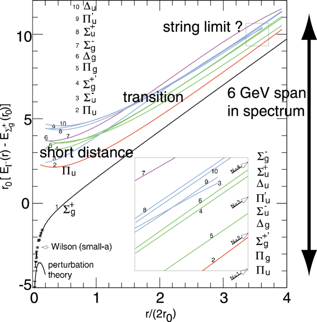
Figure 1: Continuum limit extrapolations are shown for the excitation energies where an arbitrary constant is removed by subtraction. Color coding in postscript is added to the numerical labelling of the excitations (N=0,black:1), (N=1,red:2), (N=2,green:4,5,6), (N=3,blue:3,8,9,10), and (N=4,cyan:7). The five groups represent the expected quantum numbers of a string in its ground state (N=0) and the first four excited states (N=1,2,3,4). The arrows in the inset represent the expected locations of the four lowest massless string excitations (N=1,2,3,4) which have to be compared with the energy levels of our computer simulations.

between static sources in the fundamental representation of ${\rm SU(3)_{c}}$ in D=4 dimensions was reported earlier[1, 2] for quark-antiquark separations r ranging from 0.1 fm to 4 fm.

The extrapolation of the full spectrum to the continuum limit is summarized in Fig. 1 with very different characteristic behavior on three separate physical scales. Error bars are not shown, and the earlier results displayed here remain compatible with our new run on the UP2000 Alpha cluster after more than a tenfold increase in statistics (a Bayesian statistical analysis on the new results is in progress). Our notation and the origin of the quantum numbers used in the classification of the energy levels are explained in the Appendix. Following Sommer[8], the physical scale ${\rm r_{0}}$ in Fig. 1 is set by the relation

$${\rm[r^{2}dE_{\Sigma^{+}_{\rm g}}(\vec{r})/dr]}_{\rm r=r_{0}}=1.65~{}.$$ (1)

This scale turns out to be ${\rm r_{0}=0.5~{}fm}$ to a good approximation.

The full spectrum, determined as a function of quark-antiquark separation, spans over 6 GeV in energy range which requires rather sophisticated lattice technology. Qualitatively, we can identify three distinct regions in the spectrum. Nontrivial short distance physics dominates for $r\leq 0.3~{}{\rm fermi}$. The transition region towards string formation is identified on the scale $0.5~{}{\rm fm}\leq 2.0~{}{\rm fm}$. String formation and the onset of string-like ordering of the excitation energies occurs in the range between 2 fm and 4 fm which is the current limit of our technology.

3.1 Short Distance Physics

The observed energy levels, even their qualitative ordering, are in violent disagreement with naive expectations from a fluctuating string for quark-antiquark separations ${\rm r\leq 2~{}fm}$. It is not difficult to show that for small ${\rm r\leq 0.3~{}\rm fm}$ the non-string level ordering is consistent with the short distance operator product expansion (OPE) around static color sources for gluon excitations. Consider the static QCD Hamiltonian in Coulomb gauge,

$${\rm H_{Cb}=H_{gluon}+\frac{g^{2}Q\cdot\overline{Q}}{4\pi\mid\vec{r}_{1}-\vec{r}_{2}\mid}-g^{3}(Q\times\overline{Q})_{a}\int d^{3}r\vec{A}_{a}(\vec{r},t)\vec{J}(\vec{r})}$$ (2)

where the intrinsic color operator ${\rm Q\cdot\overline{Q}}$ takes the value -4/3 for a color singlet pair, and 1/6 for the color octet state of the sources; ${\rm\vec{A}_{a}(\vec{r},t)}$ is the transverse gluon field operator, and a summation is understood over the color index a=1,2,…,8. The transverse current,

$${\rm 4\pi\vec{J}(\vec{r})=(\frac{1}{\mid\vec{r}-\vec{r}_{1}\mid}-\frac{1}{\mid\vec{r}_{1}-\vec{r}_{2}\mid})\widehat{\nabla}(\frac{1}{\mid\vec{r}-\vec{r}_{2}\mid}\ -\frac{1}{\mid\vec{r}_{1}-\vec{r}_{2}\mid}),}$$ (3)

where the symmetric $\widehat{\nabla}$ operator acts on both sides on ${\rm\vec{r}}$, couples the static field of the color sources (localized at positions ${\rm\vec{r}_{1}}$ and ${\rm\vec{r}_{2}}$) to the transverse gluon field ${\rm\vec{A}_{a}(\vec{r},t)}$. The Hamilton operator of Eq. (2) is the starting point of the OPE and the somewhat more phenomenological bag model.[4, 7] They both imply that it is sufficient to keep the leading terms of the multipole expansion in Eqs. (2,3) at short distances. The OPE is quite general and it is expected to break down around ${\rm r\approx 0.2-0.3~{}fm}$ whereas the bag model can be extended to larger r values by simply keeping all multipoles of a more specific confined and static chromoelectric field in the numerical solution of the coupled equations of the static sources and the transverse gluon field.[4, 6]

One of the remarkable predictions of the short distance physics is the expectation that several groups of gluon excitations

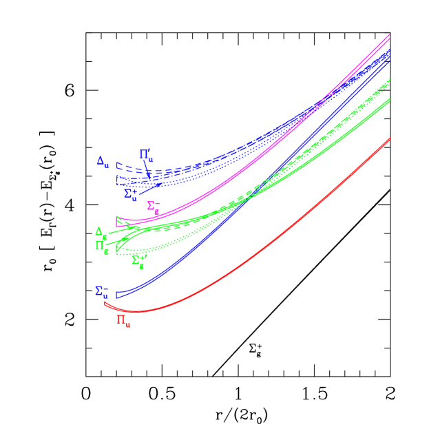
Figure 2: Continuum limit extrapolations with error range are shown for three groups of nine excited states to illustrate the prediction of the short distance operator product expansion.

should be approximately degenerate. Fig. 2 shows the excitation spectrum on a magnified scale, and it includes some of the additional states not displayed in Fig. 1 to illustrate the approximate working of the predicted degeneracies. Continuum limit extrapolations with error range are shown for three groups of nine excited states: ($\Sigma^{+}_{u},\Pi^{{}^{\prime}}_{u},\Delta_{u}$), ($\Sigma^{-}_{g},\Delta_{g},\Sigma^{+^{\prime}}_{g},\Pi_{g})$, and ($\Sigma^{-}_{u},\Pi_{u}$). Primes designate “radial” excitations in the appropriate quantum number combinations. The groups are predicted to be approximately degenerate in the multipole expansion.[4, 7] This is based on the plausible physical picture that the confined static field of the ${\rm Q\overline{Q}}$ pair is mostly dipole for ${\rm r\leq 0.3~{}fm}$ with the lowest terms dominating in the operator product expansion.

Within each group one has different string quantum numbers mixed together. For example, $\Sigma^{-}_{u}$ is N=3 and $\Pi_{u}$ is N=1, therefore the two states are expected to split into separate string levels for large r. Also, the $\Delta_{g},\Sigma^{+^{\prime}}_{g},\Pi_{g}$ states should be degenerate and sandwiched between the $\Pi_{u}$ state and the $\Sigma^{-}_{u}$ state in the string limit, with equidistant spacing in-between. Instead, they are located higher than the $\Sigma^{-}_{u}$ state at short distances, and become degenerate with the $\Sigma^{-}_{g}$ state which is an N=4 string excitation! On the intermediate scale for ${\rm 0.5~{}fm\leq r\leq 2~{}fm}$, a remarkably rapid rearrangement of the energy levels is observed.

We should also note that for r above 0.5 fm, all of the excitations shown in Fig. 1 are stable with respect to glueball decay. As r decreases below 0.5 fm, some of the excited levels eventually become unstable resonances as their energy gaps above the ground state $\Sigma_{g}^{+}$ exceed the mass of the lightest glueball. They require more care in their interpretation.

3.2 Transition Region for $0.5~{}fm\leq r\leq 2~{}fm$

One of the striking features of the transition region is the dramatic linearly-rising behavior of the $\Sigma_{\rm g}^{+}$ ground state energy in Fig. 1 once ${\rm r}$ exceeds about ${\rm 0.5~{}fm}$. The empirical function ${\rm E}_{\Sigma_{\rm g}^{+}}({\rm r})=-{\rm c}/{\rm r}+\sigma{\rm r}$ approximates the ground state energy very well for ${\rm r}\geq{\rm 0.1~{}fm}$ with the fitted constant ${\rm c=0.3}$. Early indoctrination on the popular string interpretation of the confined flux for ${\rm r}\leq{\rm 1~{}fm}$ was mostly based on the observed shape of the $\Sigma_{\rm g}^{+}$ ground state energy and some rudimentary determination of a few excited states.[11] The linear shape of the ground state potential for ${\rm r}\geq~{}{\rm 0.5~{}fm}$ and the approximate agreement of the curvature shape for ${\rm r}\leq 0.5~{}{\rm fm}$ with the ground state Casimir energy $-\pi/(12{\rm r})$ of a long confined flux[12] was interpreted as evidence for string formation. Our observed excitation spectrum clearly contradicts claims on the simple string interpretation of the linearly rising confining potential for ${\rm r\leq 2~{}fm}$. The observed energy levels, even their qualitative ordering, are in gross disagreement with expectations from a fluctuating string for quark-antiquark separations ${\rm r\leq 2~{}fm}$.

There is no solid theory for this transition region which is perhaps the most difficult to describe. It is interesting to note, however, that the somewhat phenomenological bag model does quite well in this transition region,[4] which remains the most model dependent scale with unknown microscopic details of the confinement mechanism in the QCD vacuum.

3.3 String Limit Between $2~{}fm\leq r\leq 4~{}fm$?

Although the transition region is not string-like, the rapid rearrangement of the energy levels to reach string-like level ordering around ${\rm r\approx 2~{}fm}$ is remarkable. For example, the states $\Sigma^{-}_{u}$ and $\Sigma^{-}_{g}$ break away from their respective short distance degeneracies to approach approximate string level ordering for ${\rm r\geq 2~{}fm}$ separation. In general, when we reach ${\rm r\approx 2~{}fm}$ quark-antiquark separation, after a rapid movement of the energy levels, a new level ordering emerges which qualitatively begins to resemble a naive string-like spectrum which is anticipated on quite general grounds. However, this new level ordering exhibits a finite structure whose origin is puzzling and important to understand.

A very robust feature of the effective low-energy description of a fluctuating flux sheet, or interface, in continuum euclidean space is the expected presence of massless Goldstone excitations associated with the spontaneously-broken transverse translational symmetry. The emergence of a QCD string theory from other theoretical considerations would also suggest a massless excitation spectrum. These transverse modes have energy separations above the ground state given by multiples of ${\rm\pi/r}$ for fixed ends. After the rapid transition, the level orderings and approximate degeneracies of the gluon energies at large r match, without exception, those expected of the Goldstone modes. However, the precise separation $\pi/{\rm r}$ of the energy levels is not observed in our spectrum. Some of the expected degeneracies are also significantly broken. This is likely to come from the finite size scaling theory of the underlying effective string theory which is governed by the higher dimensional operators of the effective string Lagrangian and their effects on the spectrum. In that sense the fine structure of our spectrum contains the information about the underlying effective string theory. These remarks will be illustrated in model examples of sections 4 and 5.

3.4 D=3 and D=4 SU(2) Results

The approximate string-like ordering of the energy levels between ${\rm 2~{}fm\leq r\leq 4~{}fm}$ and yet the substantial deviations from the expected locations of the massless excitations is tantalizing. Although we are beginning to understand that the complex patterns should emerge from the finite size scaling analysis of massless excitations (model examples will be given in the next section), checks on the methodology of the simulation results is important. This reason alone would motivate the tests where the original D=4, SU(3) runs were repeated with SU(2) color group in D=3 and D=4 dimensions. The D=3 SU(2) simulations have further significance. The high accuracy of the results allows more detailed comparisons with theoretical ideas which are derived from detailed studies of three-dimensional SOS models and gauge models. The fluctuating Wilson surface of the D=3 SU(2) simulations is expected to share some common features with interfaces of more simple three-dimensions gauge and spin models.

We turn now to the salient features of our SU(2) test results.

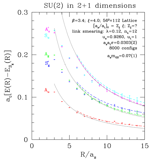
Figure 3: The energy gaps above the ground state are shown for SU(2) in D=3 dimensions. The symbols here refer to the point group representations of the surface states. The dotted lines are the expected locations of the massless Goldstone excitations. The dashed lines are ad hoc fits of the data to massive string excitations which is further discussed in the text.

The most striking feature of the D=3 and D=4 SU(2) simulations (D=3 depicted in Fig. 3) is the universality of the results:

(a)

The level orderings and approximate degeneracies of the gluon energies at large r match, without exception, those expected of the string modes for both gauge groups SU(2) and SU(3) and for D=3, or D=4.

(b)

Even the fine structure of the split spectrum shows a great deal of universality in the character of its substantial deviations from the expected massless spectrum at large separations. First, in D=4 dimensions we observed that the deviations in the string formation region ${\rm 2~{}fm\leq r\leq 4~{}fm}$ can be roughly described by replacing the expected massless excitation spectrum with an ad hoc fit to massive surface excitations parametrized by a new scale parameter ${\rm m_{s}}$. Although the numerical value of ${\rm m_{s}}$ varies somewhat in the three cases we considered, this replacement alone describes qualitatively the splitting patterns which occur in all simulations for string quantum numbers which otherwise should be degenerate. The significance of the apparent mass term is unclear. Very likely, it is only an artificial description of finite size power corrections to the massless string spectrum. More work is needed to clarify this, because a massive QCD string is not an entirely excluded possibility.

(c)

One more important test was done in our simulations. We rotated out the static quark-antiquark pair from the main axis of the lattice and determined the spectrum again in the diagonal off-axis position. All the spectra we determined remained the same within error bars. This is significant for later discussions. It supports the the plausible argument that we are sitting in the rough phase of the large Wilson surface at the values of the coupling constants where our extensive simulation results were obtained.

3.5 Strong Coupling Tests

To make sure that the rather sophisticated lattice technology we applied is working we determined the excitation spectrum in extensive test runs at strong coupling in three-dimensional SU(2). This gave us the opportunity to compare analytic results with our lattice technology. We calculated the string spectrum in leading nontrivial order for r=3a and r=4a separations of the static sources, on axis, at very strong coupling where the next to leading correction is expected to be in the percent range. Fig. 4

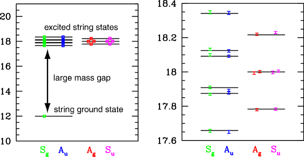
Figure 4: Strong coupling tests of massive “string” excitations for D=3 in SU(2). The solid lines are calculated analytically and the simulation results for 20 states sit within errors. The large energies required huge lattice aspect ratios which is the most challenging part of our lattice technology. The scale is set by the lattice spacing a.

displays the simulation results and the analytic predictions which are in excellent agreement. This is a very nontrivial test supporting our belief that the peculiar fine structure of our results in the string formation region of ${\rm 2~{}fm\leq r\leq 4~{}fm}$ is not an artifact of the simulation method which performs so well under very difficult conditions.

4 Surface Excitation Spectrum in Z(2) Spin and Gauge Models

One of our extensive tests above included a detailed study of the Wilson surface excitation spectrum of the D=3 SU(2) gauge model of ${\rm QCD_{3}}$. The Abelian subgroup Z(2) of SU(2) is expected to play an important role in the microscopic mechanisms of quark confinement suggesting that Wilson surface physics of the D=3 Z(2) gauge spin model should have qualitative and quantitative similarities with the theoretically more difficult ${\rm QCD_{3}}$ case. In the critical region of the Z(2) model we have a rather reasonable description of continuum string formation based on the excitation spectrum of a semiclassical defect line (soliton) of the equivalent ${\rm\Phi^{4}}$ field theory. This is the analogue of the effective Landau-Ginzburg equations of QCD. It is useful to investigate surface physics in the BCSOS model, first. The surface physics of the Z(2) gauge model is closely related to the BCSOS model by universality argument and a duality transformation.

4.1 Interface Spectrum in the BCSOS Model

This model was proposed by Beijeren[14] as the simplest interface which can be investigated by analytic methods. We start from a body-centered cubic Ising model with ferromagnetic nearest neighbor coupling J’ (between sites at the center and on the corner of an elementary cube as illustrated in Fig. 5). The next-nearest-neighbor coupling J is defined

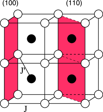
Figure 5: The two couplings J and J’ of the BC Ising lattice are defined in the text.

along the three main lattice directions. An interface can be created in the horizontal direction by keeping the spins in the two bottom layers positive and those in the two top layers negative. Free, or periodic boundary conditions can be imposed on the side walls of the finite three-dimensional lattice. The body-centered solid-on-solid (BCSOS) model is obtained by letting J’ approach infinity and keeping J constant. The SOS condition is satisfied in this limit and the fluctuating interface, with a height measured from a horizontal base, separates the negative spin phase from the positive one. For roughening studies, the BCSOS limit is expected to differ from the symmetric J=J’ BC Ising model only by a few percent, since only very few wrong phase bubbles exist in the bulk around the roughening transition of the fluctuating interface.

The BCSOS model can be mapped into the six-vertex model for which the Bethe Ansatz equations are known.[15] Beijeren showed from the Bethe Ansatz that the BCSOS model has a phase transition at ${\rm T_{R}=J/(k_{B}\cdot 2ln2)}$ which is identified as the critical temperature of the roughening transition of the interface. For ${\rm T<T_{R}}$ the interface is smooth with a finite mass gap in its excitation spectrum. For ${\rm T\geq T_{R}}$ the mass gap vanishes and the interface exhibits a massless excitation spectrum. The roughening transition is of the Kosterlitz-Thouless type in the model.

The connection with the Z(2) gauge model is rather straightforward. The simple cubic Ising model is in the same universality class as the body-centered Ising model. It follows then that the SOS limit of the simple cubic Ising model should be very similar to the BCSOS model. In fact, we expect that the low energy spectra of the two interfaces should exactly map into each other, after appropriate rescaling of the temperatures. In addition, we expect the SOS limits of both models to differ only by a few percent from the interfaces of the original models. Therefore the BCSOS interface should behave essentially the same as the interface of the simple cubic Ising model. As the final step of the transformation, we note that the simple cubic Ising model can be mapped by a duality transformation into the D=3 Z(2) gauge model on a simple cubic lattice. This is the wanted result: the spectrum of the BCSOS interface should be the same as the spectrum of the Wilson surface in the Z(2) gauge model.

Since we are interested in the full excitation spectrum of the Wilson surface, we determined the low energy part of the full spectrum from direct diagonalization of the transfer matrix of the BCSOS model. A periodic boundary condition was used, which corresponds to the spectrum of a periodic Polyakov line in the Z(2) gauge model. With a flux of period L we used exact diagonalization for ${\rm L\leq 16}$, and the the Bethe Ansatz equations up to L=1024. The direct diagonalization was mainly used for checks and establishing the pattern of level ordering. The following picture emerges from the calculation for large L values in the massless Kosterlitz-Thouless (KT) phase. The ground state energy of the flux is given by

$${\rm E_{0}(L)=\sigma_{\infty}\cdot L-\frac{\pi}{6L}c+o(1/L)~{},}$$ (4)

where $\sigma_{\infty}$ is the string tension, c designates the conformal charge, which is found to be c=1 to very high accuracy, consistent with the fact that we are in the KT phase. The o(1/L) term designates the corrections to the leading 1/L behavior; they decay faster than 1/L. At the critical point of the roughening transition, the corrections can decay very slowly, like ${\rm 1/(lnL\cdot L)}$. Away from the critical point, the corrections decay faster than 1/L in power-like fashion with some logarithmic corrections.

For each operator ${\rm O_{\alpha}}$ which creates states from the vacuum with quantum numbers $\alpha$, there is a tower excitation spectrum above the ground state,

$${\rm E^{\alpha}_{j,j^{\prime}}(L)=E_{0}(L)+\frac{2\pi}{L}(x_{\alpha}+j+j^{\prime})+o(1/L)~{},}$$ (5)

where the nonnegative integers j,j’ label the conformal tower and ${\rm x_{\alpha}}$ is the anomalous dimension of the operator ${\rm O_{\alpha}}$. The momentum of each excitation is given by

$${\rm P^{\alpha}_{j,j^{\prime}}(L)=\frac{2\pi}{L}(s_{\alpha}+j-j^{\prime})~{},}$$ (6)

where ${\rm s_{\alpha}}$ is the spin of the operator ${\rm O_{\alpha}}$.

The surface excitation spectrum described by Eqs. (4, 5, 6) is not a simple massless string spectrum with obvious geometric interpretation. There are excitations with noninteger values of the anomalous dimensions ${\rm x_{\alpha}}$ which continuously vary with the Ising coupling J. In fact, we found an infinite sequence of operators which excite surface states with fractional multiples of ${\rm 2\pi/L}$, instead of integer multiples of ${\rm 2\pi/L}$, as expected in a naive string picture. This sequence can be labelled by anomalous dimensions

$${\rm x^{G}_{n,m}=\frac{n^{2}}{4\pi K}+\pi Km^{2}~{},}$$ (7)

where n,m are nonnegative integers and the constant K depends in a known way on the BCSOS coupling constant J. The physical interpretation of the rather peculiar excitations of the rough gapless surface will be discussed elsewhere. Here it is sufficient to note that the spectrum is related to a free compactified Gaussian field, but the field configuration allow for line defects, presumably related to dislocations of the fluctuating rough surface.

4.2 Surface Physics in the Three-Dimensional Z(2) Gauge Model

First, we note that the SOS mapping of the Wilson surface close to the roughening transition is not sensitive to the group structure of the particular model in D=3 dimensions. It is known that the SOS mapping in the Z(2) gauge model is accurate to a few percent around the roughening transition. Assuming that the same is true in the SU(2) ${\rm QCD_{3}}$ model, we should expect very similar surface roughening behavior in the two models after an appropriate rescaling of the gauge couplings into the effective coupling constant of the SOS model.

A great deal more is known about the Z(2) gauge model in D=3 dimensions. Our goal is to draw analogy between the Z(2) model and the behavior of ${\rm QCD_{3}}$ with SU(2) color which happens to exhibit most of the salient features of all the other QCD simulations in the string formation region. The phase diagram in the bulk and its Wilson surface physics are summarized in Fig. 6. Based on the above remarks, we expect that the analogy between SU(2) ${\rm QCD_{3}}$ and Z(2) remains useful throughout the entire gapless rough phase of the Wilson surface, from the roughening transition to continuum string formation.

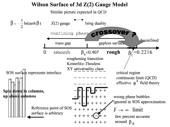
Figure 6: The phase diagram of the bulk in the Z(2) gauge model and the most important features of its Wilson surface are summarized here. The horizontal axis represents ${\rm 1/\beta}$ on some arbitrary scale. The zero temperature limit of the Ising representation corresponds to ${\rm 1/\beta=0}$ on the left end which is the strong coupling limit of the Z(2) gauge model representation. Wrong phase bubbles are ignored in the SOS representation of the surface which separates the spin-up region from the spin-down region in Ising respresentation. These bubbles are eliminated and the SOS approximation becomes exact in the ${\rm J^{\prime}\rightarrow\infty}$ limit of the vertical Ising coupling.

The key to the understanding of the phase diagram is the well-known fact that the D=3 Z(2) gauge model is dual to the D=3 Ising spin model. For the inverse gauge coupling $\overline{\beta}$ of the Z(2) model the dual mapping onto ${\rm\beta=1/kT}$ of the Ising model is given in Fig. 6. In the bulk, the Z(2) model has a confining phase which corresponds to the ordered phase of the Ising representation. This confined phase ends at the bulk critical point ${\rm\beta_{c}=0.2216}$. In drawing analogy with the SU(2) ${\rm QCD_{3}}$ model, we should consider the confined phase of the Z(2) model only. The ${\rm 1/\beta=0}$ point on the left of the phase diagram maps into the ${\rm g\rightarrow\infty}$ strong coupling limit of ${\rm QCD_{3}}$ whereas the ${\rm\beta_{c}=0.2216}$ Ising critical point of the bulk maps into the ${\rm g\rightarrow 0}$ continuum limit of ${\rm QCD_{3}}$.

The roughening transition region:
The confining flux sheet of the Wilson loop in the Z(2) gauge model corresponds to the Ising interface in the dual representation. The on-axis Z(2) Wilson surface exhibits a roughening transition at ${\rm g_{R}}$ which maps into the inverse roughening temperature ${\rm\beta_{R}=0.407}$ of the Ising interface. At the roughening point, the bulk is far from the critical coupling ${\rm g_{c}}$ of the Z(2) model which maps into the critical coupling ${\rm\beta_{c}=0.2216}$ of the Ising representation. This should correspond to the g=0 continuum limit in ${\rm QCD_{3}}$. The surface excitation spectrum in the roughening region exhibits a surprisingly rich spectrum which is difficult to interpret as an effective string theory based on a simple geometric picture of the fluctuating interface. Some details of the spectrum were outlined earlier in this section for the BCSOS representation where we presented the exact solution. The two spectra should be essentially identical by universality arguments. The continuum limit in the bulk:
When we move with the gauge coupling into the critical region, depicted in Fig. 6 as the close neighborhood of ${\rm\beta_{c}=0.2216}$ on the left, the SOS aproximation is not valid anymore due to large fluctuations in the bulk. A complementary description is expected to work in this region in terms of a renormalization group improved semiclassical expansion of the effective ${\rm\Phi^{4}}$ field theory, describing the critical region of the Z(2) model in Ising representation. The Wilson surface is described by a classical soliton solution of the $\Phi^{4}$ field equations. Excitations of the surface are given by the spectrum of the fluctuation operator

$${\mathcal{M}}=-\nabla^{2}+{\rm U}^{\prime\prime}(\Phi_{\rm soliton})$$ (8)

where ${\rm U(\Phi)}$ is the field potential energy of the $\Phi^{4}$ field. The spectrum of the fluctuation operator ${\mathcal{M}}$ of the finite surface is determined from a two-dimensional Schrödinger equation with a potential of finite extent[13]. An example is shown in Fig. 7 for L=30 separation of the two fixed ends of the clamped Wilson surface at correlation length ${\rm\xi=1.87}$ in the bulk.

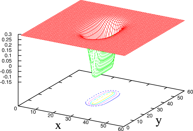
Figure 7: The effective potential of the Schrödinger equation.

In the limit of asymptotically large surfaces, the equation becomes separable in the longitudinal and transverse coordinates. The transverse part of the spectrum is in close analogy with the quantization of the one-dimensional classical $\Phi^{4}$ soliton. There is always a discrete zero mode in the spectrum which is enforced by translational invariance in the transverse direction. The surface excitations have the form ${\rm\Psi(x)\cdot exp(iqy),~{}q=\pi n/L,~{}n=1,2,3...}$, where the wavefuncion ${\rm\Psi(x)}$ represents the soliton zero mode. In Fig. 8 we compare the second string state from the semiclassical expansion with our direct simulation results.

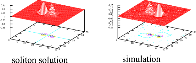
Figure 8: The string soliton configuration corresponds to L=20 with clamped ends and bulk correlation length ${\rm\xi=1.87}$.

In agreement with the semiclassical string soliton picture, we find a very accurate string spectrum even for correlation lengths ${\rm\xi\leq 1}$ as shown in Fig. 9.

Figure 9: The string spectrum of the Z(2) model is calculated here for a location half way between the roughening transition and bulk criticality.

The zero mode of the soliton is distorted on the lattice due to the explicit breaking of translational invariance. In the leading semiclassical expansion this will generate a gap which is the analogue of the Peierls-Nabarro gap in lattice soliton physics. This gap is very significant for small correlation lengths, as depicted in Fig. 10.

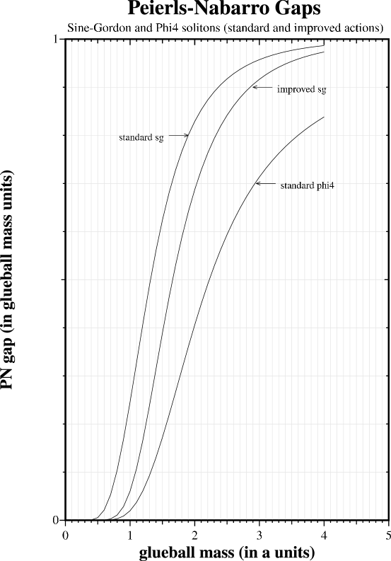
Figure 10: Peierls-Nabarro gap in the string spectrum for various scalar field theories in D=3 dimensions. The glueball mass is defined as the inverse correlation length in the bulk.

There is no trace of this gap in our simulations in Fig. 9. The best guess is that tunneling and fluctuation effects, as the string soliton moves in the periodic lattice potential, destroy the effect.

5 What Is the Continuum Limit of QCD String Theory?

Large Wilson loops in QCD represent the euclidean time evolution of the gluon field generated by the static quark-antiquark pair at large separation. It is generally assumed that some confining flux develops and the physical interpretation of its excitation spectrum in lattice QCD requires a detailed understanding of critical phenomena on large Wilson surfaces. In this section, we first outline our understanding of the roughening transition of the Wilson surface in lattice QCD and the crossover in surface criticality as we approach the continuum limit in the bulk. This is mostly based on our study of the Z(2) gauge model and the BCSOS model as presented earlier.

5.1 What is the String Interpretation of Roughening?

If the $Q\overline{Q}$ pair is located along one of the principal axes on the lattice in some spatial direction, the Wilson surface at strong coupling becomes smooth in technical terms. This implies the existence of a mass gap in its excitation spectrum, as seen for example in the strong coupling tests of our simulation technology, displayed in Fig. 4. The mass gap is responsible for suppressing the fluctuations of the Wilson surface away from its minimal area in the plane as determined by two principal lattice axes. One of the axes represents the space-like connection between the static color sources and the other axis designates euclidean time. From the viewpoint of statistical physics, the two directions are equivalent, and we can talk about surface physics and its excitation spectrum without further reference to the original physical picture of the confined quark-antiquark pair and its gluon excitation spectrum.

As the coupling weakens, a roughening transition is expected in the surface at some finite gauge coupling ${\rm g=g_{R}}$ where the gap in the excitation spectrum vanishes. The correlation length in the surface diverges at the critical point ${\rm g_{R}}$ of the roughening transition and it is expected to remain infinite for any value of the gauge coupling when ${\rm g\leq g_{R}}$. At the roughening transition, the bulk behavior remains far separated from the critical region of the continuum theory which is located in the vicinity of ${\rm g=0}$. Technically, this implies that the surface will exhibit an infinite surface correlation length (rough surface) while the bulk correlation length is of the order one. Based on strong coupling series analysis and on the approximate mapping of the Wilson surface fluctuations into the solid on solid interface model, surface roughening with the collapse of the mass gap at ${\rm g=g_{R}}$ is expected to show the characteristics of the Kosterlitz-Thouless phase transition.

The low energy excitation spectrum of the Wilson surface for ${\rm g\leq g_{R}}$ and not far from ${\rm g_{R}}$, in the domain of the critical KT phase, should be essentially identical to Eqs. (4, 5, 6) of our BCSOS spectrum in ${\rm QCD_{3}}$. This spectrum exhibits the features of a two-dimensional conformal field theory with c=1 conformal charge. In ${\rm QCD_{4}}$ we do not expect qualitative changes. The precise physical interpretation of the spectrum around the roughening point in terms of a geometric string theory will require further work. This is facilitated by the observation that the spectrum is equivalent to that of the two-dimensional Gaussian scalar field on a circle, including defect lines in the field configurations of the path integral for the partition function.

5.2 Crossover to continuum QCD

Now, is the Kosterlitz-Thouless picture identical to what we expect in continuum ${\rm QCD_{3}}$ string theory? As we have seen, the Wilson surface in ${\rm QCD_{3}}$ is in the massless Kosterlitz-Thouless phase for gauge couplings weaker than the roughening coupling. Based on universality arguments, this alone should determine the complete low-energy spectrum of the surface. However, as the coupling weakens below ${\rm g_{R}}$ and we take the ${\rm g\rightarrow 0}$ continuum limit, an important question arises. Do we expect a change in the structure of the low energy spectrum from the KT universality class into something else which should be identified as the universality class of continuum QCD string theory? This transition from the KT phase to continuum ${\rm QCD_{3}}$ string theory should be particularly intriguing. On one hand, the expected transition is quite plausible, given the fact that we are sitting at ${\rm g_{R}}$ in the bulk which is far from the critical region of the continuum limit. Why would this rough surface look identical to the continuum Wilson surface? On the other hand, the Wilson surface is unlikely to go back into a massive phase again as we move towards ${\rm g=0}$. This would require a new critical point ${\rm g_{c}}$ somewhere between ${\rm g_{R}<g_{c}<0}$ which is not likely. The only plausible scenario is that the surface remains massless throughout the ${\rm g_{R}\leq g\leq 0}$ region and its critical behavior will cross over from the Kosterlitz-Thouless class into the universality class of continuum QCD string theory whose precise description remains the subject of our future investigations.

Appendix

Three exact quantum numbers which are based on the symmetries of the problem determine the classification scheme of the gluon excitation spectrum. We adopt the standard notation from the physics of diatomic molecules and use $\Lambda$ to denote the magnitude of the eigenvalue of the projection $\vec{J_{g}}\!\cdot\hat{\bf r}$ of the total angular momentum $\vec{J_{g}}$ of the gluon field onto the molecular axis $\hat{\bf r}$. The capital Greek letters $\Sigma,\Pi,\Delta,\Phi,\dots$ are used to indicate states with $\Lambda=0,1,2,3,\dots$, respectively. The combined operations of charge conjugation and spatial inversion about the midpoint between the quark and the antiquark is also a symmetry and its eigenvalue is denoted by $\eta_{CP}$. States with $\eta_{CP}=1(-1)$ are denoted by the subscripts $g$ ($u$). There is an additional label for the $\Sigma$ states; $\Sigma$ states which are even (odd) under a reflection in a plane containing the molecular axis are denoted by a superscript $+$ $(-)$. Hence, the low-lying levels are labelled $\Sigma_{g}^{+}$, $\Sigma_{g}^{-}$, $\Sigma_{u}^{+}$, $\Sigma_{u}^{-}$, $\Pi_{g}$, $\Pi_{u}$, $\Delta_{g}$, $\Delta_{u}$, and so on. For convenience, we use $\Gamma$ to denote these labels in general.

The gluon excitation energies $E_{\Gamma}(\vec{r})$ were extracted from Monte Carlo estimates of generalized large Wilson loops. Recall that the well-known static potential $E_{\Sigma_{g}^{+}}(r)$ can be obtained from the large-$t$ behaviour $\exp[-tE_{\Sigma_{g}^{+}}(r)]$ of the Wilson loop for a rectangle of spatial length $r$ and temporal extent $t$. In order to determine the lowest energy in the $\Gamma$ sector, each of the two spatial segments of the $r\times t$ rectangular Wilson loop must be replaced by a sum of spatial paths, all sharing the same starting and terminating sites, which transforms as $\Gamma$ under all symmetry operations. The easiest way to do this is to start with a single path ${\cal P}_{\alpha}$, such as a staple, and apply the $\Gamma$ projection operator which is a weighted sum over all symmetry operations; this yields a single gluon operator in the $\Gamma$ channel. Different gluon operators correspond to different starting paths ${\cal P}_{\alpha}$. Using several (in some channels as many as 40) different such operators then produces a matrix of Wilson loop correlators $W_{\Gamma}^{ij}(r,t)$.

Monte Carlo estimates of the $W_{\Gamma}^{ij}(r,t)$ matrices were obtained in several simulations performed on our Beowolf class UP2000 Alpha cluster using an improved gauge-field action[9]. The couplings $\beta$, input aspect ratios $\xi$, and lattice sizes for each simulation will be listed in tables of our forthcoming publication[6]. Our use of anisotropic lattices in which the temporal lattice spacing $a_{t}$ was much smaller than the spatial spacing $a_{s}$ was crucial for resolving the gluon excitation spectrum, particularly for large $r$. The couplings in the action depend not only on the QCD coupling $\beta$, but also on two other parameters: the mean temporal link $u_{t}$ and the mean spatial link $u_{s}$. Following earlier work[9], we set $u_{t}=1$ and obtain $u_{s}$ from the spatial plaquette. We correct $a_{s}/a_{t}=\xi$, the input or bare anisotropy, in all of our calculations, by determining the small radiative corrections to the anisotropy as finite lattice spacing corrections which vanish in the continuum limit.

To hasten the onset of asymptotic behaviour, iteratively-smeared spatial links[9] were used in the generalized Wilson loops. A single-link procedure was used in which each spatial link variable $U_{j}(x)$ on the lattice is mapped into itself plus a sum of its four neighbouring (spatial) staples multiplied by a weighting factor $\zeta$. The resulting matrix is then projected back into SU(3). This mapping is then applied recursively $n_{\zeta}$ times, forming new smeared links out of the previously-obtained smeared links. Separate measurements were taken for each smearing; cross correlations were not determined. The temporal segments in the Wilson loops were constructed from thermally-averaged links, whenever possible, to reduce statistical noise.

References

- [1] K.J. Juge, J. Kuti, and C. Morningstar, \JournalNucl. Phys. B (Proc. Sup.)633261998.
- [2] K.J. Juge, J. Kuti, and C. Morningstar, \JournalNucl. Phys. B (Proc. Sup.)735901999.
- [3] Work in progress.
- [4] K.J. Juge, J. Kuti, and C. Morningstar, \JournalNucl. Phys. B (Proc. Sup.)635431999.
- [5] J. Kuti, Internal report.
- [6] K.J. Juge, J. Kuti, and C. Morningstar, In preparation.
- [7] N. Brambila, A. Pineda, J. Soto, and A. Vairo, \JournalNPB5662752000.
- [8] R. Sommer, \Journal\NPB4118391994.
- [9] C. Morningstar and M. Peardon, \Journal\PRD5640431997.
- [10] M. Peter, \Journal\NPB5014711997.
- [11] S. Perantonis and C. Michael, \Journal\NPB3478541990.
- [12] M. Lüscher, \Journal\NPB1803171981.
- [13] J. Kuti, \JournalNucl. Phys. B (Proc. Sup.)73721999.
- [14] H. van Beijeren, \Journal\PRL389931977.
- [15] E.H. Lieb, \Journal\PRL1810641967.