Photon Structure Functions from Quenched Lattice QCD

Abstract

We calculate the first moment of the photon structure function, $\langle x\rangle^{\gamma}=\int^{1}_{0}dxF^{\gamma}_{2}(x,Q^{2})$, on the quenched lattices with $\beta=6.0$ using the formalism developed by the authors recently. In this exploratory study, we take into account only the connected contractions. The result is compared with the experimental data as well as model predictions.

The parton (quark and gluon) distributions in hadrons, which can be measured from lepton-hadron deep inelastic scattering and other hard processes, have played a crucial role in understanding high-energy scattering and the hadron structure. Recently it has become possible to calculate moments of these distributions from first principles using lattice QCD [1, 2, 3].

There are many other physical observables which are yet to be calculated from lattice QCD. A special class of of these involve either virtual or real photons. Until recently, the conditions under which these quantities can be calculated using lattice QCD remained unclear. The reason is that the photon is not an eigenstate of QCD. Rather, a “photon” state in nature is a superposition of the U(1) gauge boson and quark-gluon configurations which are suppressed by the electromagnetic coupling. The matrix elements of QCD operators in the photon states are time-dependent correlations which are defined in the Minkowski space, and the standard method used for calculating hadron matrix elements on the lattice is not directly applicable [1, 2, 3].

In our earlier paper [4], we showed that the matrix element of a quark-gluon operator between photon states can be evaluated using lattice QCD. The relevant expression is

$$\langle\gamma(p\lambda^{\prime})|{\cal O}(0)|\gamma(p\lambda)\rangle=-e^{2}\int d^{4}xd^{4}ye^{\omega(x_{4}-y_{4})}e^{-i\vec{p}\cdot(\vec{x}-\vec{y})}\langle 0|T_{E}\epsilon^{*}(\lambda^{\prime})\cdot J(x){\cal O}(0)\epsilon(\lambda)\cdot J(y)|0\rangle$$ (1)

where every quantity has been expressed in the Euclidean space: $T_{E}$ is the Euclidean time-ordering; the electromagnetic current $J_{\mu}(\mu=1,2,3,4)$ is defined as $\sum_{f}e_{f}\overline{\psi}_{f}\gamma_{\mu}\psi_{f}$ with Euclidean $\gamma$ matrices $\gamma_{i}=-i\gamma_{M}^{i}(i=1,2,3)$ and $\gamma_{4}=\gamma^{0}$; the Euclidean photon polarization vector is defined as $\epsilon_{i}=\epsilon^{i}_{M}$ and $\epsilon_{4}=i\epsilon^{0}(\epsilon^{*4}=i\epsilon^{*0})$; $i\omega$ is the Euclidean-space photon energy. [In Ref. [4], we did not continue the electromagnetic current and the polarization vector to Euclidean space and superficially the result there differs by an overall sign.] The above expression is the same as the naive analytic continuation of the matrix element from the Minkowski space. However, Eq. (1) is only valid when there exists an energy gap between the photon energy and the lowest hadronic state of the same quantum number. Otherwise, the integral becomes divergent.

One of the quantities we can study using the above formalism is the photon structure functions, which can be measured from collisions between real or virtual photons with highly virtual ones, achievable in $e^{+}e^{-}\rightarrow e^{+}e^{-}+$hadrons [5, 6]. While a photon is normally considered a structureless particle, it can fluctuate into a charged fermion-antifermion pair or more complicated hadronic states which can be revealed through interactions with a highly virtual photon. In fact, the photon structure functions can be defined from its hadronic tensor and the moments of the structure functions can be obtained from operator product expansion, much in the same way as for the hadron structure functions. There exists a substantial amount of experimental data for unpolarized structure functions already [6]; and future experiments from HERA and $e^{+}e^{-}$ are expected to measure the polarized structure functions as well [7]. (For a recent review on theoretical and experimental progress on this subject, refer to Ref. [6].)

Here we report on the first lattice study of the structure function $F^{\gamma}_{2}$. More specifically, we measure the first moment of $F_{2}^{\gamma}$ which corresponds to the average fractional momentum carried by the quarks (weighed with the fractional charge squared for each flavor) in a real photon. The measurement is done on $\beta=6.0$ lattices, corresponding to $Q^{2}\sim a^{-2}\sim(2.4~{}\mbox{GeV})^{2}$, in the quenched approximation for three degenerate flavors of quarks. Also, we choose to ignore the contributions from disconnected diagrams in which the quark lines do not connect any of the external vertices.

We begin by briefly reviewing the definition of the photon structure functions and their relation to the cross sections. We closely follow [8] for the definition of $F^{\gamma}_{2}(x,Q^{2})$. For the deep inelastic $e+\gamma$ process in a frame where the incoming electron and the photon are collinear, we write

$$e^{\pm}(k)+\gamma(p)\rightarrow e^{\pm}(k^{\prime})+X(p_{X})\ ,$$ (2)

$$k^{\mu}=(E,0,0,E)\ ,$$ (3)

$${k^{\prime}}^{\mu}=(E^{\prime},0,E^{\prime}\sin\theta,E^{\prime}\cos\theta)\ ,$$ (4)

$$p^{\mu}=(E_{\gamma},0,0,-E_{\gamma})\ .$$ (5)

The relevant kinetic variables are $Q^{2}=-(k-k^{\prime})^{2}$, $\nu=p\cdot q$, $q=k-k^{\prime}$, $x=Q^{2}/2(p\cdot q)$, $y=q\cdot p/k\cdot p$. The photon structural information is contained in the following tensor,

$$W^{\mu\nu} = \frac{1}{4\pi}\cdot\frac{1}{2}\sum_{X,\lambda}\langle\gamma(p\lambda)|J^{\mu}(0)|X\rangle\langle X|J^{\nu}(0)|\gamma(p\lambda)\rangle(2\pi)^{4}\delta^{4}(p_{X}-p-q)$$ (6)

$$= \frac{1}{4\pi}\cdot\frac{1}{2}\sum_{\lambda}\int\langle\gamma(p\lambda)|[J^{\mu}(x),J^{\nu}(0)]|\gamma(p\lambda)\rangle e^{iqx}d^{4}x$$ (7)

$$= W^{\gamma}_{1}(\nu,Q^{2})\left[-g^{\mu\nu}+\frac{q^{\mu}q^{\nu}}{q^{2}}\right]+W^{\gamma}_{2}(\nu,Q^{2})\left[p^{\mu}-\frac{p\cdot q}{q^{2}}q^{\mu}\right]\left[p^{\nu}-\frac{p\cdot q}{q^{2}}q^{\nu}\right].$$ (8)

Here $J_{\mu}(x)=\sum_{f}e_{f}\overline{\psi}_{f}(x)\gamma_{\mu}\psi_{f}(x)$ is the electromagnetic current and $e_{f}$ is the fractional charge of the quark of flavor $f$. The covariant normalization has been used for the photon state, $\langle\gamma(p\lambda)|\gamma(p^{\prime}\lambda^{\prime})\rangle=(2\pi)^{3}2\omega_{\vec{p}}\delta(\vec{p}-\vec{p^{\prime}})\delta_{\lambda,\lambda^{\prime}}$.

Since we are interested in the unpolarized photon properties here, we have averaged over the photon polarization $\lambda$ in the above equations. [The polarized photon structure functions are interesting by themselves and can be studied in a similar approach [7].]

Using these variables, the differential cross section is given by

$$\frac{d\sigma}{dE^{\prime}d\cos\theta}=\frac{8\pi\alpha^{2}_{\rm em}{E^{\prime}}^{2}}{Q^{4}E_{\gamma}}\bigg{[}2E^{2}_{\gamma}W^{\gamma}_{2}(\nu,Q^{2})\cos^{2}\left(\frac{\theta}{2}\right)+W^{\gamma}_{1}(\nu,Q^{2})\sin^{2}\left(\frac{\theta}{2}\right)\bigg{]}\ ,$$ (9)

or, in terms of $x$ and $y$ and scaling functions,

$$\frac{d\sigma}{dxdy}=\frac{16\pi\alpha_{\rm em}^{2}EE_{\gamma}}{Q^{4}}\bigg{[}(1-y)F_{2}^{\gamma}(x,Q^{2})+xy^{2}F^{\gamma}_{1}(x,Q^{2})\bigg{]}\ ,$$ (10)

where the dimensionless scaling functions are defined as $F_{2}^{\gamma}(x,Q^{2})=\nu W^{\gamma}_{2}(\nu,Q^{2})$ and $F^{\gamma}_{1}(x,Q^{2})=W^{\gamma}_{1}(\nu,Q^{2})$.

In the parton model, the photon scaling function $F_{2}^{\gamma}(x)$ is related to the quark distributions $q_{f}^{\gamma}(x)$ in the photon—the probability of finding a quark with momentum fraction $x$,

$$F^{\gamma}_{2}(x)=x\cdot\sum_{f}e_{f}^{2}(q_{f}^{\gamma}(x)+\overline{q}_{f}^{\gamma}(x))\ .$$

Taking into account QCD radiative corrections, the moments of the photon structure functions can be written in the following factorized form,

$$\int^{1}_{0}x^{n-2}F_{2}^{\gamma}(x,Q^{2})\ dx=\sum_{f}C_{2n,f}\left(\frac{Q^{2}}{\mu^{2}},g(\mu)\right)\langle x^{n-1}\rangle^{\gamma}_{f}\ ,~{}~{}~{}~{}(n=2,4,...,)$$

where $C_{2n,f}$ are the perturbative coefficient functions and $\langle x^{n-1}\rangle^{\gamma}_{f}$ are the nonperturbative moments of the parton (quark and gluon) distributions ($f$ here refers to gluons as well). For quarks, the moments can be calculated as the matrix elements of local operators,

$$\frac{1}{2}\sum_{\lambda}\langle\gamma(p\lambda)|{\cal O}_{\{\mu_{1}\cdots\mu_{n}\},f}|\gamma(p\lambda)\rangle=2\langle x^{n-1}\rangle^{\gamma}_{f}[p_{\mu_{1}}\cdots p_{\mu_{n}}-{\rm traces}]\ ,$$ (11)

$${\cal O}_{\mu_{1}\cdots\mu_{n},f}=\left(\frac{i}{2}\right)^{n-1}\overline{\psi}_{f}\gamma_{\mu_{1}}\stackrel{{\scriptstyle\leftrightarrow}}{{D}}_{\mu_{2}}\cdots\stackrel{{\scriptstyle\leftrightarrow}}{{D}}_{\mu_{n}}\psi_{f}\ ,$$ (12)

where $\stackrel{{\scriptstyle\leftrightarrow}}{{D}}_{\mu}=\stackrel{{\scriptstyle\rightarrow}}{{D}}_{\mu}-\stackrel{{\scriptstyle\leftarrow}}{{D}}_{\mu}$ is the covariant derivative and $\{\cdots\}$ denotes the symmetrization of indices.

In the following discussion, we ignore the radiative corrections to the coefficient functions and take $C_{2n,f}=e_{f}^{2}$ for quarks and 0 for gluons. We then define $\langle x\rangle^{\gamma}=\int^{1}_{0}F_{2}^{\gamma}(x,Q^{2})dx$, which can be calculated as the matrix elements of the following operator;

$${\cal{O}}^{\rm(cont)}_{\mu\nu}(x)=\sum_{f}e_{f}^{2}\cdot\frac{i}{2}\overline{\psi}_{f}(x)\gamma_{\{\mu}\stackrel{{\scriptstyle\leftrightarrow}}{{D}}_{\nu\}}\psi_{f}(x)\ .$$ (13)

In lattice QCD, we need to define the corresponding lattice operator in Euclidean space:

$${\cal{O}}^{\rm(latt)}_{\mu\nu}(x)=\sum_{f,y}e_{f}^{2}~{}\left[\overline{\psi}_{f}(x)\Gamma^{\cal{O}}_{\mu\nu}(x,y)\psi_{f}(y)+\overline{\psi}_{f}(y)\Gamma^{\cal{O}}_{\mu\nu}(y,x)\psi_{f}(x)\right]\ ,$$ (14)

$$\Gamma^{\cal{O}}_{\mu\nu}(x,y)=\frac{i}{8}\left[\gamma_{\mu}(U_{\nu}(x)\delta_{y,x+\hat{\nu}}-U^{\dagger}_{\nu}(y)\delta_{y,x-\hat{\nu}})+(\mu\leftrightarrow\nu)\right]\ ,$$ (15)

where the lattice spacing($a$) is set to 1 and the lattice covariant derivatives are defined as

$$\stackrel{{\scriptstyle\rightarrow}}{{D}}_{\mu}\psi(x)=\frac{1}{2}(U_{\mu}(x)\psi(x+\hat{\mu})-U^{\dagger}_{\mu}(x-\hat{\mu})\psi(x-\hat{\mu}))\ ,$$

$$\overline{\psi}(x)\stackrel{{\scriptstyle\leftarrow}}{{D}}_{\mu}=\frac{1}{2}(\overline{\psi}(x+\hat{\mu})U^{\dagger}_{\mu}(x)-\overline{\psi}(x-\hat{\mu})U_{\mu}(x-\hat{\mu}))\ .$$

The corresponding Euclidean matrix element to Eq. (12) is

$$\frac{1}{2}\sum_{\lambda}\langle\gamma(p\lambda)|{\cal{O}}^{\rm(latt)}_{\mu\nu}|\gamma(p\lambda)\rangle=2i\langle x\rangle^{\gamma}p_{\mu E}p_{\nu E}\ ,$$ (16)

where the photon Euclidean four-momentum is defined as $p_{\mu E}=(\vec{p},i\omega)$.

The photon matrix element in lattice QCD is

$$\langle\gamma(p\lambda^{\prime})|{\cal O}_{\mu\nu}(0)|\gamma(p\lambda)\rangle^{\rm(latt)}=-e^{2}\epsilon_{\alpha}^{*}(\lambda^{\prime})\epsilon_{\beta}(\lambda)\\ \times\sum_{x,y}e^{\omega(x_{4}-y_{4})}e^{-i\vec{k}\cdot(\vec{x}-\vec{y})}\langle 0|T_{E}J_{\alpha}(x){\cal O}_{\mu\nu}^{\rm(latt)}(0)J_{\beta}(y)|0\rangle\ .$$ (17)

The Euclidean Green’s function can be calculated as follows,

$$\langle 0|T_{E}J_{\alpha}(x){\cal O}_{\mu\nu}^{\rm(latt)}(0)J_{\beta}(y)|0\rangle=-\sum_{z,f,f^{\prime},f^{\prime\prime}} e_{f}e_{f^{\prime}}e_{f^{\prime\prime}}^{2}$$ (18)

$$\times\langle 0|T_{E}\overline{\psi}_{f}(x)\gamma_{\alpha}\psi_{f}(x)[\overline{\psi}_{f^{\prime\prime}}(0)\Gamma^{\cal O}_{\mu\nu}(0,z)\psi_{f^{\prime\prime}}(z) +\overline{\psi}_{f^{\prime\prime}}(z)\Gamma^{\cal O}_{\mu\nu}(z,0)\psi_{f^{\prime\prime}}(0)]\overline{\psi}_{f^{\prime}}(y)\gamma_{\beta}\psi_{f^{\prime}}(y)|0\rangle$$ (19)

$$=-\sum_{z,f}e_{f}^{4}(2\kappa)^{3}\biggl{[}\langle{\rm Tr}[\gamma_{\alpha}S(x,0)\Gamma^{\cal O}_{\mu\nu}(0,z)S(z ,y)\gamma_{\beta}S(y,x)]\rangle_{g}$$ (20)

$$+\left\langle{\rm Tr}[\gamma_{\beta}S(y,0)\Gamma_{\mu\nu}^{\cal O}(0,z)S(z,x)\gamma_{\alpha}S(x,y)]\right\rangle_{g} +\left\langle{\rm Tr}[\gamma_{\alpha}S(x,z)\Gamma_{\mu\nu}^{\cal O}(z,0)S(0,y)\gamma_{\beta}S(y,x)]\right\rangle_{g}$$ (21)

$$+\langle{\rm Tr} [\gamma_{\beta}S(y,z)\Gamma_{\mu\nu}^{\cal O}(z,0)S(0,x)\gamma_{\alpha}S(x,y)]\rangle_{g}\biggr{]}+...\ ,$$ (22)

where we have shown explicitly the connected contraction with one trace and the ellipsis represents disconnected diagrams with more than one trace, and $\langle\cdots\rangle_{g}$ denotes averaging over gauge configurations. The propagator $S(x,y)$ is solved from $\sum_{x}D(y,x)S(x,z)=\delta_{y,z}$ where

$$D(x,y)=\delta_{x,y}-\kappa\sum_{\mu}[(1-\gamma^{\mu})U_{\mu}(x)\delta_{y,x+\hat{\mu}}+(1+\gamma^{\mu})U^{\dagger}_{\mu}(y)\delta_{x,y+\hat{\mu}}]\ ,$$ (23)

is the scaled Wilson-Dirac operator. The Dirac and color indices are suppressed for readability and the traces are over those indices.

In this exploratory study, we will ignore the disconnected contribution. For the connected contraction, we can show, using the charge conjugation property of the Wilson-Dirac operator, that the average traces for the left and the right derivatives are the same and, hence, we only need to evaluate one of them. The Wilson-Dirac operator $D(x,y)$ is invariant under the charge conjugation:

$$\psi(x)\rightarrow C\overline{\psi}(x)^{T},\qquad\ \overline{\psi}(x)\rightarrow-\psi(x)^{T}C^{-1},\qquad\ U_{\mu}(x)\rightarrow(U_{\mu}(x))^{*}\ ,$$ (24)

where the matrix $C$ satisfies $C^{-1}\gamma_{\mu}C=-\gamma_{\mu}^{T}$ and $T$ denotes transpose operation. Using Eq. (24), we can show

$$S(x,y|U)^{T}=C^{-1}S(y,x|U^{*})C\ ,$$ (25)

where we explicitly denote the dependence of the propagator on the gauge field.

Now we can relate the traces which arise from the left derivative of $\Gamma_{\mu\nu}^{\cal O}$ with those from the right derivative. For example,

$${\rm Tr}\left[\gamma_{\alpha}S(x,0|U)\gamma_{\nu}U_{\mu}(0)S(\hat{\mu},y|U)\gamma_{\beta}S(y,x|U)\right]$$ (26)

$$={\rm Tr}\left[S(y,x|U)^{T}\gamma_{\beta}^{T}S(\hat{\mu},y|U)^{T}U^{T}_{\mu}(0)\gamma_{\nu}^{T}S(x,0|U)^{T}\gamma_{\alpha}^{T}\right]$$ (27)

$$=-{\rm Tr}\left[S(x,y|U^{*})\gamma_{\beta}S(y,\hat{\mu}|U^{*})(U^{*})^{\dagger}_{\mu}(0)\gamma_{\nu}S(0,x|U^{*})\gamma_{\alpha}\right]\ .$$ (28)

Using the previous equation and averaging over gauge configurations, we get

$$\left\langle{\rm Tr}[\gamma_{\alpha}S(x,0)\Gamma^{\cal O}_{\mu\nu}(0,z)S(z,y)\gamma_{\beta}S(y,x)]\right\rangle_{g}=\left\langle{\rm Tr}[\gamma_{\beta}S(y,z)\Gamma^{\cal O}_{\mu\nu}(z,0)S(0,x)\gamma_{\alpha}S(x,y)]\right\rangle_{g}\ ,$$ (29)

and similarly for $x\leftrightarrow y$ and $\alpha\leftrightarrow\beta$. Finally, we arrive at the following expression used for actual calculation:

$$\langle\gamma(p\lambda^{\prime})|{\cal O}_{\mu\nu}(0)|\gamma(p\lambda)\rangle^{\rm(latt)}_{\rm conn.}=-e^{2}\epsilon^{*}_{\alpha}(\lambda^{\prime})\epsilon_{\beta}(\lambda)\sum_{x,y}e^{\omega(x_{4}-y_{4})}e^{-i\vec{p}\cdot(\vec{x}-\vec{y})}\sum_{z,f}e_{f}^{4}(2\kappa)^{3}\times\\ 2\cdot\left\langle{\rm Tr}[\gamma_{\alpha}S(x,0)\Gamma^{\cal O}_{\mu\nu}(0,z)S(z,y)\gamma_{\beta}S(y,x)]+{\rm Tr}[\gamma_{\beta}S(y,0)\Gamma^{\cal O}_{\mu\nu}(0,z)S(z,x)\gamma_{\alpha}S(x,y)]\right\rangle_{g}.$$ (30)

The above matrix element is evaluated by summing over the propagators starting from point sources placed at the position of ${\cal O}$ instead of one of the electromagnetic vertices. The reason for this strategy, different from hadronic structure functions [1, 2, 3], is that, as evident from Eq. (20), the electromagnetic currents at both source and sink should be summed over all the time slices with proper momentum dependence, in contrast to the hadron structure functions where the time coordinates of the hadron operators are fixed. [Because of the translational invariance in the time direction, one can still fix the time coordinate of one of the electromagnetic vertices instead of the operator observable. The answer shall not be much different if the time direction is sufficiently large.]

In practical simulations, two sequential propagators are generated from each of the $12=(4\times 3)$ point sources

$$M_{\alpha}(\vec{p},\omega,y)=\sum_{x}S(y,x)\gamma_{\alpha}S(x,0)e^{-i\vec{p}\cdot\vec{x}+\omega x_{4}}\ ,$$ (31)

$$M^{\prime}_{\beta}(\vec{p},\omega,x)=\sum_{y}S(x,y)\gamma_{\beta}S(y,0)e^{+i\vec{p}\cdot\vec{y}-\omega y_{4}}\ .$$ (32)

The complementary propagator generated from the operator $\cal O$ is

$\displaystyle N^{\cal O}_{\mu\nu}(x)=\sum_{z}\Gamma_{\mu\nu}^{\cal O}(0,z)S(z,x)\ ,$which can be calculated from the point sources as $N_{\mu\nu}^{\cal O\dagger}(x)=\sum_{z}\gamma_{5}S(x,z)\gamma_{5}\Gamma^{\cal O\dagger}_{\mu\nu}(z,0)$. In terms of the above propagators,

$$\langle x\rangle^{\gamma}_{\rm conn.}/\alpha_{\rm em}=-\frac{4\pi}{2p_{\alpha}p_{\beta}}\sum_{f}e_{f}^{4}\epsilon_{\mu}^{*}\epsilon_{\nu}(2\kappa)^{3}\\ \times 2\cdot\biggl{[}\sum_{y}{\rm Tr}[N^{\cal O}_{\mu\nu}(y)\gamma_{\beta}M_{\alpha}(y)]e^{i\vec{p}\cdot\vec{y}-\omega y_{4}}+\sum_{x}{\rm Tr}[N^{\cal O}_{\mu\nu}(x)\gamma_{\alpha}M^{\prime}_{\beta}(x)]e^{-i\vec{p}\cdot\vec{x}+\omega x_{4}}\biggr{]}\ ,$$ (33)

where $\alpha$ and $\beta$ are fixed indices (without summation) and the polarization vector can be chosen as a linear one in the $x$ direction, $\epsilon_{\mu}=(1,0,0,0)$. For 3 degenerate quarks, $\sum_{f}e_{f}^{4}$ = $(-1/3)^{4}+(2/3)^{4}+(-1/3)^{4}$ = 2/9. [Alternatively, one can generate doubly sequential propagators:

$$M_{(2)\alpha\beta}(z)=\sum_{x,y}S(z,y)\gamma_{\beta}S(y,x)\gamma_{\alpha}S(x,0)e^{i\vec{p}\cdot\vec{y}-\omega y_{4}}e^{-i\vec{p}\cdot\vec{x}+\omega x_{4}}\ ,$$ (34)

$$M^{\prime}_{(2)\alpha\beta}(z)=\sum_{x,y}S(z,x)\gamma_{\alpha}S(x,y)\gamma_{\beta}S(y,0)e^{i\vec{p}\cdot\vec{y}-\omega y_{4}}e^{-i\vec{p}\cdot\vec{x}+\omega x_{4}}\ ,$$ (35)

which would eliminate the need for separate inversions for different operators. However, the successive inversions are then not desirable numerically when high precision is needed.]

We use $\beta=6.0,16^{3}\times 32$ quenched configurations generated by Kilcup et al. [9], available from NERSC lattice archive. The lattice spacing is determined by taking the $\rho$ meson mass at the chiral limit: $a^{-1}\sim$ 2.4 GeV [10]. To decide on the boundary condition for the Wilson fermion in time direction, we made a test run with $\beta=5.7,8^{2}\times 16\times 32$ lattices. For the antiperiodic boundary condition, the finite size effect gives a noisy $\langle x\rangle^{\gamma}$ at a $m_{q}\sim$ 200 MeV $(\kappa=0.16)$. On the other hand, the effect is under much better control for a $m_{q}\sim 100$ MeV $(\kappa=0.165)$ for the Dirichlet boundary condition. For heavier quark masses, both boundary conditions give consistent results. Therefore, we use a Dirichlet boundary condition to obtain the main result of the paper.

The photon momentum fraction $\langle x\rangle^{\gamma}$ is measured by evaluating $\langle\gamma(p\lambda)|{\cal O}_{34}(0)|\gamma(p\lambda)\rangle$ for the momentum $\vec{k}=(0,0,2\pi/16),~{}\omega=2\pi/16$. We use hopping parameters $\kappa=$ 153, 0.154, 0.155, which corresponds to pion masses $m_{\pi}\sim$ 0.424, 0.364, 0.301 in lattice units, respectively [10]. We also evaluate $\langle x\rangle^{\gamma}$ for $\vec{k}=(0,0,\pi/16),~{}\omega=\pi/16$ ($\kappa=$ 154, 0.155), on the same Monte Carlo lattices, which is possible by employing the antiperiodic boundary condition for the pseudofermion fields in the $z$ direction.

To be close to the real world, the moment is calculated for three flavors of quarks with the degenerate masses. In the quenched approximation, the “$\rho$ meson” is the lowest hadronic state with photon quantum number. With these parameters, $m_{\rho}$ = 0.426 (in lattice units) for the lightest quark mass ($\kappa=0.155$)[10] and $\sqrt{m_{\rho}^{2}+\vec{k}^{2}}$ = 0.577. This gives $L_{t}\times\left(\sqrt{m_{\rho}^{2}+\vec{k}^{2}}-\omega\right)\sim 5$.

To test if this is large enough, we measured $\langle x\rangle^{\gamma}$ with 3 different time positions of the operator ${\cal O}$. Figure 1 shows the value of the first moment of $F_{2}^{\gamma}$ for $\kappa=0.153,0.154$ with $T_{\cal O}$ = 16,17,18 (time coordinate runs from 0 to 31). The numerical values of $\langle x\rangle^{\gamma}$ for different $T_{\cal O}$’s are consistent with each other (Fig. 1), which shows the temporal size of the box is large enough for the mass range. Note that the lattice result has been converted to a continuum renormalization scheme ($\overline{MS}$ in this case) by

$${\cal O}^{\overline{\rm MS}}_{\mu\nu}(Q^{2})=Z_{\cal O}\cdot{\cal O}^{\rm LATT}_{\mu\nu}(a^{2})$$ (36)

$$Z_{\cal O}=1+\frac{g_{0}^{2}}{16\pi^{2}}\frac{N_{c}^{2}-1}{2N_{c}}\left(\gamma^{\overline{\rm MS}}\log(Q^{2}a^{2})-(B^{\rm LATT}-B^{\overline{\rm MS}})\right)$$ (37)

Here we use the renormalization constant calculated perturbatively for $Q=a^{-1}$ [11], $Z_{\cal O}=0.9892$. (The mixing between the operator ${\cal O}_{\mu\nu}$ (Eq. (13)) and gluon operator ${\rm Tr}[F_{\mu\rho}F_{\rho\nu}]$ is absent in the quenched approximation.)

Figure 2 shows the first moment of $F_{2}^{\gamma}$ for 3 degenerate quark flavors. The values of $\langle x\rangle^{\gamma}/\alpha_{\rm em}$ for both momenta ($\omega=2\pi/16,\pi/16$) are well within the error bar. A linear fit to the chiral limit ($m_{\pi}=0$) gives $\sim$ 0.72(8), which is significantly larger than existing experimental results [6]. Also, existing theoretical models such as the GRV model [13] and the Quark Parton Model (QPM) [12] predicts $\langle x\rangle^{\gamma}/\alpha_{\rm em}$ $\sim$ (0.3$-$0.4) for the value of $Q^{2}$ investigated here.

We notice that the previous lattice studies of hadron structure functions [1, 2, 3] showed a consistent overestimation of the first moment of the structure functions ($\langle x\rangle$). It has been suspected that the absence of sea quarks enhances the valence quark contribution, resulting in larger values of $\langle x\rangle$. However, recent results from unquenched structure function studies [3] show no significant deviation from quenched results, which suggests that much smaller quark masses and/or a larger lattice size, quenched or unquenched, may be necessary to approach the continuum value. So some amount of overestimation for $\langle x\rangle^{\gamma}$ is not unexpected. Still, the difference is more significant than those for hadron structure functions. This may suggest that $F_{2}^{\gamma}$ is actually larger at the extremes of $x$, where the experimental data is not available.

Another source of discrepancy is that the contribution from disconnected diagrams may be large. We are currently investigating this. [It should be noted that for 3 degenerate (up, down and strange) quarks, the trace of electromagnetic operator, ${\rm Tr}[J_{\beta}(x)]$, is zero since $\sum_{f}e_{f}=0$; we would only need to evaluate the diagrams similar to disconnected insertion (DI) diagrams studied for quantities, such as the strangeness magnetic moment of the nucleon [14].]

In summary, the formalism necessary to compute the moments of the photon structure function is presented. We then compute the first moment of the unpolarized photon structure function $F_{2}^{\gamma}$ on quenched $\beta=6.0$ ($Q\sim a^{-1}\sim$ 2.4 GeV) lattice configurations. The result is somewhat larger than the existing theoretical models and experimental results. The discrepancy is likely due to the quenched approximation and the disconnected contribution. If the result persists, it may indicate $F_{2}^{\gamma}(x)$ is significantly higher at near $x=0$ or $x=1$ than the theoretical models show. However, the systematic errors present in the measurement need to be understood to make more meaningful comparison.

This work is supported by funds provided by the U.S. Department of Energy (DOE) under grant No. DOE-FG02-94ER-40762. The numerical calculation reported here was performed on the Calico Alpha Linux Cluster at the Jefferson Laboratory, Virginia.

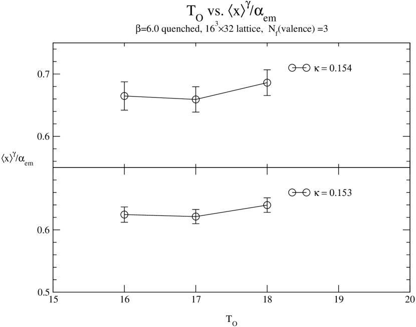
FIG. 1.: The first moment of $F_{2}^{\gamma}$ for $\beta$=6.0 quenched configurations for the different time position of the operator ($T_{\cal O}$).

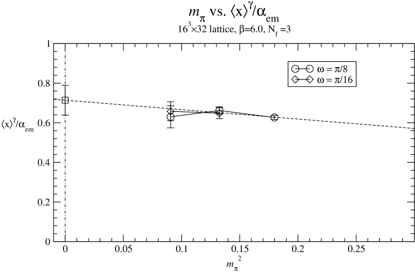
FIG. 2.: The first moment of $F_{2}^{\gamma}$ for $\beta$=6.0 quenched configurations $(a^{-1}\sim 2.4~{}$GeV). $\omega=\pi/8\ (\pi/16)$ correspond to the periodic (antiperiodic) boundary condition for the pseudofermion fields in the $z$ direction. $m_{\pi}$ is in lattice units ($a$ = 1).

REFERENCES

• [1] G. Martinelli and C. T. Sachrajda, Nucl. Phys. B306, 865 (1988);
G. Martinelli and C. T. Sachrajda, Nucl. Phys. B316,355 (1989).
• [2] M. Göckeler et al., Phys. Rev. D53,2317 (1996);
M. Göckeler et al., Phys. Rev. D56,2743 (1997).
• [3] D. Dolgov et al., Nucl. Phys. Proc. Suppl. 94, 303 (2001).
• [4] X. Ji and C. Jung, Phys. Rev. Lett. 86, 208 (2001).
• [5] S. J. Brodsky, T Kinoshita and H. Terazawa, Phys. Rev. D4 1532 (1971);
T. F. Walsh and P. M. Zerwas, Nucl. Phys. B41 551 (1972).
• [6] R. Nisius, Phys. Rept. 332,165 (2000);
M. Krawczyk, A. Zembrzuski and M. Staszel, hep-ph/0011083.
• [7] M. Stratmann, Nucl. Phys. Proc. Suppl. 82, 400 (2000);
M. Stratmann, hep-ph/9910318;
M. Stratmann and W. Vogelsang, Phys. Lett. B386, 370 (1996).
• [8] C. Peterson, T. F. Walsh and P. M. Zerwas, Nucl. Phys. B174, 424 (1980).
• [9] G. Kilcup, D. Pekurovsky and L. Venkataraman, Nucl. Phys. Proc. Suppl. 53, 345 (1997); L.Venkataraman and G. Kilcup, hep-lat/9711006.
• [10] M. Göckeler et al., Phys. Rev. D57, 5562 (1998) and the references therein.
• [11] S. Capitani and G. Rossi, Nucl. Phys. B433, 351 (1995);
G. Beccarini et al., Nucl. Phys. B445, 351 (1995);
M. Göckeler et al., Nucl. Phys. B472, 309 (1996).
• [12] T. F. Walsh and P. M. Zerwas, Phys. Lett. 44B 195 (1973);
R. L. Kingsley, Nucl. Phys. B60 45 (1973).
• [13] M. Glück, E. Reya and A. Vogt, Phys. Rev. D45, 3986 (1992); ibid. D46, 1973 (1992).
• [14] S. J. Dong, K. F. Liu and A. G. Williams, Phys. Rev. D58, 074504 (1998).