HOW TO CALCULATE THE BUBBLE NUCLEATION RATE IN FIRST ORDER TRANSITIONS NON-PERTURBATIVELY^∗

Abstract

We present a new method for calculating the bubble nucleation rate in first order phase transitions non-perturbatively on the lattice. The method takes into account all fluctuations and the full dynamical pre-factor. We also present results from applying it to the cubic anisotropy model, which has a radiatively induced, strongly first order phase transition.

Electroweak baryogenesis in the Standard Model (or extensions of it) happens on or near the surface of the bubbles which nucleate and subsequently grow during the first order Electroweak phase transition.[1] In this case, it is very difficult to compute the bubble nucleation rate analytically with sufficient accuracy: since the transition is radiatively generated, no classical bubble solution exists, and the whole idea of separating the classical bubble from the fluctuation determinant, needed for Langer’s nucleation theory,[2] becomes cumbersome. Furthermore, the long-distance physics of the Electroweak theory is inherently non-perturbative, making lattice simulations necessary.

How can one calculate the nucleation rate on the lattice? The most straightforward method is to take an ensemble of configurations in the metastable state, evolve each with Hamilton’s equations of motion, and wait for tunneling to happen. This has been done, for instance in the Ising model [3] and the $\phi^{4}$ model.[4] However, the cooling rate of the Universe during the Electroweak phase transition is many orders of magnitude smaller than the timescale of microscopic interactions. Thus, the system has plenty of time for probing its phase space, and the tunneling will happen through very strongly suppressed configurations ($p\sim e^{-100}$) after a small amount of supercooling. However, it is impossible to make Monte Carlo simulations with $e^{100}$ iterations!

Below, we shall describe a Monte Carlo method which fully overcomes this problem, and which can be used to calculate both the static and the dynamical parts of the nucleation rate. Instead of using the full $SU(2)\times U(1)+$Higgs, we chose as our toy model the cubic anisotropy model, which has the desired features:

$\bullet$ It has a radiatively induced, first order transition. As mentioned above, this makes analytical computations quite difficult, see ref.[5]

$\bullet$ It is simple to simulate on the lattice.

The continuum Hamiltonian of the cubic anisotropy model in three dimensions is ($\phi_{1}$ and $\phi_{2}$ are scalar fields, $\pi_{1}$ and $\pi_{2}$ the associated canonical momenta):

$${\mathcal{H}}=\sum_{a=1,2}\bigg{[}\frac{1}{2}\pi_{a}^{2}+\frac{1}{2}\partial_{i}\phi_{a}\partial_{i}\phi_{a}+\frac{1}{2}m^{2}\phi_{a}^{2}+\frac{\lambda_{1}}{24}\phi_{a}^{4}\bigg{]}+\frac{\lambda_{2}}{4}\phi_{1}^{2}\phi_{2}^{2}$$ (1)

The Hamiltonian is discretized on the lattice using an improved (next-to-nearest neighbour) Laplacian. Included also are loop corrections to second order, which enter in the lattice versions of $\lambda_{1}$, $\lambda_{2}$, $\phi_{1}$, $\phi_{2}$ and $m^{2}$. We fix $\lambda_{2}=8\lambda_{1}$, giving us a strongly first order phase transition between the symmetric and broken phases, as we vary $m^{2}$. In this case $m^{2}$ plays the role of the temperature. We find the critical $m^{2}$, $m^{2}_{c}$, the latent heat and the interface tension. The full results will be presented in a future paper.[6]

The calculation of the rate can be split up into two main parts, the static probability of the critical bubbles (part $I$), and the dynamical flux of the phase space through the bubble configurations (part $II$). As an order parameter, we choose the space average of $\Phi^{2}=\phi_{1}^{2}+\phi_{2}^{2}$.

• The non-dynamical part $I$ is the probability of having a critical bubble configuration. It is found by calculating the probability distribution $P(\Phi^{2})$ of the order parameter (see Fig. 1), and defining the critical bubble to be at the minimum, $Z$. We define a region $[Z-\frac{\epsilon}{2},Z+\frac{\epsilon}{2}]$ as the critical bubble region.

  At the critical temperature, because of the finiteness of the lattice, the most suppressed configurations are slabs (see Fig. 1), and the bubble configurations are found on the inner sides of the two peaks. Lowering the temperature ($m^{2}$), the critical bubble becomes smaller and eventually it will fit inside the lattice volume. Part I is then the probability density in the critical bubble region ($\frac{P_{z}}{\epsilon}$) divided by the probability of the metastable state ($P_{A}$).

  $$I = \frac{P_{z}}{P_{A}\epsilon}~{}~{},~{}~{}P_{Z}=\int_{Z-\frac{\epsilon}{2}}^{Z+\frac{\epsilon}{2}}P(\Phi^{2})d\Phi^{2}~{}~{},~{}~{}P_{A}=\int_{0}^{Z}P(\Phi^{2})d\Phi^{2}$$ (2)

  $P(\Phi^{2})$ is found by using multicanonical methods.[6] It can be reweighted to several different values of $m^{2}$, and part $I(m^{2})$ calculated.

  Figure 1: Sketch of the different geometries of the configurations in a finite box (left).The probability distribution is reweighted to several different values of $m^{2}$ where the critical bubble fits inside the lattice volume. For each $m^{2}$, $Z$ is determined and $\epsilon$ is chosen (right).

• Part $IIa$ is the flux of order parameter through the critical bubble value, $Z$. It can be calculated analytically[6]:

  $$IIa\equiv\frac{1}{2}\langle|\frac{d\Phi^{2}}{dt}|\rangle~{}=~{}\sqrt{\frac{2Z}{\pi V}}$$ (3)

• However, not all of the flux in $IIa$ leads to tunneling. The bubble wobbles back and forth for some time before falling into one of the minima. Since we are actually sampling the configurations  at $\Phi^{2}=Z$, we are over-counting the true phase space flux from the symmetric phase to the broken phase by the average number of crossings of $Z$ the trajectories make. Therefore, we use the Hamiltonian in Eq. (1) to calculate the real time trajectories forward and backwards in time from initial configurations in the critical bubble region $[Z-\frac{\epsilon}{2},Z+\frac{\epsilon}{2}]$. Gluing the two together into a full trajectory, we can then count the number of crossings, and determine whether the trajectory starts and ends in different minima. Finally, we can correct the part $IIa$ with part $IIb$:

  $$IIb \equiv \frac{1}{N}\sum_{i}\frac{\delta_{i}}{c_{i}}$$ (4)

  where $N$ is the number of trajectories, $c_{i}$ is the number of crossings of the i’th trajectory and $\delta_{i}$ is 1 if the trajectory tunneled, 0 if not.

  However, since the Hamiltonian evolution of the bubble conserves the total energy, the finite size of the system poses a problem: when the bubble grows (shrinks), it releases (absorbs) latent heat, and the temperature grows (decreases). This effect tends to unphysically “stabilize” the bubble around the critical radius, see Fig. 2. This can be solved by going to very large volumes, which is too expensive, or by adding a small amount of thermal noise in the system. The thermal noise consists of an update of the momenta:

  $$\pi^{\prime}=\sqrt{1-\epsilon^{2}}\pi+\epsilon\xi~{}~{},~{}~{}\epsilon=\sqrt{\frac{2\delta t}{L}}$$ (5)

  where $\xi$ is taken from a Gaussian of width 1. The amplitude of the noise is tuned so that the $\pi$’s are thermalized after evolution of length $t=\lambda_{2}aL$. The final rate is insensitive to the precise value of $\epsilon$.

  

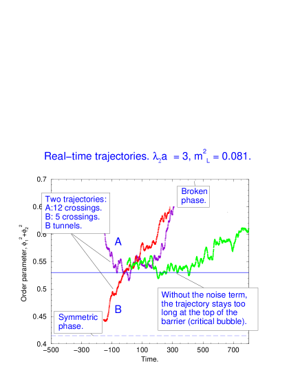
  Figure 2: From the trajectories we can count the crossings and see if it is a tunneling trajectory. Without the noise term, the bubble stays on the barrier too long and the number of crossings becomes too large.

The final rate is (see Figure 3):

$$\Gamma=\frac{I\times IIa\times IIb}{V}$$ (6)

In Fig. 3 we compare our result with the thin-wall approximation. At smallest supercoolings we have studied, the thin-wall result gives a rate $\sim 25$ orders of magnitude too large. However, for a fixed rate, the thin-wall approximation gives “only” $\sim 30$% too small supercooling $\delta m^{2}$.

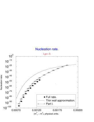
Figure 3: The full nucleation rate compared to the thin-wall approximation (line).

To conclude, we have described a lattice Monte Carlo method for calculating the full bubble nucleation rate in first order phase transitions. The method is especially well suited for transitions which happen through very strongly suppressed bubble configurations; indeed, most first order phase transitions in Nature fall into this class. We have applied this method to the cubic anisotropy model in 3D, for a full description we refer to the forthcoming paper.[6] This method has also been applied to $SU(2)$+Higgs theory, but with a heat bath evolution instead of the Hamiltonian real time evolution.[7]

References

References

- [1] A.E.Nelson, D.B.Kaplan, A.G.Cohen, Nucl.Phys, B373, p.453-478, (1992).
- [2] J.S.Langer, Ann. of Phys., 41, p108-167, (1967).
- [3] M.Acharyya, D.Stauffer, cond-mat/9801213
- [4] S.Borsanyi, A.Patkos, J.Polonyi, Z.Szep, hep-th/0004059.
- [5] A.Strumia, N.Tetradis, Nucl. Phys. B 554 (1999) 697.
- [6] G.D.Moore, K.Rummukainen, A.Tranberg, In preparation.
- [7] G.D.Moore, K.Rummukainen, hep-ph/0009132.