Abstract

The vacuum dynamics of SU(2) and SU(3) lattice gauge theories is studied by means of a gauge-invariant effective action defined using the lattice Schrödinger functional at finite temperature. In the case of the SU(3) gauge theory numerical simulations are performed at zero and finite temperature. The vacuum is probed using an external constant Abelian chromomagnetic field. At zero temperature, in agreement with our previous studies for the SU(2) theory, the external field is totally screened in the continuum limit. At finite temperature numerical data suggest that confinement is restored by increasing the strength of the applied field. We give also an estimate of the deconfinement temperature.

PACS number(s): 11.15.Ha

1. INTRODUCTION

The lattice approach to gauge theories allows the non-perturbative study of gauge systems without loosing the gauge invariance. Recently [1] it has been proposed a method to define on the lattice the gauge invariant effective action by using the Schrödinger functional [2, 3, 4, 5].
In the continuum the Euclidean Schrödinger functional in Yang-Mills theories without matter fields reads:

$${\mathcal{Z}}[A^{(f)},A^{(i)}]=\left\langle A^{(f)}\left|e^{-HT}{\mathcal{P}}\right|A^{(i)}\right\rangle\,.$$ (1.1)

In Eq. (1.1) $H$ is the pure gauge Yang-Mills Hamiltonian in the fixed-time temporal gauge, $T$ is the Euclidean time extension, while ${\mathcal{P}}$ projects onto the physical states. $A^{a(i)}_{k}(\vec{x})$ and $A^{a(f)}_{k}(\vec{x})$ are static classical gauge fields, and the state $|A\rangle$ is such that

$$\langle A|\Psi\rangle=\Psi[A]\,,$$ (1.2)

$\Psi[A]$ being a wavefunctional. Note that, by definition, ${\mathcal{Z}}[A^{(f)},A^{(i)}]$ is invariant under gauge transformations of the gauge fields $A^{(i)}$ and $A^{(f)}$.
Using standard formal manipulations and the gauge invariance of the Schrödinger functional it is easy to rewrite ${\mathcal{Z}}[A^{(f)},A^{(i)}]$ as a functional integral [2, 3, 4]

$${\mathcal{Z}}[A^{(f)},A^{(i)}]=\int{\mathcal{D}}A\;e^{-\int_{0}^{T}dx_{4}\,\int d^{3}x\,{\mathcal{L}}_{YM}(x)}$$ (1.3)

with the constraints:

$$A_{\mu}(x_{4}=0)= A^{(i)}_{\mu}$$

$$A_{\mu}(x_{4}=T)= A^{(f)}_{\mu}\;.$$

It is worthwhile to stress that in Eq. (1.3) we should sum over the topological inequivalent classes. However, it turns out [5] that on the lattice such an average is not needed because the functional integral in Eq. (1.3) is already invariant under arbitrary gauge transformation of $A^{(i)}$ and $A^{(f)}$. The lattice implementation of the Schrödinger functional Eq. (1.3) is given by [5]:

$${\mathcal{Z}}[U^{f},U^{i}]=\int{\mathcal{D}}U\;e^{-S}\,,$$ (1.5)

where the integrations over the links $U_{\mu}(x)$ are done with the fixed boundary conditions:

$$U(x)|_{x_{4}=0}=U^{(i)}\,,\quad U(x)|_{x_{4}=T}=U^{(f)}\,.$$ (1.6)

The links $U^{(i)}$ and $U^{(f)}$ are the lattice version of the continuum gauge fields $A^{(i)}$ and $A^{(f)}$.
In Ref. [1] we introduced the new functional:

$$\Gamma[\vec{A}^{\mathrm{ext}}]=-\frac{1}{T}\ln\left\{\frac{{\mathcal{Z}}[U^{\mathrm{ext}}]}{{\mathcal{Z}}(0)}\right\}\,,$$ (1.7)

where

$${\mathcal{Z}}[U^{\mathrm{ext}}]={\mathcal{Z}}[U^{\mathrm{ext}},U^{\mathrm{ext}}]\,,$$ (1.8)

and ${\mathcal{Z}}[0]$ means the Schrödinger functional Eq. (1.8) without external background field ($U^{\mathrm{ext}}_{\mu}=\mathbf{1}$).
From the previous discussion it is evident that ${\mathcal{Z}}[U^{\mathrm{ext}}]$ is invariant against lattice gauge transformations of the external link $U^{\mathrm{ext}}$. Moreover, it can be shown that [1]:

$$\lim_{T\to\infty}\Gamma[\vec{A}^{\mathrm{ext}}]=E_{0}[\vec{A}^{\mathrm{ext}}]-E_{0}[0]$$ (1.9)

where $E_{0}[\vec{A}^{\mathrm{ext}}]$ is the vacuum energy in presence of the external background field. Thus we see that $\Gamma[\vec{A}^{\mathrm{ext}}]$ is the lattice gauge-invariant effective action for the static background field $\vec{A}^{\mathrm{ext}}$. It is worthwhile to stress that our lattice effective action is defined by means of the lattice Schrödinger functional Eq. (1.5) with the same boundary fields at $x_{4}=0$ and $x_{4}=T$. As a consequence we have [1]:

$${\mathcal{Z}}[U^{\mathrm{ext}}]=\int{\mathcal{D}}U\;e^{-S_{W}}\;,$$ (1.10)

where $S_{W}$ is the familiar Wilson action and the functional integral is defined over a four-dimensional hypertorus with the “cold-wall” at $x_{4}=0$:

$$U_{\mu}(x)|_{x_{4}=0}=U^{\mathrm{ext}}_{\mu}\,.$$ (1.11)

In previous studies [6, 7, 8] we investigated the vacuum dynamics of the SU(2) lattice gauge theory by using an external constant Abelian chromagnetic field. In that case the relevant quantity is the density of effective action:

$$\varepsilon[\vec{A}^{\mathrm{ext}}]=-\frac{1}{\Omega}\ln\left[\frac{{\mathcal{Z}}[A^{\mathrm{ext}}]}{{\mathcal{Z}}[0]}\right]\,,$$ (1.12)

where $\Omega=V\cdot T$, $V$ being the spatial volume.
The aim of the present paper is twofold. First, we extend the study of the effective action with an external Abelian chromomagnetic field to the lattice SU(3) gauge theory at zero temperature. Second, we consider both SU(2) and SU(3) gauge systems at finite temperature.
At finite temperature the relevant quantity is the partition function :

$$\text{Tr}\left[e^{-\beta_{T}H}\right]=\int\mathcal{D}\vec{A}\,\langle\vec{A}\left|e^{-\beta_{T}H}\mathcal{P}\right|\vec{A}\rangle\,,$$ (1.13)

where $\beta_{T}$ is the inverse of the physical temperature. The thermal partition function Eq. (1.13) can be written as a functional integral [4]:

$$\text{Tr}\left[e^{-\beta_{T}H}\right]=\int_{A_{\mu}(\beta_{T},\vec{x})=A_{\mu}(0,\vec{x})}\mathcal{D}A_{\mu}(t,\vec{x})\,e^{-\int^{\beta_{T}}_{0}dx_{4}\,\int d^{3}\vec{x}\mathcal{L}_{Y-M}(\vec{x},x_{4})}\,.$$ (1.14)

The lattice implementation of Eq. (1.14) is straightforward. We have:

$$\text{Tr}\left[e^{-\beta_{T}H}\right]=\int_{U_{\mu}(\beta_{T},\vec{x})=U_{\mu}(0,\vec{x})=U_{\mu}(\vec{x})}\mathcal{D}U_{\mu}(x_{4},\vec{x})\,e^{-S_{W}}\,.$$ (1.15)

Note that, by comparing Eq. (1.15) with Eqs. (1.10), we have:

$$\text{Tr}\left[e^{-\beta_{T}H}\right]=\int\mathcal{D}U_{\mu}(\vec{x})\,\mathcal{Z}[U_{\mu}(\vec{x})]\,,$$ (1.16)

where $\mathcal{Z}[U_{\mu}(\vec{x})]$ is the Schrödinger functional Eq. (1.10) defined on a lattice with $L_{4}=\beta_{T}$, and “external” links $U_{\mu}(\vec{x})$ at $x_{4}=0$.
We are interested in the thermal partition function in presence of a given static background field $\vec{A}^{\mathrm{ext}}(\vec{x})$. In the continuum this can be obtained by splitting the gauge field into the background field $\vec{A}^{\mathrm{ext}}(\vec{x})$ and the fluctuating fields $\vec{\eta}(\vec{x})$. So that we could write formally:

$$\mathcal{Z}_{T}[\vec{A}^{\mathrm{ext}}]=\int\mathcal{D}\vec{\eta}\,\langle\vec{A}^{\mathrm{ext}},\vec{\eta}\left|e^{-\beta_{T}H}\mathcal{P}\right|\vec{A}^{\mathrm{ext}},\vec{\eta}\rangle\,.$$ (1.17)

The lattice implementation of Eq. (1.17) can be obtained from Eq. (1.15) if we write

$$U_{k}(\beta_{T},\vec{x})=U_{k}(0,\vec{x})=U^{\text{ext}}_{k}(\vec{x})\widetilde{U}_{k}(\vec{x})\,,$$ (1.18)

where $U^{\text{ext}}_{k}(\vec{x})$ is the lattice version of the external continuum field $\vec{A}^{\mathrm{ext}}$ and the $\widetilde{U}_{k}(\vec{x})$’s are the fluctuating links. Thus we get:

$$\mathcal{Z}_{T}[\vec{A}^{\mathrm{ext}}]=\int_{x_{4}=0}\mathcal{D}\widetilde{U}_{k}(\vec{x})\,\mathcal{D}{U}_{4}(\vec{x})\,\mathcal{Z}[U_{k}^{\text{ext}}(\vec{x}),\widetilde{U}_{k}(\vec{x})]\,.$$ (1.19)

Note that in Eq. (1.19) only the spatial links belonging to the hyperplane $x_{4}=0$ are written as the product of the external link $U^{\text{ext}}_{k}(\vec{x})$ and the fluctuating links $\widetilde{U}_{k}(\vec{x})$. The temporal links $U_{4}(x_{4}=0,\vec{x})$ are left freely fluctuating. It follows that the temporal links $U_{4}(x)$ satisfy the usual periodic boundary conditions. We stress that the periodic boundary conditions in the temporal direction are crucial to retain the physical interpretation that the functional $\mathcal{Z}_{T}[\vec{A}^{\text{ext}}]$ is a thermal partition function. In the following the spatial links belonging to the time-slice $x_{4}=0$ will be called “frozen links”, while the remainder will be the “dynamical links”. From the physical point of view we are considering the gauge system at finite temperature in interaction with a fixed external background field. As a consequence, in the Wilson action $S_{W}$ we keep only the plaquettes built up with the dynamical links or with dynamical and frozen links. With these limitations it is easy to see that in Eq. (1.19) we have:

$$\mathcal{Z}\left[U_{k}^{\text{ext}}(\vec{x}),\widetilde{U}_{k}(\vec{x})\right]=\mathcal{Z}\left[U_{k}^{\text{ext}}(\vec{x})\right]\,.$$ (1.20)

Indeed, let us consider an arbitrary frozen link $U^{\text{ext}}_{k}(\vec{x})\widetilde{U}_{k}^{\text{ext}}(\vec{x})$. This link enters in the modified Wilson action by means of the plaquette:

$$P_{k4}(x_{4}=0,\vec{x})=\text{Tr}\left\{U^{\text{ext}}_{k}(\vec{x})\widetilde{U}_{k}^{\text{ext}}(\vec{x})U_{4}(0,\vec{x}+\hat{k})U^{\dagger}_{k}(1,\vec{x}+\hat{k})U^{\dagger}_{4}(0,\vec{x})\right\}\,.$$ (1.21)

Now we observe that the link $U_{4}(0,\vec{x}+\hat{k})$ in Eq. (1.21) is dynamical, i.e. we are integrating over it. So that, by using the invariance of the Haar measure we obtain:

$$P_{k4}(x_{4}=0,\vec{x})=\text{Tr}\left\{U^{\text{ext}}_{k}(\vec{x})U_{4}(0,\vec{x}+\hat{k})U^{\dagger}_{k}(1,\vec{x}+\hat{k})U^{\dagger}_{4}(0,\vec{x})\right\}\,.$$ (1.22)

It is evident that Eq. (1.22) in turns implies Eq. (1.20). Then, we see that in Eq. (1.19) the integration over the fluctuating links $\widetilde{U}_{k}(\vec{x})$ gives an irrelevant multiplicative constant. So that we obtain:

$$\mathcal{Z}_{T}\left[\vec{A}^{\text{ext}}\right]=\int_{U_{k}(\beta_{T},\vec{x})=U_{k}(0,\vec{x})=U^{\text{ext}}_{k}(\vec{x})}\mathcal{D}U\,e^{-S_{W}}\,,$$ (1.23)

where the integrations are over the dynamical links with periodic boundary conditions in the time direction. As concern the boundary conditions at the spatial boundaries, we keep the fixed boundary conditions $U_{k}(\vec{x},x_{4})=U_{k}^{\text{ext}}(\vec{x})$ used in the Schrödinger functional Eq. (1.10). We stress that, if we send the physical temperature to zero, then the thermal functional Eq. (1.23) reduces to the zero-temperature Schrödinger functional Eq. (1.5) with the constraints $U_{k}(x)|_{x_{4}=0}=U^{\mathrm{ext}}_{k}(\vec{x})$ instead of Eq. (1.11). In our previous studies [1, 6, 7, 8] we checked that in the thermodynamic limit both conditions agree as concern the zero-temperature effective action Eq. (1.7).
The plan of the paper is as follows. In Section 2 we consider the Abelian constant chromomagnetic background field for the pure gauge SU(3) lattice theory at zero temperature. Section 3 is devoted to the study of both SU(2) and SU(3) lattice theories at finite temperature in presence of the external background field. Finally our conclusions are drawn in Section 4.

2. SU(3) IN A CONSTANT CHROMOMAGNETIC FIELD

We are interested in the case of a constant Abelian chromomagnetic field which in the continuum reads:

$$\vec{A}^{\mathrm{ext}}_{a}(\vec{x})=\vec{A}^{\mathrm{ext}}(\vec{x})\delta_{a,3}\,,\quad\vec{A}^{\mathrm{ext}}_{k}(\vec{x})=\delta_{k,2}x_{1}H\,.$$ (2.1)

The lattice links corresponding to $\vec{A}^{\mathrm{ext}}(\vec{x})$ can be evaluated from:

$$U_{\mu}={\mathrm{P}}\exp\left\{ig\int_{0}^{1}dt\,A_{\mu}(x+t\hat{\mu})\right\}$$ (2.2)

where ${\mathrm{P}}$ is the path-ordering operator, and $A_{\mu}=A_{\mu}^{a}\frac{\lambda^{a}}{2}$, the $\lambda^{a}$’s being the Gell-Mann matrices. From Eqs. (2.1) and (2.2) we get:

$$U^{\mathrm{ext}}_{1}(\vec{x})= U^{\mathrm{ext}}_{3}(\vec{x})=U^{\mathrm{ext}}_{4}(\vec{x})={\mathbf{1}}$$

$$U^{\mathrm{ext}}_{2}(\vec{x})= \begin{bmatrix}e^{i\frac{gHx_{1}}{2}}&0&0\\ 0&e^{-i\frac{gHx_{1}}{2}}&0\\ 0&0&1\end{bmatrix}\;\,.$$ (2.3)

Our Schrödinger functional Eq. (1.10) is defined on a lattice with the hypertorus geometry, for it is natural to impose that:

$$U_{2}(x_{1},x_{2},x_{3},x_{4})=U_{2}(x_{1}+L_{1},x_{2},x_{3},x_{4})\,,$$ (2.4)

where $L_{1}$ is the lattice extension in the $x_{1}$ direction (in lattice units). As a consequence the magnetic field $H$ turns out to be quantized:

$$\frac{gH}{2}=\frac{2\pi}{L_{1}}n_{\mathrm{ext}}\,,$$ (2.5)

with $n_{\mathrm{ext}}$ integer.
According to the discussion of the previous Section, in evaluating the lattice functional integral Eq. (1.10) we impose that links belonging to the time slice $x_{4}=0$ are frozen to the configuration Eq. (2.). Moreover we impose also that the links at the spatial boundaries are fixed according to Eq. (2.). In the continuum this last condition amounts to the usual requirement that the fluctuations over the background fields vanish at infinity.
An alternative possibility is given by constraining the links belonging to the the time slice $x_{4}=0$ and those at the spatial boundaries to the condition

$$U_{k}(x)=U_{k}^{\mathrm{ext}}(\vec{x})\,,\qquad k\,=\,1,2,3$$ (2.6)

while the links $U_{4}(x)$ are unconstrained. Note that with the condition Eq. (2.6) the time-like plaquettes nearest the frozen hypersurface $x_{4}=0$ behave symmetrically in the update procedure. Moreover, in this way the Schrödinger functional Eq. (1.10) is the zero-temperature limit of the thermal partition functional Eq. (1.23). In our previous studies [6, 7, 8] we checked that in the thermodynamic limit both conditions agree as the effective action is concerned.
Our numerical simulations at zero temperature have been done on a lattice of size $L_{1}L_{2}L_{3}L_{4}$ with $L_{1}=L_{4}=32$, while the transverse size $L_{1}=L_{2}=L_{\perp}$ has been varied from $L_{\perp}=8$ up to $L_{\perp}=32$. To avoid the problem of computing a partition function which is the exponential of an extensive quantity we consider the derivative of the density of effective action $\varepsilon[\vec{A}^{\mathrm{ext}}]$ Eq. (1.12) with respect to $\beta$ by taking $n_{\mathrm{ext}}$ (i.e. $gH$) fixed. Indeed, we have

$$\varepsilon^{\prime}[\vec{A}^{\mathrm{ext}}]=\frac{\partial\varepsilon[\vec{A}^{\mathrm{ext}}]}{\partial\beta}=-\frac{1}{\Omega}\left[\frac{1}{{\mathcal{Z}}[U^{\mathrm{ext}}]}\frac{\partial{\mathcal{Z}}[U^{\mathrm{ext}}]}{\partial\beta}\right.$$ (2.7)

$$\left.-\frac{1}{{\mathcal{Z}}[0]}\frac{\partial{\mathcal{Z}}[0]}{\partial\beta}\right]=\left\langle\frac{1}{\Omega}\sum_{x,\mu>\nu}\frac{1}{3}\,{\mathrm{Re}\,\mathrm{Tr}}U_{\mu\nu}(x)\right\rangle_{0}$$

$$-\left\langle\frac{1}{\Omega}\sum_{x,\mu>\nu}\frac{1}{3}\,{\mathrm{Re}\,\mathrm{Tr}}U_{\mu\nu}(x)\right\rangle_{\vec{A}^{\mathrm{ext}}}\,,$$

where the subscripts on the average indicate the value of the external links at the boundaries, and the $U_{\mu\nu}(x)$’s are the plaquettes in the $(\mu,\nu)$ plane. Actually, the contributions to $\varepsilon^{\prime}[\vec{A}^{\mathrm{ext}}]$ due to the frozen time-slice at $x_{4}=0$ and the fixed links at the spatial boundaries must be subtracted. Accordingly, we define the derivative of the internal energy density:

$$\varepsilon^{\prime}_{\mathrm{int}}[\vec{A}^{\mathrm{ext}}]=\left\langle\frac{1}{\Omega_{\mathrm{int}}}\sum_{x\in\tilde{\Lambda},\mu>\lambda}\frac{1}{3}\,{\mathrm{Re}\,\mathrm{Tr}}U_{\mu\nu}(x)\right\rangle_{0}$$ (2.8)

$$-\left\langle\frac{1}{\Omega_{\mathrm{int}}}\sum_{x\in\tilde{\Lambda},\mu>\lambda}\frac{1}{3}\,{\mathrm{Re}\,\mathrm{Tr}}U_{\mu\nu}(x)\right\rangle_{\vec{A}^{\mathrm{ext}}}\,,$$

where $\tilde{\Lambda}$ is the ensemble of the internal lattice sites which occupy the volume $\Omega_{\mathrm{int}}$.
To implement the constraint at the boundaries in the numerical simulations we update only the internal links, i.e. the links $U_{\mu}(x)$ with $x\in\tilde{\Lambda}$. We use the over-relaxed heat-bath algorithm to update the gauge configurations. Simulations have been performed by means of the APE100 computer. Since we are measuring a local quantity such as the plaquette, a low statistics (from 1000 up to 5000 configurations) is required in order to get a good estimate of $\varepsilon^{\prime}_{\mathrm{int}}$.

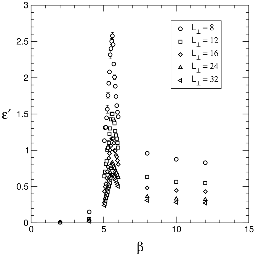
Figure 1: The $\beta$-derivative of the internal energy density Eq. (2.8) versus $\beta$ for SU(3) on a $L\times L_{\perp}^{2}\times L$ lattice. Plotted data refer to $L=32$ and different values of the transverse lattice size $L_{\perp}$.

In Figure 1 we display the derivative of the energy density normalized to the derivative of the external energy density:

$$\varepsilon^{\prime}_{\mathrm{ext}}=\frac{2}{3}\,[1-\cos(\frac{gH}{2})]=\frac{2}{3}\,[1-\cos(\frac{2\pi}{L_{1}}n_{\mathrm{ext}})]$$ (2.9)

versus $\beta$ for $L_{1}=L_{4}=32$ and $8\leq L_{\perp}\leq 32$. From Figure 1 we see that, as in the SU(2) gauge theory [6, 7, 8], both the peak and the perturbative plateau of $\varepsilon^{\prime}_{\mathrm{int}}$ decrease by increasing $L_{\perp}$. In order to perform the thermodynamic limit we introduce the scaling variable:

$$x=\frac{a_{H}}{L_{\mathrm{eff}}}\,,$$ (2.10)

where

$$a_{H}=\sqrt{\frac{2\pi}{gH}}$$ (2.11)

is the magnetic length, and

$$L_{\mathrm{eff}}=\Omega_{\mathrm{int}}^{1/4}$$ (2.12)

is the lattice effective linear size. As in the SU(2) case [8] we try the scaling law:

$$x^{-\alpha}\frac{\varepsilon^{\prime}_{\mathrm{int}}(\beta,n_{\mathrm{ext}},L_{\mathrm{eff}})}{\varepsilon^{\prime}_{\mathrm{ext}}}=\kappa(\beta)\,.$$ (2.13)

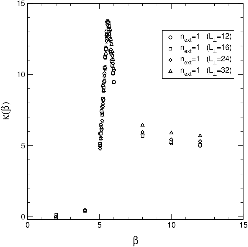
Figure 2: The scaling curve for SU(3) obtained by re-scaling all lattice data for $\varepsilon^{\prime}_{\mathrm{int}}(\beta,n_{\mathrm{ext}},L_{\mathrm{eff}})$ according to Eq. (2.13).

Indeed, from Figure 2 we see that our numerical data can be arranged on the scaling curve $\kappa(\beta)$. It is remarkable that the value of the exponent $\alpha=1.5$ in Eq. (2.13) agrees with the one we found for the SU(2) gauge theory [6, 7, 8]. From Eq. (2.13) we can determine the infinite volume limit of the vacuum energy density $\varepsilon_{\mathrm{int}}$. We have:

$$\lim_{L_{\mathrm{eff}}\to\infty}\varepsilon_{\mathrm{int}}(\beta,n_{\mathrm{ext}},L_{\mathrm{eff}})=\varepsilon^{\prime}_{\mathrm{ext}}\,\int_{0}^{\beta}d{\beta^{\prime}}\,\kappa(\beta^{\prime})\lim_{L_{\mathrm{eff}}\to\infty}\left(\frac{a_{H}}{L_{\mathrm{eff}}}\right)^{\alpha}=0$$ (2.14)

in the whole range of $\beta$. As a consequence, in the continuum limit $(L_{\mathrm{eff}}\to\infty,\beta\to\infty)$ the SU(3) vacuum screens the external chromomagnetic Abelian field in accordance with the dual superconductivity scenario [9, 10].

3. FINITE TEMPERATURE BACKGROUND FIELD EFFECTIVE ACTION

Let us consider the gauge systems in an external chromomagnetic Abelian field at finite temperature. According to the discussion in Section 1, we are interested in the thermal partition function $\mathcal{Z}_{T}\left[\vec{A}^{\text{ext}}\right]$, Eq. (1.23). On the lattice the physical temperature $T_{physical}$ is given by:

$$\frac{1}{T_{physical}}\,=\,L_{t}$$ (3.1)

where $L_{t}=L_{4}$ is the linear extension in the time direction. In order to approximate the thermodynamic limit, the spatial extension $L_{s}$ should respect the relation:

$$L_{s}\,\gg\,L_{t}\,.$$ (3.2)

To this end we perform our numerical simulation on $32^{3}\times L_{t}$ and $64^{3}\times L_{t}$ lattices by imposing:

$$\frac{L_{t}}{L_{s}}\,\leq\,4\,.$$ (3.3)

At finite temperature the effective action is defined through the free energy:

$$F[\vec{A}^{\mathrm{ext}}]=-\frac{1}{L_{t}}\ln\left\{\frac{\mathcal{Z}_{T}\left[\vec{A}^{\text{ext}}\right]}{{\mathcal{Z}_{T}}(0)}\right\}\,.$$ (3.4)

Obviously, in the case of constant external chromagnetic field the relevant quantity is the density of effective action:

$$f[\vec{A}^{\mathrm{ext}}]\,=\,\frac{1}{V}\,F[\vec{A}^{\mathrm{ext}}]\,.$$ (3.5)

As is well known, by increasing the temperature the pure gauge system undergoes the deconfinement phase transition. In the case of pure SU(N) gauge theories it is known that the expectation value of the Polyakov loop in the time direction

$$P=\frac{1}{V_{s}}\sum_{\vec{x}}\frac{1}{N}{\text{Tr}}\prod_{x_{4}=1}^{L_{t}}U_{4}(\vec{x},x_{4})$$ (3.6)

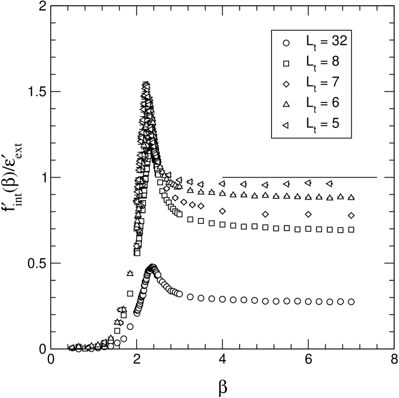
Figure 4: The $\beta$-derivative of the free energy density Eq. (3.5) for SU(2) on $L_{s}^{3}\times L_{t}$ lattices, with $L_{s}=32$.

is the order parameter for the deconfinement phase transition. As a preliminary step we look at the behavior of the temporal Polyakov loop versus the external applied field. We start with the SU(2) gauge system at $\beta=2.5$ on $32^{3}\times 5$ lattice at zero applied external field (i.e. $n_{\mathrm{ext}}=0$) that is known to be in the deconfined phase of finite temperature SU(2). If the external field strength is increased the expectation value of the Polyakov loop is driven towards the value at zero temperature (see Fig. 3). It is worthwhile to stress that this last result is consistent with the dual superconductor mechanism of confinement. Similar behavior has been reported by Authors of Refs. [11, 12] within a different approach. If we now consider the SU(2) gauge system at zero temperature in a constant Abelian chromomagnetic background field of fixed strength ($n_{\mathrm{ext}}=1$) and increase the temperature, we find that the perturbative tail of the $\beta$-derivative of the free energy density $f^{\prime}_{\mathrm{int}}(\beta,n_{\mathrm{ext}})/\varepsilon^{\prime}_{\mathrm{ext}}$ increases with $1/L_{t}$ and tends towards the “classical” value $f^{\prime}_{\mathrm{int}}(\beta,n_{\mathrm{ext}})/\varepsilon^{\prime}_{\mathrm{ext}}\simeq 1$ (see Fig. 4). Therefore we may conclude that, as the temperature increases, there is no screening effect in the free energy density, confirming that the zero-temperature screening of the external field is related to the confinement.

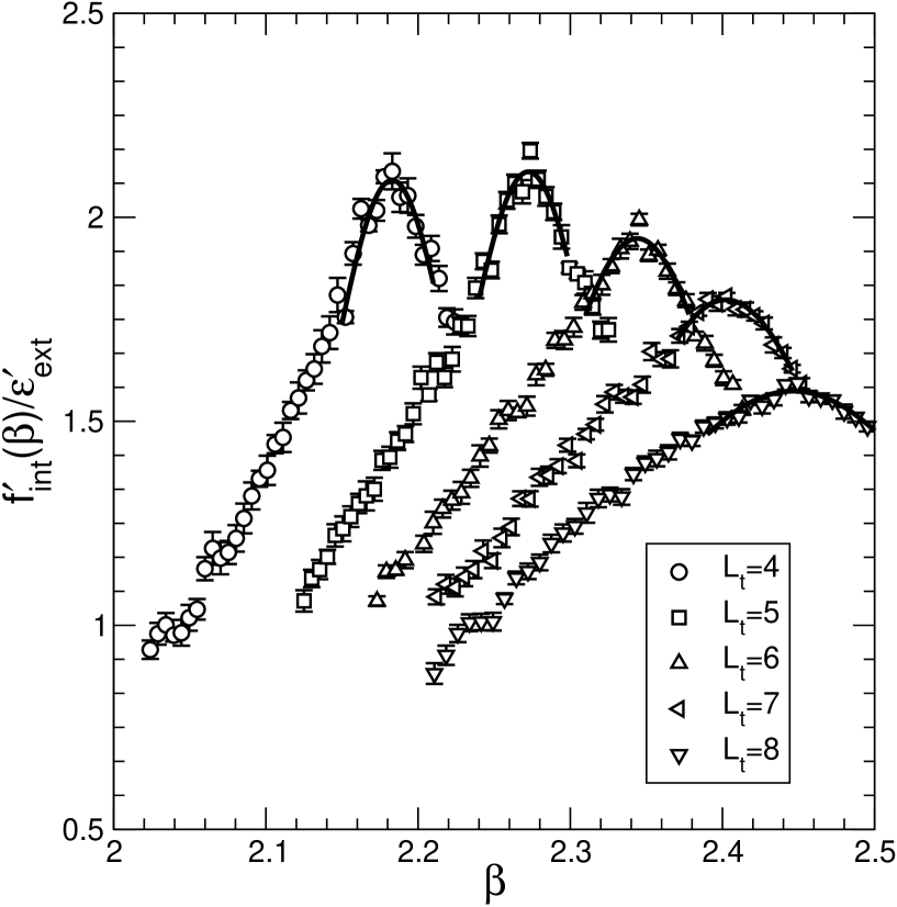
Figure 5: The peak region for the $\beta$-derivative of the free energy density Eq. (3.5) for SU(2). The data are taken on $L_{s}^{3}\times L_{t}$ lattices, with $L_{s}=64$. Solid lines are the best fits to the data using Eq. (3.7).

The knowledge of $f^{\prime}_{\mathrm{int}}(\beta,n_{\mathrm{ext}})/\varepsilon^{\prime}_{\mathrm{ext}}$ at finite temperature can be used to estimate the deconfinement temperature $T_{c}$. In Figure 5 we magnify the peak region for different values of $L_{t}$. We see clearly that the pseudocritical coupling $\beta^{*}(L_{t})$ depends on $L_{t}$. To determine the pseudocritical couplings we parametrize $f^{\prime}_{\mathrm{int}}(\beta,L_{t})$ near the peak as:

$$\frac{f^{\prime}_{\mathrm{int}}(\beta,L_{t})}{\varepsilon^{\prime}_{\mathrm{ext}}}=\frac{a_{1}(L_{t})}{a_{2}(L_{t})[\beta-\beta^{*}(L_{t})]^{2}+1}\,.$$ (3.7)

We restrict the region near $\beta^{*}(L_{t})$ until the fits Eq. (3.7) give a reduced $\chi^{2}/{\text{d}.o.f.}\sim 1$.
Having determined $\beta^{*}(L_{t})$ we estimate the deconfinement temperature as:

$$\frac{T_{c}}{\Lambda_{\mathrm{latt}}}=\frac{1}{L_{t}}\frac{1}{f(\beta^{*}(L_{t}))}\,,$$ (3.8)

where

$$f(\beta)=\left(\frac{\beta}{2Nb_{0}}\right)^{51/121}\,\exp\left(-\beta\frac{1}{4Nb_{0}}\right)\,,$$ (3.9)

where $b_{0}=(11N)/(48\pi^{2})$ and $N$ is the color number. In Figure 6 we display $T_{c}/\Lambda_{\mathrm{latt}}$ for different temperatures. Following Ref. [13] we linearly extrapolate to the continuum our data for $T_{c}/\Lambda_{\mathrm{latt}}$. In this way we obtain the following estimate of the critical temperature in the continuum limit

$$\frac{T_{c}}{\Lambda_{\mathrm{latt}}}\,=\,28.36\,\pm\,1.38\,.$$ (3.10)

Equation (3.10) is to be compared with the continuum limit of the critical temperature available in the literature [13]

$$\frac{T_{c}}{\Lambda_{\mathrm{latt}}}\,=\,24.38\,\pm\,2.18\,.$$ (3.11)

Our result Eq. (3.10) agrees, within two standard deviations, with the result given in Eq. (3.11). Note, however, that the small discrepancy could be a true dynamical effect due to the external chromomagnetic field. Indeed, the behaviour of the Polyakov loop versus the external background field displayed in Fig. 3 seems to suggest that the critical temperature does depend on the applied background field. For dimensional reasons one expects that:

$$T_{c}^{2}\,\,\sim\,\,H\,.$$ (3.12)

To check the expected behaviour Eq. (3.12) we need to vary the external chromomagnetic field. We plan to do this study in a future work.
For the time being, let us turn to the SU(3) pure gauge lattice theory at finite temperature. In this paper we limit ourselves to present our determination of the critical deconfinement temperature. In Figure 7 we display the peak region of the internal free energy density for different values of $L_{t}$, together with the fits Eq. (3.7). Having determined the pseudocritical couplings, the deconfinement temperature can be obtained from Eq.(3.8). Performing the linear extrapolation to the continuum limit we get:

$$\frac{T_{c}}{\Lambda_{\mathrm{latt}}}\,=\,20.86\,\pm\,3.02\,.$$ (3.13)

Our estimate Eq. (3.13) is in fair agreement with the continuum limit of the SU(3) critical temperature available in the literature [13]

$$\frac{T_{c}}{\Lambda_{\mathrm{latt}}}\,=\,29.67\,\pm\,5.47\,.$$ (3.14)

However, we note once more that our data do not exclude a dependence of the critical temperature on the external chromomagnetic field.

4. CONCLUSIONS

We have studied the non-perturbative dynamics of the vacuum of SU(2) and SU(3) lattice gauge theories by means of a gauge-invariant effective action defined using the lattice Schrödinger functional.

At zero temperature our numerical results indicate that even for the more interesting case of the SU(3) theory, in the continuum limit $L_{\mathrm{eff}}\to\infty$, $\beta\to\infty$ we have:

$$\varepsilon[\vec{A}^{\mathrm{ext}}]=0\,,$$ (4.1)

so that the SU(3) vacuum screens completely the external chromomagnetic Abelian field. In other words, the continuum vacuum behaves as an Abelian magnetic condensate medium in accordance with the dual superconductivity scenario.

The intimate connection between the screening of the external background field and the confinement is corroborated by the finite temperature results. Indeed our numerical data show that the zero-temperature screening of the external field is removed by increasing the temperature. Moreover, at finite temperature it seems that confinement is restored by increasing the strength of the external applied field.

At finite temperature we find that the $\beta$-derivative of the free energy density behaves like a specific heat. From the peak position of the $\beta$-derivative of the free energy density we obtained an estimate of the critical temperature $T_{c}/\Lambda_{\mathrm{latt}}$ that extrapolates in the continuum limit to values in fair agreement with previous determinations in the literature. Moreover, our data are suggestive of a non-trivial dependence of the deconfinement critical temperature on the applied external chromagnetic field. We deserve to a future work the investigation of this interesting possibility.

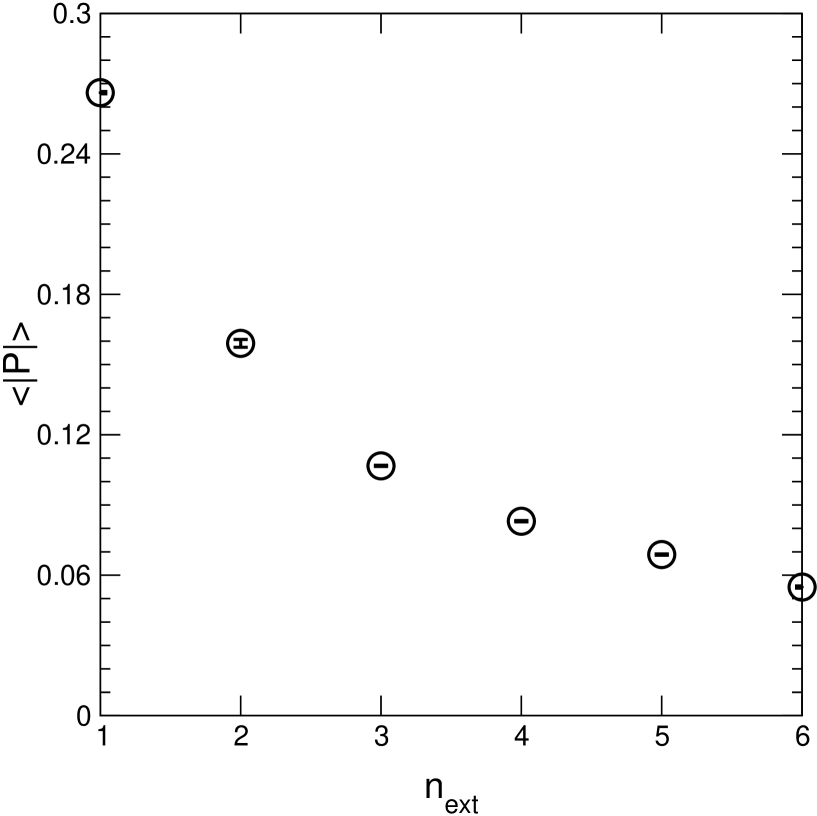
Figure 3: The absolute value of the Polyakov loop versus $n_{\mathrm{ext}}$, for SU(2), on a $32^{3}\times 5$ lattice at $\beta=2.5$.

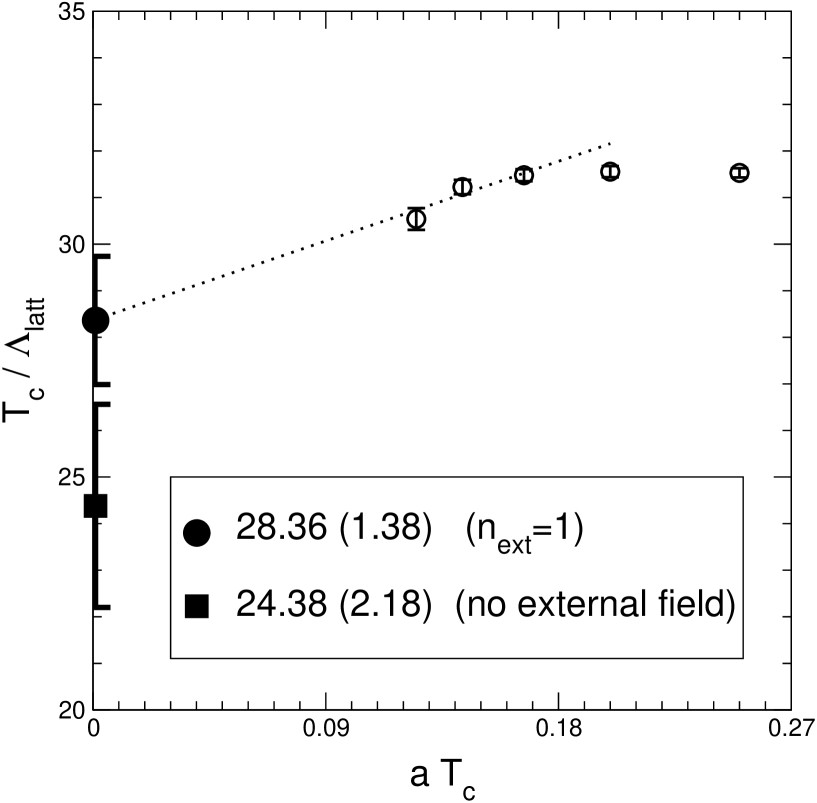
Figure 6: Our SU(2) lattice data for $T_{c}/\Lambda_{\mathrm{latt}}$ versus the temperature (circles). The full square is the continuum extrapolation of Ref. [13] (see Eq. (3.11)). The dotted line is a linear fit to our data.

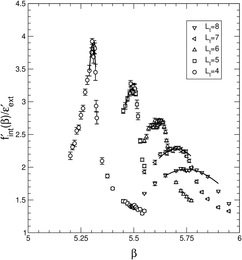
Figure 7: The peak region for the $\beta$-derivative of the free energy density Eq. (3.5) for SU(3). The data are taken on $L_{s}^{3}\times L_{t}$ lattices, with $L_{s}=64$. Solid lines are the best fits to the data using Eq. (3.7).

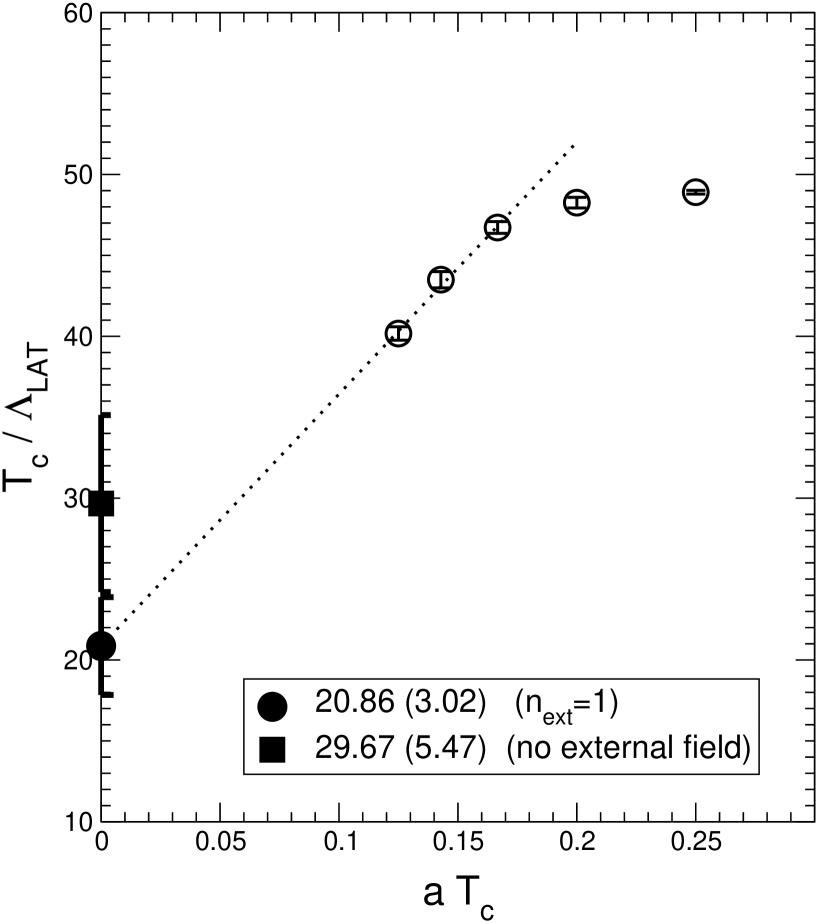
Figure 8: Our SU(3) lattice data for $T_{c}/\Lambda_{\mathrm{latt}}$ versus the temperature (circles). The full square is the continuum extrapolation of Ref. [13] (see Eq. (3.14)). The dotted line is a linear fit to our data.

References

- [1] P. Cea, L. Cosmai, and A. D. Polosa, Phys. Lett. B392, 177 (1997), hep-lat/9601010.
- [2] G. C. Rossi and M. Testa, Nucl. Phys. B176, 477 (1980).
- [3] G. C. Rossi and M. Testa, Nucl. Phys. B163, 109 (1980).
- [4] D. J. Gross, R. D. Pisarski, and L. G. Yaffe, Rev. Mod. Phys. 53, 43 (1981).
- [5] M. Lüscher, R. Narayanan, P. Weisz, and U. Wolff, Nucl. Phys. B384, 168 (1992), hep-lat/9207009.
- [6] P. Cea and L. Cosmai, Mod. Phys. Lett. A13, 861 (1998), hep-lat/9610028.
- [7] P. Cea and L. Cosmai, Nucl. Phys. Proc. Suppl. 73, 641 (1999), hep-lat/9809042.
- [8] P. Cea and L. Cosmai, Phys. Rev. D60, 094506 (1999), hep-lat/9903005.
- [9] G. ’t Hooft, in High Energy Physics, EPS International Conference, Palermo, 1975.
- [10] S. Mandelstam, Phys. Rept. 23, 245 (1976).
- [11] P. N. Meisinger and M. C. Ogilvie, Phys. Lett. B407, 297 (1997), hep-lat/9703009.
- [12] M. Ogilvie, Nucl. Phys. Proc. Suppl. 63, 430 (1998), hep-lat/9709127.
- [13] J. Fingberg, U. Heller, and F. Karsch, Nucl. Phys. B392, 493 (1993), hep-lat/9208012.