Algebraic Multigrid for Disordered Systems
and Lattice Gauge Theories

Abstract

The construction of multigrid operators for disordered linear lattice operators, in particular the fermion matrix in lattice gauge theories, by means of algebraic multigrid and block LU decomposition is discussed. In this formalism, the effective coarse-grid operator is obtained as the Schur complement of the original matrix. An optimal approximation to it is found by a numerical optimization procedure akin to Monte Carlo renormalization, resulting in a generalized (gauge-path dependent) stencil that is easily evaluated for a given disorder field. Applications to preconditioning and relaxation methods are investigated.

I Introduction

Most of the computer time in lattice gauge theory simulations is spent today on inverting the Dirac matrix, which describes the dynamics of quarks. While this problem can be tackled efficiently by iterative solvers such as Krylov subspace methods heplat-9404013 ; heplat-9608074 ; gutknecht-wup-1999 , these solvers suffer from critical slowing down in the physically interesting regions of small quark masses. One of the limiting factors here is that the elementary operation in iterative solvers, the matrix-vector multiplication, affects only next neighbors and thus limits the speed of information propagation over the lattice (though it can be improved by ILU preconditioning heplat-9602019 ; heplat-0011080 ). Using multigrid methods, one attempts to overcome this limitation by propagating information on a hierarchy of coarser and coarser grids.

Multigrid methods hackbusch-springer ; mccormick-siam for the Dirac matrix inversion were inspired by Mack’s multigrid approach to quantum field theory mack-1988 and have been proposed and investigated around 1990 by groups in Boston prd-43-1965 ; brower-moriarty-rebbi-vicari ; brower-edwards-rebbi-1991 ; vyas-jue-1991 ; prd-vyas , Israel plb-253-185 ; solomon-jue-1991 ; heplat-9204014 ; lauwers-benav-solomon-1992 , Amsterdam hulsebos-jue-1991 ; npb-331-531 ; plb-272-81 ; amsterdam-1991 , and Hamburg kalkreuter-jue-1991 ; heplat-9304004 ; heplat-9310029 ; heplat-9409008 ; heplat-9408013 ; thesis-baeker . Though it was shown that multigrid methods would, in principle, greatly reduce or eliminate critical slowing down, they have not been able to improve the performance of the Dirac matrix inversion in actual applications. These classical multigrid methods are based on a geometrical blocking of the lattice that leads to an effective coarse-grid formulation of the original matrix by a Galerkin approach. The choice of the blocking and interpolation kernels is crucial for the performance of the multigrid algorithm; they must be chosen such that the long-range and short-range dynamics decouple as much as possible. An optimal choice of the blocking kernels thus depends on the gauge field and must in principle be recalculated for each gauge configuration as the solution of a minimization problem. As this is not feasible, various approximations have been introduced in the literature.

Since then, the algebraic multigrid method siam-ruge-stueben ; reusken-wup-1999 ; notay-wup-1999 ; brandt-2000 ; zhang-2000 has emerged as a proven new method in numerical mathematics which does not rely on a geometrical decomposition of the lattice, but solely on the matrix itself. It starts out from a thinned lattice that contains a certain subset of the original lattice sites retaining their original values and constructs an effective operator on this lattice by means of an block $LU$ decomposition. Thus, instead of geometric proximity, the actual matrix elements determine in the coarsening procedure. For lattice gauge theory, this would automatically take the dynamics of the gauge field, which appears as a phase factor in the matrix elements, into account. (A similar reasoning was already cited by Edwards, Goodman, and Sokal prl-61-1333 in one of the first papers on multigrid methods for disordered systems, namely on random resistor networks, though it was later assumed that algebraic multigrid would be much more costly than the geometric variant heplat-9204014 .) Recently, algebraic multigrid was applied to lattice gauge theory by Medeke medeke-wup-1999 , and conversely research about renormalization-group improved and perfect operators in lattice gauge theory has been used to obtain efficient coarse-graining schemes for partial and stochastic differential equations condmat-0009449 .

One advantage of algebraic multigrid over geometric methods is that it directly gives a prescription for calculating the coarse-lattice operator and the interpolation kernel by a submatrix inversion problem. For this purpose, it is instructive to consider the problem of matrix inversion not in terms of the spectral decomposition, but in terms of the von Neumann series kuti-neumann-series ; vyas-random-walk . Combined with the block $LU$ decomposition, this results in a simple computational picture of the method as a noninteracting random walk on a hierarchically decomposed lattice in a disordered background. The resulting algebra of paths on this lattice is the basis for the computational construction of multigrid operators below, where the expansion coefficients are calculated numerically in a process similar to Monte Carlo renormalization. In that way, physical (or rather, computational) information about the fine-lattice operator is harvested to approximate the coarse-lattice operator as closely as desired.

The lattice fermion matrix is an example of the more general problem of disordered matrices operators which has many applications in different fields of computational physics. Some recent instances in the literature are e.g. the transport properties of light particles in solid-state physics kehr-1996 ; guo-miller-2000 , or transport in porous media, where multigrid methods have already been employed moulton-knapek-dendy-1998 ; SKnapek:99b . The numerical method investigated here is sufficiently general to be applicable to such problems.

Another factor that might turn out in favor of multigrid algorithms comes from recent advances in computer technology. Supercomputer architecture has long been dominated by vector-oriented machines that can quickly execute relatively simple and uniform elementary operations on large vectors. But because processor speed advances much faster than memory access speed, the performance of such operations is now severely limited by memory bandwidth. In computer architecture, this is overcome by using cache-oriented architectures such as in modern microprocessors, from which e.g. cluster computers iwcc-melbourne are built. These architectures are efficient for algorithms that have a high balance, i.e. number of operations per memory access, and make a frequent reuse of memory locations iwcc-melbourne-cbest ; cs-0007027 , but can tolerate much more complexity and irregularity. Multigrid algorithms usually result in denser, but smaller matrices and might thus be favored by these architectures.

Finally, problems other than matrix inversion have recently come into focus for the Dirac operator. One is the calculation of its low-lying eigenvalues, which was one of the first applications of multigrid heplat-9408013 and is today used for investigating hadron structure heplat-9709130 and chiral properties heplat-0010049 ; heplat-0003021 . Another one is the development of chirally-improved Dirac operators such as the Neuberger operator heplat-9806025 ; jansen-wup-1999 which requires the calculation of the inverse square root of a matrix. Algorithms for this problem are still under development, but as they also employ iterative solvers, it can be hoped that multigrid operators can aid in improving performance there. Multigrid methods have also been cited as a possible improvement to the domain-wall formulation of lattice gauge theory on a five-dimensional lattice heplat-0007003 .

The layout of the paper is as follows: In section 2, we introduce the lattice Klein-Gordon and Wilson-Dirac operator and their interpretation as diffusion on a disordered lattice, and in section 3, the general algebraic multigrid procedure. The numerical procedure to construct multigrid operators is discussed in section 4, and some applications to preconditioning and relaxation algorithms are discussed in section 5.

II Model

The model considered here is the Euclidean lattice Klein-Gordon and Dirac operators with a $U(1)$ gauge field, discretized on a square lattice of lattice spacing $a=1$. The formalism will also apply to other gauge groups and can be generalized to other operators and other types of disorder. Numerical calculations are performed in two dimensions and on relatively small lattices ($16\times 16$), so that the complete spectrum of the operators can be analyzed.

II.1 Klein-Gordon operator

For simplicity, we start with the Klein-Gordon operator which, without a gauge field, is conventionally written as

$$-\Delta(x,y)+m^{2}\delta_{x,y}$$ (1)

with the next-neighbor lattice Laplacian $\Delta(x,y)$ and the (bare) mass $m$. Its eigenmodes are discrete Fourier modes, and its Green’s functions decay exponentially as $e^{-m|x-y|}$ with the inverse correlation length $m$. Gauge disorder is introduced as a $U(1)$ gauge phase $U_{\mu}(x)$ associated with the links $(x,\mu)$ of the lattice. The disordered Klein-Gordon operator can be rewritten, up to a normalizing factor, as

$$M(x,y) = \delta_{x,y}-\kappa Q(x,y)\quad,$$

$$Q(x,y) = \sum_{\mu=1}^{\pm D}\delta_{y,x+e_{\mu}}U_{\mu}(x)\quad.$$ (2)

Here $x$, $y$ are sites on the lattice, $\mu$ labels positive and negative directions $\pm 1,\ldots,\pm D$, $e_{\mu}$ is the unit vector in direction $\mu$, and we use the convention $e_{-\mu}=-e_{\mu}$ and $U_{-\mu}(x)=U^{+}_{\mu}(x-e_{\mu})$. The completely hopping parameter $\kappa$ are borrowed from fermion terminology and related to the bare mass $m$ in (1) by

$$\kappa=\frac{1}{m^{2}+2D}\quad.$$ (3)

It determines the spectrum of $M$ and thus the physical properties of the theory. For the free theory, i.e. $U_{\mu}(x)\equiv 1$, the eigenvalues of $Q$ lie between $-2D$ (checkerboard configuration) and $2D$ (completely constant configuration). Consequently, the eigenvalues $\lambda_{n}$ of $M$ lie in a band of width $2D\kappa$ around $1$:

$$1-2D\kappa\leq\lambda_{n}\leq 1+2D\kappa\quad.$$ (4)

For values of $\kappa$ below a critical value $1/2D$,

$$\kappa<\frac{1}{2D}=\kappa_{\rm crit}$$ (5)

the spectrum of $M$ is strictly positive and $M$ invertible. The situation for a theory in a gauge field will be discussed in the next section.

Physically, the interesting quantity in $M$ is the location of the lowest eigenvalue that determines the mass gap of the theory and the exponential decay of its Green’s functions, i.e. the correlation functions or propagators. As $\kappa$ approaches $\kappa_{\rm crit}$, the mass gap becomes smaller and the correlation length increases, until at $\kappa=\kappa_{\rm crit}$, a zero eigenvalue appears and the correlation functions, after proper subtraction, decays logarithmically or rationally, depending on the dimension $D$.

The performance of iterative solvers for the inverse of $M$ is linked to the condition number, i.e. the ratio of the largest to the smallest eigenvalue, that diverges as $\kappa\to\kappa_{c}$. Unfortunately, this is exactly the region that is of interest in lattice gauge theories, where quarks are much lighter than the typical scales of the theory.

II.2 Diffusion representation of $M^{-1}$

Conventionally, eq. (2) is interpreted in lattice field theory in terms of its spectrum that determines the dispersion relation and thus the mass of the physical particle. However, this description is less useful in the presence of a gauge field, as there is no simple expression for the eigenmodes and eigenvalues of $M$. Alternatively, $M$ can also be interpreted as describing the diffusion of noninteracting random walkers, i.e. Brownian motion, on the lattice. This can most easily be seen by using the von Neumann series to calculate $M^{-1}$:

$$(1-\kappa Q)^{-1} = 1+\kappa Q+(\kappa Q)^{2}+(\kappa Q)^{3}+\ldots$$

$$(1-\kappa Q)_{xy}^{-1} = \sum_{n=0}^{\infty}\sum_{\mu_{1}}^{\pm D}\ldots\sum_{\mu_{n}}^{\pm D}\,\delta_{y,x+e_{\mu_{1}}+\cdots\,+e_{\mu_{n}}}\,\kappa^{n}\,{\cal P}(U;x,\mu_{1},\ldots,\mu_{n})\quad.$$ (6)

The sum here runs over all connected paths leading from $x$ to $y$, and each path carries a gauge phase assembled from the links it traverses of the lattice:

$${\cal P}_{\mu_{1},\ldots,\mu_{m}}(U;x) = {\cal P}(U;x,x+e_{\mu_{1}},\dots,x+e_{\mu_{1}}+\ldots+e_{\mu_{n}})$$ (7)

$$= U_{\mu_{1}}(x)U_{\mu_{2}}(x+e_{\mu_{1}})\ldots U_{\mu_{n}}(x+e_{\mu_{1}}+\cdots+e_{\mu_{n-1}})\quad.$$ (8)

The diffusion interpretation is based of the fact that the sum in eq. (II.2) can be generated by a random walk starting at $x$ and making random moves along the links of the lattice until reaching site $y$. Since the probability for each path of length $n$ is $(2D)^{-n}$, eq. (II.2) can be rewritten as an ensemble average over random walkers:

$$(1-\kappa Q)^{-1}_{xy}=\sum_{n}\left<\left(\frac{\kappa}{2D}\right)^{n}\,{\cal P}(U;x,\mu_{1},\ldots,\mu_{n})\,\delta_{y,x+e_{\mu_{1}}+\cdots+e_{\mu_{n}}}\right>_{n}$$ (9)

where the average is over all random paths of length $n$, and each random walker carries a phase factor.

In the free case, and for $\kappa=2D$, eq. (9) is just the time-integrated probability, or average time spent, at site $y$ for a random walker starting out at $x$. Other values of $\kappa$ correspond to spontaneous creation or absorption of walkers. In the presence of gauge disorder, each walker additionally carries a phase factor ${\cal P}(U)$ picked up from the links it has travesed. Their contributions can therefore interfere destructively, leading to a stronger decay of the Green’s function than in the free case:

$$\left|(1-\kappa Q(U))^{-1}_{xy}\right|\leq\left|(1-\kappa Q(U=0))^{-1}_{xy}\right|\quad.$$ (10)

In particular, this means that for those $\kappa$ for which the free correlation function exists, i.e. for $\kappa<1/2D$, the disordered correlation function also converges, and the critical hopping parameter $\kappa_{\rm crit}$ of the disordered theory therefore must be equal or larger than $1/2D$. From the discussion in the preceding section, this reflects an upward shift of the lowest eigenvalue of $M$ that is interpreted as a dynamically generated mass.

The value of the dynamical mass depends on the correlation characteristics of the gauge field. If the gauge field is strongly correlated, similar paths will have similar phase factors, the destructive interference will be less severe and the dynamical mass smaller than for more disordered fields. In this way, the diffusion representation provides a qualitative picture of the spectrum of $M$ in a disordered field.

II.3 Wilson-Dirac operator

The Dirac operator describes the fermionic quark fields in lattice gauge theory simulations. These fields possess an internal spin degree of freedom and are described by a $\lfloor d/2\rfloor$-component spinor field. The Dirac equation is a first-order differential equation, and its naive discretization on the lattice suffers from fermion doubling, which is removed in the Wilson-Dirac discretization:

$$M_{D}(x,y) = \delta_{x,y}-\kappa Q_{D}(x,y)\quad,$$

$$Q_{D}(x,y) = \sum_{\mu=1}^{\pm D}\delta_{y,x+e_{\mu}}\left(1-\gamma_{\mu}\right)U_{\mu}(x)\quad.$$ (11)

where in two dimensions the Dirac matrices $\gamma_{\mu}$ are given by

$$\gamma_{1}=\left(\begin{array}[]{cc}1&0\\ 0&-1\end{array}\right)\quad,\quad\gamma_{2}=\left(\begin{array}[]{cc}0&1\\ 1&0\end{array}\right)\quad.$$ (12)

Together with the unit matrix and the matrix $\gamma_{5}=i\gamma_{1}\gamma_{2}$, they form a basis for the linear operators in spinor space. The Wilson-Dirac operator is a non-Hermitian operator and thus has in general complex eigenvalues and different left and right eigenvectors, but a Hermitian Wilson-Dirac operator can by defined by multiplying it with $\gamma_{5}$:

$$M_{HD}=\gamma_{5}M_{D}\quad.$$ (13)

For the matter of inversion, this operator is completely equivalent to the original Wilson-Dirac operator. Due to the two-component spinors it acts upon, it has twice as many degrees of freedom as the Klein-Gordon operator. These additional degrees of freedom show up in the spectrum of $M_{HD}$ as a band of negative eigenvalues mirroring the positive band seen in the Klein-Gordon operator. The argument used above about the relation of $\kappa$ to the low-lying eigenvectors and the mass gap remain valid for the Dirac operator.

III Algebraic multigrid

III.1 Schur complement

We consider the solution of a linear system

$$\sum_{y}M(x,y)f(x)=a(y)$$ (14)

with the right-hand side $a$ given and $f$ unknown. In the algebraic multigrid approach, the sites of the lattice ${\cal L}$ are decomposed into a coarse lattice ${\cal L}_{1}$ and a fine complement lattice ${\cal L}_{2}={\cal L}\backslash{\cal L}_{1}$. This decomposition can in principle be performed without reference to the geometric locations of the sites. In particular, the coarse-lattice sites are not block averages, but retain the same values as they had on the fine lattice. Eq. (14) can then be rewritten as

$$\left(\begin{array}[]{cc}M_{11}&M_{12}\\ M_{21}&M_{22}\end{array}\right)\,\left(\begin{array}[]{c}f_{1}\\ f_{2}\end{array}\right)=\left(\begin{array}[]{c}a_{1}\\ a_{2}\end{array}\right)$$ (15)

where the column vectors are reordered so that $f_{1}$ and $a_{1}$ are defined on the coarse lattice, and $f_{2}$, $a_{2}$ on the fine lattice. Applying Gaussian elimination, the fine-lattice field $f_{2}$ is eliminated completely from the first row:

$$(M_{11}-M_{12}M_{22}^{-1}M_{21})\,f_{1} = (a_{1}-M_{12}M_{22}^{-1}a_{2})$$ (16)

$$M_{22}\,f_{2} = (a_{2}-M_{21}f_{1})$$ (17)

The matrix operator in front of $f_{1}$ plays the role of an effective operator on the coarse lattice. It is called the Schur complement $S_{M}$ of the matrix $M$ with respect to the decomposition ${\cal L}_{1}$:

$$S_{M}=M_{11}-M_{12}M_{22}^{-1}M_{21}\quad.$$ (18)

The simplest example of a Schur complement is the odd-even decomposition of a square matrix with next-neighbor interactions, where $M_{22}$ is diagonal.

Since the Schur complement contains the inverse of the fine-grid submatrix $M_{22}$, algebraic multigrid must strive to find decompositions that make $M_{22}$ as dominated by the diagonal as possible so that a good approximation to its inverse can be found. The method thus provides an immediate heuristic for choosing a multigrid decomposition based only on the content of the matrix $M$ which is advantageous e.g. for irregular discretizations. In the case of lattice gauge theories, the coefficients fluctuate stochastically on the gauge group, but have the same magnitude. We thus choose a regular decomposition where ${\cal L}_{1}=(2{\bf Z})^{D}$, i.e. the coarse lattice is the lattice of points with all-even coordinates (cf. Fig. 1; for a different choice see medeke-wup-1999 ). Since ${\cal L}_{1}$ is not connected with respect to $M$, $M_{11}$ is diagonal, $M_{12}$ links points of ${\cal L}_{1}$ to the remaining points, and $M_{22}$ forms a connected lattice on the fine grid.

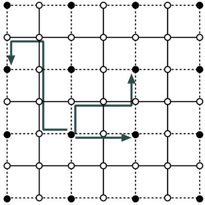
Figure 1: Two-grid decomposition of a two-dimensional lattice. Filled points are lattice sites of the coarse grid (${\cal L}_{1}$), open points sites of the fine grid (${\cal L}_{2}$). Dashed lines are links that enter in $M_{12}$ and $M_{21}$, while solid lines are those in $M_{22}$. The arrows show three possible contributions of order $2$, $4$, and $6$ to a general coarse-grid operator of the form (67).

III.2 Block $LU$ factorization

Eq. (16) and (17) can be expressed in matrix form as an block $LU$ decomposition of $M$. Its general form is

$$M=\left(\begin{array}[]{cc}1&-Q^{+}\\ 0&1\end{array}\right)\,\left(\begin{array}[]{cc}S&0\\ 0&T\end{array}\right)\,\left(\begin{array}[]{cc}1&0\\ -Q&1\end{array}\right)\quad.$$ (19)

The advantage of the representation (19) is that its inverse can be readily written as

$$M^{-1}=\left(\begin{array}[]{cc}1&0\\ Q&1\end{array}\right)\,\left(\begin{array}[]{cc}S^{-1}&0\\ 0&T^{-1}\end{array}\right)\,\left(\begin{array}[]{cc}1&Q^{+}\\ 0&1\end{array}\right)\,$$ (20)

requiring only the inversion of the smaller matrices $S$ and $Q$. In multigrid terminology, applying the factorization (20) to a vector amounts to first applying an restriction operator $Q^{+}$ that moves information from the fine grid to the coarse grid, then solving the effective coarse-grid operator $S$ along with the residual fine-grid operator $T$, and finally using the interpolation operator $Q$ to move information back from the coarse grid to the full grid.

Inserting (19) into (15) leads to the following relations that define $S$, $Q$, and $T$.

$$Sf_{1} = a_{1}-Q^{+}\,a_{2}\quad$$ (21)

$$T\left(-Qf_{1}+f_{2}\right) = a_{2}\quad.$$ (22)

Comparing with eq. (16) and (17) gives the solution

$$S = S_{M}=M_{11}-M_{12}M_{22}^{-1}M_{21}\quad,$$

$$Q = -M_{22}^{-1}M_{21}\quad,$$

$$T = M_{22}\quad.$$ (23)

The Schur complement is the exact effective coarse-grid operator associated with a given decomposition of the lattice. Unlike the geometrical approach, this decomposition is performed simply by thinning the matrix and thus without a block averaging that might introduce artifacts in the presence of a gauge field, and the resulting coarsened operator is defined solely in terms of the original matrix and thus the original disorder field. In the following sections, we will show that this procedure can be interpreted in terms of a noninteracting random walk leading to an explicit representation of the effective matrix in terms of a generalized path-dependent stencil.

III.3 Renormalization group and projective multigrid

The Schur complement has a close relation to the renormalization group approach used in statistical mechanics, where the Klein-Gordon and Dirac fields are described by a path integral with a Gaussian weight. In this approach, the partition sum

$$Z = \int{\rm d}f\,\exp\left[-\mbox{$\scriptstyle 1\over 2$}(f,Mf)+\mbox{$\scriptstyle 1\over 2$}(a,f)+{\rm c.c.}\right]$$

$$= \mbox{\rm const}\cdot e^{{\scriptstyle\frac{1}{4}}(a,M^{-1}a)}$$

(the integration is over all lattice field configurations $f$) generates the inverse of $M$ by taking the derivative with respect to the source field $a(x)$:

$$\left.\frac{1}{Z}\,\frac{\partial^{2}}{\partial a^{*}(x)\,\partial a(y)}\right|_{a=0}Z=\mbox{$\scriptstyle 1\over 2$}M^{-1}(x,y)\quad.$$ (24)

In renormalization-group inspired multigrid approach, such as proposed by Mack mack-1988 , Brower et. al. brower-edwards-rebbi-1991 or Vyas prd-vyas , one introduces new variables in the path integral by means of coarsening. In our terminology, a coarsened lattice field $F_{1}$ defined on on ${\cal L}_{1}$ is given by

$$F_{1}=f_{1}+Cf_{2}$$ (25)

where the coarsening matrix $C$ performs an averaging over neighboring sites in ${\cal L}_{2}$. (A more general coarsening would also include an averaging over neighboring sites from ${\cal L}_{1}$). The coarsened field $F_{1}$ is interpolated back to the fine lattice using an interpolation kernel $A$ and subtracted from $f_{2}$ to form the residual fine-grid field:

$$\zeta_{2}=f_{2}-AF_{1}$$ (26)

In this way, it is hoped that some of the dynamics of the fine lattice ${\cal L}_{2}$ is moved to the coarse lattice. The whole transformation reads

$$\left(\begin{array}[]{c}F_{1}\\ \zeta_{2}\end{array}\right)=\left(\begin{array}[]{cc}1&0\\ -A&1\end{array}\right)\,\left(\begin{array}[]{cc}1&C\\ 0&1\end{array}\right)\,\left(\begin{array}[]{c}f_{1}\\ f_{2}\end{array}\right)\quad.$$ (27)

As its determinant is unity, $F_{1}$ and $\zeta_{2}$ can be used as new integration variables in the path integral. The quadratic form in the exponential is then

$$\left(f,Mf\right) = \left(\begin{array}[]{c}F_{1}\\ \zeta_{2}\end{array}\right)^{+}\left(\begin{array}[]{cc}1&A^{+}\\ 0&1\end{array}\right)\,\tilde{M}\,\left(\begin{array}[]{cc}1&0\\ A&1\end{array}\right)\left(\begin{array}[]{c}F_{1}\\ \zeta_{2}\end{array}\right)^{+}$$ (36)

$$\tilde{M} = \left(\begin{array}[]{cc}1&0\\ -C^{+}&1\end{array}\right)\,M\,\left(\begin{array}[]{cc}1&-C\\ 0&1\end{array}\right)\quad,$$ (41)

and the coupling to the external fields

$$(a,f)=\left(\begin{array}[]{c}a_{1}+A^{+}a_{2}-A^{+}C^{+}a_{1}\\ a_{2}-C^{+}a_{1}\end{array}\right)^{+}\,\left(\begin{array}[]{c}F_{1}\\ \zeta_{2}\end{array}\right)^{+}\quad.$$ (46)

Algebraic multigrid does not use coarsening; the coarse lattice field is obtained by thinning out the original lattice and thus $F_{1}=f_{1}$, $C=0$ and $\tilde{M}=M$. Then the block $LU$ decomposition (19) tells us that we can make the quadratic form (36) block diagonal by choosing $A=-M_{22}^{-1}M_{21}$, in which case the partition sum factorizes into a coarse-grid and a fine-grid integral:

$$Z = \int{\rm d}f_{1}\,e^{-\mbox{$\scriptstyle 1\over 2$}(f_{1},S_{M}f_{1})+\mbox{$\scriptstyle 1\over 2$}(a_{1}+A^{+}a_{2},f_{1})+{\rm c.c.}}\cdot\int{\rm d}f_{2}\,e^{-\mbox{$\scriptstyle 1\over 2$}(f_{2},M_{22}f_{2})+\mbox{$\scriptstyle 1\over 2$}(a_{2},f_{2})+{\rm c.c.}}\quad.$$ (47)

The coarse scale dynamics is obtained by taking derivatives of $Z$ with respect to $a_{1}$ at $a_{2}=0$ and is therefore completely contained in the first integral, which is governed by $S_{M}$, the Schur complement. Thus the algebraic multigrid choice of the interpolation kernel $A$ can be characterized as that choice that leads to a complete decoupling of fine and coarse degrees of freedom, which makes integrating out the fine-grid degrees of freedom $\zeta_{2}$ trivial. Note that the Schur complement can be used to obtain effective fermions such as used in the blocked fermion approach to full QCD prd-lippert .

If a nonvanishing averaging kernel $C$ is used, one can achieve complete decoupling in the quadratic form by applying the Schur complement to the matrix $\tilde{M}$, but now $a_{1}$ also couples to $\zeta_{2}$ in the source term (46), and the integral over $\zeta_{2}$ results in a nontrivial contribution to the partition sum. This contribution is governed by $\tilde{M}_{22}^{-1}$, the propagator of the residual modes $\zeta_{2}$ on the fine lattice, which is given by

$$\tilde{M}_{22}=M_{22}-M_{21}C-C^{+}M_{12}+C^{+}M_{11}C\quad.$$ (48)

One therefore strives to choose an averaging kernel $C$ such that $\tilde{M}_{22}^{-1}$ is as local as possible, indicating that most of the (long-range) dynamics has been moved to the coarse-lattice field $F_{1}$.

The decoupling of coarse and fine modes was at the heart of Mack’s original multigrid proposal mack-1988 , which was inspired by constructive quantum field theory. It was already noticed by Brower, Rebbi, and Vicari prd-43-1965 that minimizing the coupling between coarse and fine modes amounts in spirit to algebraic multigrid, and using a similar reasoning, the form of the Schur complement is mentioned in eq. (12) of brower-edwards-rebbi-1991 by Brower, Edwards, and Rebbi. In practice, in the projective multigrid method the coarsening $C$ was chosen to localize $\tilde{M}_{22}^{-1}$ as much as possible, and the interpolation $A$ to maximize the decoupling between coarse and fine modes. An explicit method for calculating $A$ for a given $C$ is specified as idealized multigrid algorithm by Kalkreuter heplat-9304004 ; heplat-9408013 , and it can be verified that for a “lazy” coarsening kernel $C=0$, the resulting interpolation kernel has the form (III.2). The actual calculation for nontrivial $C$ is numerically infeasible as it requires the solution of a nonlinear equation at each coarse lattice site, so instead the ground-state of a block-truncated matrix was used for the kernels, leading to the method known as ground-state projection multigrid. The effective coarse-grid matrix was then approximated by a Galerkin choice using the rows of $A$ as a basis.

Using the algebraic multigrid choice of $C=0$, we cannot optimize the decay of $M_{22}^{-1}$. However, as there is no induced coupling of $a_{1}$ to the fine lattice field $\zeta_{2}$, the Schur complement provides an explicit representation of the complete coarse-lattice dynamics. In the following, we will discuss the interpretation of this quantity based on the diffusion representation.

III.4 Diffusion on a multigrid

In sec. II.2, the diffusion representation of the inverse of a matrix $M$ was introduced. The matrix elements of the Schur complement $S_{M}$ define a similar effective diffusion process involving only coarse lattice sites with transition probabilities and gauge phases determined by the elements of $S_{M}$. As $S_{M}^{-1}$ is identical with the upper left submatrix of $M^{-1}$,

$$S_{M}^{-1}(x,y)=M^{-1}(x,y)\qquad\mbox{for }x,y\in{\cal L}_{1}\quad,$$ (49)

this diffusion process is equivalent to the original diffusion process when origin and destination of the random walk are restricted to the coarse lattice. Using (18), the matrix elements of $S_{M}$ can itself be written in a diffusion representation:

$$S_{M}(x,y) = \delta_{x,y}-\sum_{n}\sum_{\begin{array}[]{c}(x,x_{1},\ldots,x_{n},y)\\ x_{1},\ldots,x_{n}\in{\cal L}_{2}\end{array}}\kappa^{n}\,{\cal P}(U;x,x_{1},\ldots,x_{n},y)\quad.$$ (52)

Since the sum comes from expanding $M_{22}^{-1}$, the inner parts $(x_{1},\ldots,x_{n})$ of the paths run exclusively on the fine lattice ${\cal L}_{2}$; they are connected to the coarse lattice ${\cal L}_{1}$ at points $x$ and $y$ through the matrix elements of $M_{12}$ and $M_{21}$ (some of these paths are shown in Fig. 1). The matrix elements of the Schur complement can therefore be interpreted as resulting from random walks on the fine complement lattice ${\cal L}_{2}$, and when the Schur complement is inverted, it defines a random walk on the coarse lattice ${\cal L}_{1}$, in each of whose steps all possible paths on the fine lattice ${\cal L}_{2}$ are effectively taken into account. In this way, the Schur complement allows to “integrate out” the fine degrees of freedom in the diffusion process much as renormalization group transformations do.

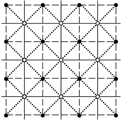
Figure 2: Two-grid decomposition of a odd-even decomposed lattice. As in Fig. 1, filled circles mark sites of the coarse grid, and open circles those of the fine grid. Full lines show links from $M_{22}$, dashed lines those from $M_{11}$, and dotted lines those from $M_{12}$. $M_{11}$ and $M_{22}$ here form two similar grids, with $M_{12}$ connecting the two along the diagonals.

In the two-dimensional case, the situation can be made more symmetrical by performing and even-odd-decomposition before the multigrid decomposition. In an even-odd decomposition, the matrix is replaced by the effective matrix on the even sites of the lattice,

$$S_{ee}=1-M_{eo}M_{oe}\quad,$$ (53)

where $M_{eo}$ and $M_{oe}$ are the matrix elements of $M$ between even and odd sites, resp. In the resulting lattice topology, each site is linked both to its four next neighbors in the straight direction as well to the four next neighbors in the diagonal (cf. Fig. 2). Applying now the multigrid decomposition, the lattice decomposes into two similar square lattices. $M_{11}$ and $M_{22}$ are represented by the straight links on each lattice, while $M_{12}$ and $M_{21}$ are carried by the diagonals linking the two lattices. The effective hopping parameter on each lattice is $\kappa_{\rm eff}=\frac{\kappa^{2}}{1-4\kappa^{2}}$ and thus smaller than on the original lattice, and consequently $M_{11}$ and $M_{22}$ are less critical than $M$. In the diffusion interpretation, even if probability was conserved on the original lattice, it is not conserved on the two sublattices individually, as the random walkers can move from one lattice to the other along the diagonal links represented by $M_{12}$ and $M_{21}$. The criticality of the system is only regained when $M_{11}$ and $M_{22}$ are combined in the Schur complement.

The propagator on the fine lattice $M_{22}^{-1}$ will therefore be short-ranged and can be incorporated approximately by considering only a limited number of hops on the fine lattice in the expansion (52). In the following section, we exploit this to construct an approximate Schur complement numerically.

IV Construction of the multigrid operator

The central problem in deriving a multigrid algorithm for disordered systems is the construction of a suitable approximation to the Schur complement $S_{M}$ and the block $LU$ decomposition (19).

IV.1 Numerically optimized Schur complement

Our method is based on numerically approximating the Schur complement as a linear combination of suitable basis operators. The full Schur complement $S$ usually cannot be computed exactly, but it can be characterized numerically by a sufficiently large set of pairs $\{f^{(n)},a^{(n)};n=1,\ldots,N\}$ which satisfy

$$M(U^{(n)})f^{(n)}=a^{(n)}\quad,$$ (54)

where it is explicitly indicated that $M$ depends on different realizations $U^{(n)}$ of the disorder field. Using the block $LU$ decomposition (19), this implies that $S$, $Q$, and $T$ satisfy the relations (21), (22). In particular, if the pairs are chosen such that $a_{2}=0$, their coarse-lattice components $\{f_{1}^{(n)},a_{1}^{(n)}\}$ characterize the Schur complement by the relation:

$$Sf_{1}^{(n)}=a_{1}^{(n)}\quad.$$ (55)

Similarly, the interpolation operator is characterized by the pairs $\{f_{1}^{(n)},f_{2}^{(n)}\}$ using

$$Qf_{1}^{(n)}=f_{2}^{(n)}\quad.$$ (56)

There is no need to approximate $T=M_{22}$, as it does not contain the inverse of $M_{22}$. An approximation $\bar{S}$ to $S$, and similarly $\bar{Q}$ to Q, can then be characterized with minimum bias by the mean error norm of (55):

$$\delta^{2}=\sum_{n}^{N}\left|\bar{S}(U^{(n)})f_{1}^{(n)}-a_{1}^{(n)}\right|^{2}$$ (57)

This quantity is an approximation to an operator norm $|\bar{S}S-1|^{2}$ averaged over gauge field configurations. The choice of pairs (54) introduces a weight function in this norm and thus determines which functions are well approximated by $\bar{S}$. Eq. (57) can be rewritten as

$$\delta^{2}=\sum_{n}^{N}\left|\left(\bar{S}(U^{(n)})S-1\right)a_{1}^{(n)}\right|^{2}=\sum_{n}^{N}\left|\left(\bar{S}(U^{(n)}-S(U^{(n)}\right)f_{1}^{(n)}\right|^{2}$$ (58)

If $f_{1}$ is chosen randomly on the whole function space, $\delta^{2}$ thus approximates $|\bar{S}-S|^{2}$, while if $a_{1}$ is chosen randomly, it approximates

$$|\bar{S}S^{-1}-1|^{2}=|(\bar{S}-S)S^{-1}|^{2}$$ (59)

The factor $S^{-1}$ increases the weight of functions that have eigenvalues closer to zero, and these are exactly the long-ranged functions we are interested in. Choosing the right-hand sides $a_{1}$ also allows us to enforce $a_{2}=0$ and thus remove $Q$ from the (21). In practice, we choose $a$ to be a delta function on a randomly chosen coarse-lattice point, and determine $f$ by solving the linear system (54). In other words, the $f^{(n)}$ are Green’s functions, or propagators in lattice gauge theory language, and we look for an approximate operator $\bar{S}$ that well reproduces the action of $S$ on these functions.

If we choose a general linear combination of suitably chosen basis operators $S^{(i)}(U)$ respecting the symmetries of the problem as approximate operators,

$$\bar{S}(U)=\sum_{i}\alpha_{i}\bar{S}^{(i)}(U)\quad,$$ (60)

the approximation error $\delta^{2}$ is a quadratic form in the coefficients $\alpha_{i}$:

$$\delta^{2} = \sum_{ij}\alpha_{i}^{\ast}\,A_{ij}\,\alpha_{j}-\sum_{i}\alpha_{i}\,B_{i}^{*}-{\rm c.c.}+C$$ (61)

$$A_{ij} = \sum_{n}^{N}\,\left(S^{(i)}(U^{(n)})f_{1}^{(n)},S^{(j)}(U^{(n)})f_{1}^{(n)}\right)_{{\cal L}_{1}}$$ (62)

$$B_{i} = \sum_{n}^{N}\,\left(S^{(i)}(U^{(n)})f_{1}^{(n)},a_{1}^{(n)}\right)_{{\cal L}_{1}}$$ (63)

$$C = \sum_{n}^{N}\,\left(a_{1}^{(n)},a_{1}^{(n)}\right)_{{\cal L}_{1}}$$ (64)

where $(a_{1},b_{1})_{{\cal L}_{1}}$ denotes that scalar product on the coarse grid ${\cal L}_{1}$. Thus the minimum of the approximation error and thus the optimal choice of coefficients is found simply by:

$$\alpha_{i}=\sum_{j}(A^{-1})_{ij}B_{j}$$ (65)

The procedure for finding the coefficients of the numerical approximation to the Schur complement is therefore as follows:

1. Generate right-hand sides $a^{(n)}$ by choosing random delta functions on the coarse grid.

2. Find the corresponding $f^{(n)}$ by solving (54) using the original fine-grid operator $M$.

3. Project $a^{(n)}$ and $f^{(n)}$ to the coarse lattice.

4. Calculate the matrix elements (62) and (63) and find $\alpha_{i}$ from (65).

A similar procedure is used to approximate the interpolation operator $Q$. This method is similar to Monte Carlo renormalization group as it calculates the coefficients of the effective coarse-grid operator by applying a block-spin transformation (in our case, simply a projection) to an ensemble of configurations on the fine grid. Note that the procedure is completely general and can be used to approximate any operator, e.g. the Neuberger or a renormalization-group improved operator, if its action on some sample fields is known.

IV.2 Choice of the operator basis

The approximate coarse-grid operator $\bar{S}(U)$ is a general operator-valued function of the disorder field $U$, but the symmetries of the problem greatly restrict the possible basis operators $\bar{S}^{(i)}(U)$ from which it can be constructed. To maintain gauge covariance, each contribution to the matrix element $M(x,y)$ can be factored into a gauge-field independent part and a product of the gauge field links along a connected path from $x$ to $y$, leading to the following representation of $M$:

$$M(x,y)=\sum_{n}\sum_{P=(\mu_{1},\ldots,\mu_{n})}\,m(P)\,\delta_{y,x+e_{\mu_{1}}+\cdots+e_{\mu_{n}}}\,{\cal P}_{\mu_{1},\ldots,\mu_{n}}(U;x)$$ (66)

where the sum is over connected paths from $x$ to $y$, and the reduced matrix element $m(P)$ does not depend on the gauge field $U$. Basis operators $S^{(i)}$ can thus be associated with the possible relative paths $P_{i}=\{\mu_{1},\ldots,\mu_{n}\}$:

$$\bar{S}^{(i)}(U)(x,y)=\Gamma^{(i)}\delta_{y,x+\mu_{1}+\cdots+\mu_{n}}\,{\cal P}_{\mu_{1},\ldots,\mu_{n}}(U;x)\quad,$$ (67)

where $\Gamma^{(i)}$ is independent of $x$, $y$, and $U$, and serves to contain a possible internal structure of the field, e.g. the Dirac $\gamma$ matrices.

Other symmetries like translation, rotation, and reflection invariance as well as hermiticity and charge conjugation generate further restrictions on the coefficients $\alpha_{i}$. In the calculations, our computer code automatically evaluates discrete rotation and reflection symmetry for all paths and constructs basis operators that are invariant under these transformations. This reduces significantly the number of degrees of freedom in (61). Hermiticity places constraints on the real and imaginary parts of the coefficients; it is not enforced and can be used as a check of the accuracy of the constructed operator. The general problem of constructing generalized Dirac operators was recently brought up in the context of chirally-enhanced operators in heplat-0001001 ; heplat-0003005 and discussed in general in heplat-0003013 .

The representation (66) has the same form as the diffusion representation (52), with the additional restriction that only paths moving exclusively on the fine lattice contribute there. The optimization process (57) thus results in assigning weights to the different paths in the diffusion representation that reflect how much a path contributes, on average, to the propagator. If a complete sum over all lengths $n$ is taken, the correct weights are of course $\kappa^{-n}$, as in the von Neumann series. However, if the sum is truncated, the weights are modified in the optimization process and the contributions of the individual paths renormalized to take the obmitted paths into account.

The basis (67) can be compared to the situation without a gauge field. In the terminology of numerical analysis, a translation-invariant operator is represented by a stencil $S(a)$ using the expression corresponding to (66)

$$M(x,y)=\sum_{a}S(a)\,\delta_{y,x+a}$$ (68)

where $a$ runs over the possible offsets between lattice points. The basis operators in this case can therefore be labeled by the offset $a$, and the equation corresponding to (67) reads

$$S^{(i)}(x,y)=\delta_{y,x+a_{i}}\quad.$$ (69)

Comparing the two cases, one can see that in the disordered case the relative paths take over the role of the offsets, and a generalized stencil is given by assigning each relative path a certain weight. The optimization procedure corresponds to calculating such a generalized stencil, much as an ordinary stencil is constructed for differential equations.

Once the disordered stencil is known, the coarse-grid operator $S$ for any gauge field can be constructed simply by evaluating all paths in the set $\{S^{(i)}\}$ and combining them according to the weights $\alpha_{i}$. Note that it is not necessary to perform the construction of the on the actual set of gauge fields, but on a representative ensemble only, so the optimization can be performed in advance of the simulation.

The resulting coarse-grid operator contains in particular also contributions beyond direct neighbors on the coarse grid, similar to improved and perfect operators that lose locality but gain a more faithful representation of the continuum operator, and the amount of nonlocality can be tuned by selecting the paths in the basis set. On the other hand, if the basis set is chosen to reproduce the original topology on the coarse lattice, the coarse-grid operator defines a new effective disorder field on the coarse-grid. However, this disorder field is obtained by a sum and will therefore lie outside the gauge group, though it can be projected back to the gauge group, as is customarily done in many renormalization schemes. In this way, the Schur complement can be used to define a block-spin transformation for the gauge field.

IV.3 Construction in the diagonal subspace

The basis (67) is the most general set of operators that can make up a gauge-covariant operator. Its size grows exponentially with the order of the path set and thus makes both the evaluation of the coefficients (62) and (63) and the actual construction of the approximate Schur complement very time consuming. A smaller and thus more tractable basis can be found by considering the operators that appear in the von Neumann series (II.2) which are:

$$\bar{S}^{(0)} = M_{11}\quad,$$

$$\bar{S}^{(i+1)} = M_{12}M_{22}^{2i}M_{21}\quad.$$ (70)

This basis generates exactly the same paths as the diffusion representation (67) restricted to the fine lattice, but uses coefficients that only depend on the length of the paths. Obviously, if an infinite set of basis operators is used, the optimal coefficients are $\pm 1$ as given by the von Neumann series. However, in a finite set, the optimization procedure amounts to finding a polynomial approximation to the inverse function.

To see this, let $T$ be an approximation to $M_{22}^{-1}$, and write the approximate Schur complement as

$$\bar{S}=M_{11}-M_{12}TM_{21}$$ (71)

Inserting this into (57) gives after some algebra

$$\left|\bar{S}f_{1}-a_{1}\right|^{2}=\left(T\hat{f},M_{21}M_{12}T\hat{f}\right)_{2}-2\Re\left(\hat{b},T\hat{f}\right)_{2}+\left(b,b\right)_{1}$$ (72)

with the notation $(\ldots,\ldots)_{2}$ for the scalar product over ${\cal L}_{2}$ and the definitions

$$\hat{f} = M_{21}f_{1}\quad,$$ (73)

$$b = M_{11}f_{1}-a_{1}\quad,$$

$$\hat{b} = M_{21}b$$ (74)

$$= M_{21}M_{12}M_{22}^{-1}M_{21}f_{1}\quad,$$

where we used (55) and (18) in the last line. If $T$ is a polynomial in $M_{22}$, it is diagonal in the eigenbasis of $M_{22}$ and can be written as

$$M_{22} = \sum_{k}\lambda_{k}\,v_{k}\otimes v_{k}^{+}$$ (75)

$$T = \sum_{k}T_{k}\,v_{k}\otimes v_{k}^{+}$$ (76)

where $\lambda_{k}$, $v_{k}$ are eigenvalues and -vectors of $M_{22}$, and $T_{k}$ the diagonal elements of $T$ in the eigenrepresentation. Inserting this into (72) gives the following quadratic form for the diagonal components $T_{k}$ of the operator $T$:

$$\left|\bar{S}f_{1}-a_{1}\right|^{2} = \sum_{kl}T_{k}^{\star}\,(\hat{f}^{\star}_{k}\hat{f}_{l})\,\left(M_{21}M_{12}\right)_{kl}T_{l}$$ (78)

$$-2\Re\sum_{k}T_{k}\,(\hat{b}^{\star}_{k}\hat{f}_{k})+\mbox{\rm const}$$

where $\hat{f}_{k}=(v_{k},\hat{f})$, $\hat{b}_{k}=(v_{k},\hat{b})$ are the representations of $\hat{f}$ and $\hat{b}$ in the eigenspace of $M_{22}$, and similarly for $(M_{21}M_{12})_{kl}$. Eq. (74) relates these quantities by

$$\hat{b}_{k}=\sum_{l}(M_{21}M_{12})_{kl}\,\lambda_{l}^{-1}\,\hat{f}_{l}$$ (79)

which gives the following expression for (78):

$$\left|\bar{S}f_{1}-a_{1}\right|^{2} = \sum_{kl}\left(T_{k}-\frac{1}{\lambda_{k}}\right)^{\star}\,(\hat{f}^{\star}_{k}\hat{f}_{l})\,\left(M_{21}M_{12}\right)_{kl}\,\left(T_{l}-\frac{1}{\lambda_{l}}\right)+\mbox{\rm const}$$ (80)

$$= \sum_{k}\left|\sum_{l}\left(M_{12}\right)_{kl}\hat{f}_{l}\,\left(T_{l}-\frac{1}{\lambda_{l}}\right)\right|^{2}+\mbox{\rm const}\quad.$$

Minimizing this quantity thus amounts to finding a best approximation $T_{k}$ to $\lambda_{k}^{-1}$ in a weighted square norm specified by $M_{12}\hat{f}=M_{12}M_{21}f_{1}$.

Choosing for $T$ a polynomial form

$$T=\sum_{n=0}^{N}\alpha_{n+1}\,M_{22}^{2n}\qquad,\quad T_{k}=\sum_{n=0}^{N}\alpha_{n+1}\,\lambda_{k}^{2n}$$ (81)

in accordance with the expansion (IV.3), the approximate Schur complement then takes the form

$$\bar{S}=M_{11}-\sum_{k=0}^{N}\alpha_{k+1}M_{12}M_{22}^{2k}M_{21}$$ (82)

Fig. 3 shows a numerical evaluation of such an approximation using the Dirac operator on a sample $U(1)$ configuration.

An operator of the form (82) can be computed relatively easily: The coefficient $\bar{S}(x,y)$ between two sites is given by summing the phase factors over all paths from $x$ to $y$ on ${\cal L}_{2}$ with weights depending only on the length of the paths and given by the coefficients $\alpha_{k}$. This is a simplification over the full path set (67), where each path can be assigned its own weight. If only a finite number $N$ of coefficients is used, the operator is local, but contains more than next-neighbor interactions. Note that in a typical iteration scheme the calculation of the matrix elements of $\bar{S}$ has to be done only once, and the complexity of the iteration depends only on the sparsity of the resulting $\bar{S}$.

Figure 3: Numerical evaluation of the optimal polynomial approximation to $M_{22}^{-1}$. The curves show the polynomial approximations of order 1, 3, 5, and 7 to the inverse function. The actual eigenvalues are marked with crosses.

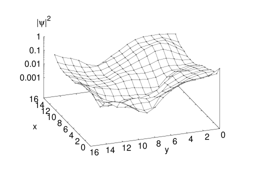
Figure 4: Absolute value of a sample fermionic Green’s function on an $16\times 16$ lattice in a $U(1)$ background field for the original Dirac operator (left) and the approximate coarse-grid operator obtained from the Schur complement. The source is located at the origin; since the lattice is periodic, it shows up at the four corners of the plot.

Figure 5: Cut through the example fermionic Green’s function (black squares) compared to Green’s functions calculated from an approximate Schur complement and interpolation operator of order 1, 2, and 4.

IV.4 Numerical results

We have numerically evaluated the optimal operator both for the full path set of eq. (67) and the subset defined in eq. (IV.3). The calculations were performed for the Dirac equation on a $16\times 16$ lattice in two dimensions in a $U(1)$ gauge field generated at $\beta=3.0$, which results in relatively smooth configurations and long-ranged correlation functions. Fig. 5 and 5 show sample Green’s functions of the original Dirac matrix and the approximate Schur complement. The disorder from the gauge field shows up clearly in the Green’s function, but the various approximations to the Schur complement reproduce the irregularities and the overall form of the function quite well.

Figure 6: The relative approximation error as a function of the order of the approximation, calculated in an ensemble of 10 independent $16\times 16$ $U(1)$ gauge configurations at $\beta=3.0$ and $\kappa=0.265$. The full line gives the result from the optimization in the diagonal subspace, the dashed line from the full optimization. The dotted line is the relative error of the truncated von Neumann series of the same order.

Figure 7: The relative inversion error as a function of the approximation order for both diagonal and full optimization. For comparison, the original relative error from Fig. 7 is also shown.

This is quantified in fig. 7, which shows the average relative error

$$\sqrt{\frac{\delta^{2}}{\sum_{n}^{N}|a_{1}^{(n)}|^{2}}}$$ (83)

evaluated in an ensemble of ten sample $U(1)$ gauge configurations generated at $\beta=3.0$ on a $16\times 16$-lattice. For each configuration, five different Green’s function at $\kappa=0.265$ on each configuration were calculated and the coefficients (62) and (63) that characterize the error ellipsoid were evaluated. For the diagonal optimization, the basis (IV.3) with maximum order $i$ from $1$ to $6$, corresponding to a maximum path length from $2$ to $12$, was used. For the full optimization, a complete path basis of paths up to length $2i$ constrained to the discrete rotation and reflection symmetry was taken. For comparison, the relative error resulting from the von Neumann series is also shown. The errors show a very clean logarithmic dependence on the order. As the number of paths in the operator increases exponentially with order, this corresponds to a polynomial dependence of the error on the number of paths.

The full path set gives only a slightly better approximation than the diagonal approximation, though it is significantly more difficult to evaluate, as the number of coefficients grows exponentially. Its main advantage is that it allows to fine-tune the number and characteristics of the paths, e.g. the maximum distance between end points. Fig. 7 shows the resulting errors when the error ellipsoid is restricted to a certain number of paths. It turns out that the relative error has a power law dependence on the number of paths, with an exponent of approximately $-0.55$ in this case. The contributions from different operators are relatively uniform except for the operators in the tails that contribute little or nothing, so the accuracy of the approximate Schur complement can be fine-tuned by varying the number of paths in the operator.

The relative error measures how well the approximate Schur complement reproduces a delta function when applied to a Green’s function. For actual applications, the more relevant quantity is the relative inversion error that looks at how good the inverse of the approximate Schur complement reproduces the Green’s function of the original matrix. This is quantified by

$$\delta_{\rm inv.}^{2}=\sum_{n}^{N}\left|\bar{f}_{1}^{(n)}-S^{-1}(U^{(n)})a_{1}^{(n)}\right|^{2}$$ (84)

with the relative error taken relative to the norm of $f_{1}^{(n)}$: This quantity was evaluated numerically by computing Green’s function of the approximate Schur complement on the coarse lattice and comparing the results to the Green’s functions of the original Wilson-Dirac matrix. Fig. 7 shows the relative error as a function of the approximation order both for the diagonal and the full optimization. It also decreases exponentially but is about twice the magnitude of the original error.

IV.5 Spectrum

The low eigenvalues of the original matrix $M$ have a direct relation to those of the Schur complement $S_{M}$. If $f$ is an eigenvector of $M$ with eigenvalue $\lambda$,

$$Mf=\lambda f\quad,$$ (85)

this becomes using (16)

$$Sf_{1} = \lambda f_{1}-M_{21}M_{22}^{-1}\,\lambda f_{2}$$

$$M_{22}f_{2} = \lambda f_{2}-M_{21}f_{1}\quad.$$ (86)

Eliminating $f_{2}$ in the first line yields a modified eigenvalue equation for $S$:

$$Sf_{1}=\lambda\,\left(1+M_{12}M_{22}^{-1}(M_{22}-\lambda)^{-1}M_{21}\right)\,f_{1}\quad.$$ (87)

If the eigenvalues of $M_{22}$ are large, as argued in sec. III.4, the additional term on the right-hand side multiplying the eigenvalue is approximately

$$1+M_{12}M_{22}^{-2}M_{21}=1+Q^{+}Q\quad.$$ (88)

Assuming further that $M_{22}^{-1}$ is short-ranged, the second term can be approximated by a constant $\alpha$ when acting on a low eigenvector, and (87) becomes

$$Sf_{1}\approx\lambda(1+\alpha)f_{1}\quad.$$ (89)

This rescaling of the eigenvalues accounts for the different lattice constant of the coarse grid. The appearance of the interpolation kernel $Q$ in (88) shows that it accounts for the parts of the original eigenvector that were on the fine grid and therefore dropped. In a geometric multigrid method, this is usually done by the coarsening prescription which moves information from fine to coarse degrees of freedom; in algebraic multigrid, it results directly from the $LU$ decomposition.

Fig. 10 shows the lowest positive eigenvalues of the Dirac matrix and different forms of the Schur complement for a sample $U(1)$ gauge configuration at $\beta=3.0$. With a rescaling factor of approximately $1+\alpha\approx 4$, the exact Schur complement $S_{M}$ reproduces the low eigenvalues of $M$ well, and so does the order-2 optimized operator. The truncated von Neumann series, however, deviates significantly from the true results for the lowest eigenvalues, which are expected to be very important for the convergence properties when used as a preconditioner.

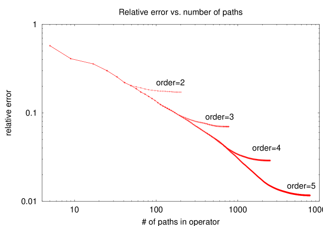
Figure 8: The relative error as a function of the number of paths in the approximate Schur complement for different orders of the path set. The paths have been reordered so that the relative error decays fastests.

Figure 9: The relative error from the full optimization as a function of the maximum distance of path end points in the path set, shown for different maximum lengths of the path.

Figure 10: Lowest positive eigenvalues of the effective coarse-grid operator $S$. The lower curve (filled circles) shows eigenvalues of the full Dirac matrix on a $16\times 16$ lattice with a sample $U(1)$ gauge field at $\beta=3.0$. The three upper curves are the corresponding eigenvalues on the coarse grid, calculated from the exact Schur complement (full squares), the order-2 optimized operator (open squares), and the order-2 von Neumann series (open diamonds). The inset enlarges low eigenvalues.

V Applications

While a full discussion of the performance of multigrid operators in different algorithms is outside of the scope of this paper, we give here two examples of how they can be applied in numerical algorithms. Preconditioning uses the block $LU$ decomposition provided by the multigrid decomposition to improve the condition number and thus convergence in iterative algorithms. Multigrid relaxation is the classical multigrid algorithm for solving the system (14) and allows a comparison between a two-grid iteration and the original fine-grid iteration. In all calculations, a $16\times 16$ lattice was used to allow the calculation of complete spectra. Note that only two-grid algorithms are considered; for realistic problems, the procedure should be repeated on several grid levels.

Figure 11: Spectra of the multigrid preconditioned Dirac matrix $1-\bar{M}^{-1}M$ for a sample gauge field configuration. Optimized approximations of order 1, 2, and 3 where used from left to right for the Schur complement. The top row shows the spectra obtained using an approximate interpolation operator, the bottom row the spectra using the exact interpolation operator. Preconditioning with an exact Schur complement and interpolation operator would result in a single point at the origin.

Figure 12: The preconditioned spectrum of fig. 12, using the von Neumann series as approximate Schur complement.

V.1 Preconditioning

In preconditioning, the linear system

$$Mf=a$$ (90)

is replaced by an equivalent system

$$\bar{M}^{-1}Mf=a^{\prime}=\bar{M}^{-1}a$$ (91)

using a preconditioning matrix $\bar{M}$ that is an easily invertible approximation to $M$. If $\bar{M}$ is sufficiently close to $M$, the spectrum of the preconditioned matrix $\bar{M}^{-1}M$ is contracted towards unity and its condition number reduced. For multigrid preconditioning, one uses an approximate block LU decomposition of the form (19) as the preconditioner. The preconditioned matrix is then

$$\bar{M}^{-1}M=\left(\begin{array}[]{cc}1&0\\ \bar{Q}&1\end{array}\right)\,\left(\begin{array}[]{cc}\bar{S}^{-1}&0\\ 0&\bar{T}^{-1}\end{array}\right)\,\left(\begin{array}[]{cc}1&\bar{Q}^{+}\\ 0&1\end{array}\right)\,\left(\begin{array}[]{cc}M_{11}&M_{12}\\ M_{21}&\bar{M}_{22}\end{array}\right)$$ (100)

If $Q$ and $T$ are chosen to be exact, $Q=-M_{22}^{-1}M_{21}$ and $T=M_{22}$, this reduces to

$$\bar{M}^{-1}M=\left(\begin{array}[]{cc}\bar{S}^{-1}S_{M}&0\\ \bar{Q}\bar{S}^{-1}(\bar{S}^{-1}S_{M}-1)&1\end{array}\right)\quad.$$ (101)

The properties of the preconditioner are therefore determined by $1-\bar{S}^{-1}S_{M}$, which is the quantity that was optimized in the optimization process (59) above.

Fig. 12 shows sample spectra of $1-\bar{M}^{-1}M$ with the Schur complement approximated to order 1, 2, and 3. If an exact Schur complement was used, the spectrum would reduce to a single point at the origin; the radius of the disk on which the eigenvalues lie in the complex plane is a measure of the quality of the preconditioner. The figure shows the result for two different choices of the interpolation matrix $Q$: In the bottom row, the exact interpolation $Q=-M_{22}^{-1}M_{21}$ was used. Since $Q$ is, as opposed to $S$, never inverted in the process, this is numerically legitimate and no more complex than the application of the approximate $S^{-1}$. The top row shows the result when an approximate interpolation matrix $\bar{Q}$ was used that was calculated in the same way as $S$ in an optimization process. It shows that only if a high order of approximation for $S$ was chosen, it makes sense to use the exact interpolation operator, otherwise it just leads to a larger concentration of eigenvalues without reducing the radius of the disk.

For comparison, fig. 12 shows the spectrum of a matrix that was preconditioned using von Neumann series (and the exact interpolation operator) to the same order as before. While most modes are quite well reduced, there remain even at order 3 a few eigenvalues far away from the origin. These probably correspond to low eigenvalues of the original matrix that are not properly approximated by the von Neumann series, as seen in fig. 10 above.

Figure 13: Spectra of the convergence matrix for multigrid relaxation in a sample gauge field. Optimized approximations of order 1, 2, and 3 where used from left to right for the Schur complement. The top row shows the convergence of the multigrid cycle if a full inversion is performed on the coarse grid, and one relaxation step on the fine grid. The bottom row shows the same spectrum if only a single relaxation step is performed on each grid. The convergence rate is given by the radius of the smallest disk containing eigenvalues.

V.2 Multigrid relaxation

Relaxation schemes for solving eq. (14) make use of an iterative process with an update step that is derived from the residual

$$r^{(n)}=a-Mf^{(n)}\quad,$$ (102)

where $f^{(n)}$ is the current approximate solution. The true error, i.e. the amount by which $f^{(n)}$ has to be updated, can be calculated from the residual by

$$e^{(n)}=f-f^{(n)}=M^{-1}r^{(n)}\quad.$$ (103)

Given an approximation $\bar{M}^{-1}$ to $M^{-1}$, an approximate update step reads

$$f^{(n+1)}=f^{(n)}+Tr^{(n)}=(1-\bar{M}^{-1}M)f^{(n)}+Ta\quad.$$ (104)

This iteration always has a fixed point at the true solution $f$, and the quality of the approximation $\bar{M}^{-1}$ to $M^{-1}$ only determines the convergence characteristics of the process.

Multigrid relaxation is based on using the Schur complement along with restriction and interpolation to construct an approximation to $M^{-1}$ on the coarse lattice. First, the residual is restricted to the coarse lattice using the restriction

$$\bar{r}^{(n)}=e_{1}+Q^{+}e_{2}\quad.$$ (105)

A coarse lattice approximation $\bar{e}^{(n)}$ to the true error is then found by applying the inverse of the approximate Schur complement:

$$\bar{e}^{(n)}=\bar{S}^{-1}\bar{r}^{(n)}\quad.$$ (106)

Finally, this is interpolated back to the fine lattice:

$$\bar{e}_{1}^{(n)}=\bar{e}^{(n)}\quad,\qquad\bar{e}_{2}^{(n)}=Q\bar{e}^{(n)}$$ (107)

and used to update the approximation. This update step acts on the coarse degrees of freedom only and must be followed by a compatible relaxation step on the fine lattice. In matrix form, the approximate inverse of $M$ used here reads

$$T=\left(\begin{array}[]{cc}1&0\\ \bar{Q}&1\end{array}\right)\,\left(\begin{array}[]{cc}\bar{S}^{-1}&0\\ 0&0\end{array}\right)\,\left(\begin{array}[]{cc}1&\bar{Q}\\ 0&1\end{array}\right)\quad.$$ (108)

It differs from the true LU decomposition (20) in that the lower right entry of the matrix in the middle is zero instead of $M^{-1}_{22}$. If a perfect interpolation and restriction is chosen, $\bar{Q}=-M_{22}^{-1}M_{21}$, the iteration matrix for the coarse-grid step reads

$$1-TM=\left(\begin{array}[]{cc}1-\bar{S}^{-1}S&0\\ Q\bar{S}^{-1}S&1\end{array}\right)\quad.$$ (109)

Its convergence properties on the coarse lattice are thus given again by $1-\bar{S}^{-1}S$ as in the case of preconditioning; on the fine lattice, it performs no relaxation at all, and must be followed by an ordinary relaxation step using $M_{22}$.

Figure 14: Sample convergence of a two-grid relaxation method compared to the same method applied to the base grid, for a $U(1)$ Dirac operator on a $16\times 16$-lattice. The horizontal axis gives the number of floating-point multiplications, the vertical axis the true error of the algorithm. For the two-grid algorithm, one sweep on the coarse lattice and one sweep on the fine lattice were performed alternately.

Fig. 13 shows the spectra of the convergence matrix for multigrid relaxation. In the top row, each step consists of performing a complete relaxation on the coarse lattice, and one relaxation step on the fine lattice. This leads to a concentration of eigenvalues around zero, showing modes that are nearly completely reduced on the coarse grid. The remaining modes must be reduced on the fine grid and determine the residual convergence rate. In an actual application, one would not completely reduce the modes on the coarse grid, but perform coarse- and fine-grid relaxation alternately. The resulting convergence spectrum is shown in the bottom row; it has a similar convergence rate as the complete reduction, but requires much less operations. Note that increasing the order of the approximation from 2 to 3 does not improve the convergence, but this might be related to the fact that only one fine-grid relaxation step was used here.

Finally, we compare the number of operations required to calculate a sample Green’s function in $U(1)$ lattice gauge theory on a $16\times 16$ lattice. It must be cautioned that this is only an example calculation using two-grid relaxation, not a full multigrid algorithm. The method offers a multitude of choices and tunable parameters: the order and type of the approximation for the $LU$ decomposition, the iterative algorithm (used here is for simplicity Jacobi relaxation; in actual applications one would probable use Gauss-Seidel), the multigrid cycle, and the convergence criteria on the two grids. The size and dimensionality of the lattice and the gauge group, as well as the amount of disorder in the gauge field, have been seen to decisively influence results in other algorithms. Also, the two-grid algorithm must be extended to a true multigrid algorithm by recursively applying the method. And finally relaxation might be less performant than a preconditioned Krylov solver. The ultimate measure of performance will be the actual computer time used in the algorithms, but this will depend on the implementation and on the architecture of the target machine. For example, the computation of the approximate Schur complement can either be performed beforehand and stored in memory, or on the fly in the matrix-vector multiplication of the Schur complement, depending on the amount of memory available. Here a lower order of approximation, resulting in a smaller Schur complement, can be favorable though its convergence rate per relaxation step might be slower.

With these precautions, an example run for calculating a sample Green’s function is shown in Fig. 14. As a measure of computer time used, the approximate number of floating-point multiplications is given. The convergence is measured as the error norm against the true result.

VI Conclusions

It was demonstrated how the algebraic multigrid method can be applied to disordered linear operators. Other than in previous multigrid approaches, a thinned lattice for the coarse degrees of freedom is used and averaging over block spins is avoided. The interpolation operator is chosen to obtain a block $LU$ decomposition, and the resulting coarse-grid dynamics is completely described by the Schur complement of the original matrix. Gauge covariance is automatically taken into account by this procedure.

The Schur complement can be approximated to arbitrary precision in a numerical optimization process by expanding it in a linear basis constructed from connected paths on the original lattice, forming a generalized stencil for disordered operators. Similar to renormalization group techniques, the numerical procedure for obtaining the expansion coefficients uses the coarse-grid projection of an ensemble of systems to obtain the coefficients of the approximate coarse-grid operator. In this way, the information gathered in the optimization process can be used to speed up the actual calculations as the optimized effective coarse-grid operator “learns” the dynamics of the system.

The resulting effective coarse-grid operator is constructed from the generalized stencil as a weighted sum over paths on the original lattice. It forms a denser, but smaller matrix with next-neighbor and higher interactions and can be used to improve performance in numerical algorithms by preconditioning or similar methods, hopefully not only for matrix inversion, but also for other problems such as eigensystem analysis and rational matrix functions. A variety of tunable parameters make it possible to adapt the procedure to different algorithms and architectures. Whether the method will actually improve real-life algorithms, remains of course to be seen until realistic systems and efficient implementations are investigated.

Acknowledgements
The author wishes to thank K. Schilling, T. Lippert, B. Medeke, and J. Negele for useful discussions, and the Center for Theoretical Physics at MIT for its hospitality. Computer time was provided by the NICse cluster computer at the John von Neumann Institute.

References

- (1) A. Frommer, V. Hannemann, B. Nöckel, T. Lippert, and K. Schilling, Accelerating the wilson fermion matrix inversions by means of the stabilized biconjugate gradient algorithm, Intl. J. Mod. Phys. C 5, 1073 (1994), eprint hep-lat/9404013.
- (2) A. Frommer, Linear systems solvers - recent developments and implications for lattice computations, Nucl. Phys. (Proc. Suppl.) 53, 120 (1997), eprint hep-lat/9608074.
- (3) M. H. Gutknecht, On Lanczos-type methods for Wilson fermions, in Frommer et al. wuppertal-1999-proceedings .
- (4) S. Fischer, A. Frommer, U. Glässner, T. Lippert, G. Ritzenhöfer, and K. Schilling, A parallel SSOR preconditioner for lattice QCD, Comp. Phys. Comm. 98, 20 (1998), eprint hep-lat/9602019.
- (5) M. Peardon, Accelerating the Hybrid Monte Carlo algorithm with ILU preconditioning (2000), eprint hep-lat/0011080.
- (6) W. Hackbusch, Multi-Grid Methods and Applications, no. 4 in Springer Series in Computational Mathematics (Springer, Berlin, 1985).
- (7) S. F. McCormick, ed., Multigrid Methods (SIAM, Philadelphia, 1987).
- (8) G. Mack, Multigrid methods in quantum field theory, in Nonperturbative Quantum Field Theory, edited by G. ’t Hooft et al. (Plenum Press, New York, 1988).
- (9) H. J. Herrmann and F. Karsch, eds., Workshop on Fermion Algorithms (World Scientific, Singapore, 1991).
- (10) R. C. Brower, C. Rebbi, and E. Vicari, Projective multigrid for propagators in lattice gauge theory, Phys. Rev. D 43, 1965 (1991).
- (11) R. C. Brower, K. J. M. Moriarty, C. Rebbi, and E. Vicari, Multigrid propagators in the presence of disordered gauge fields, Phys. Rev. D 43(6), 1974 (1991).
- (12) R. C. Brower, R. G. Edwards, C. Rebbi, and E. Vicari, Projective multigrid for wilson fermions, Nucl. Phys. B 366, 689 (1991).
- (13) V. Vyas, Calculating the quark propagator using the Migdal-Kadanoff transformation, in Herrmann and Karsch juelich-1991 , pp. 169–172.
- (14) V. Vyas, Real-space renormalization-group approach to the multigrid method, Phys. Rev. D 43(10), 3465 (1991).
- (15) R. Ben-Av, A. Brandt, M. Harmatz, E. Katznelson, P. G. Lauwers, S. Solomon, and K. Wolowesky, Fermion simulations using parallel transported multigrid, Phys. Lett. B 253, 185 (1991).
- (16) S. Solomon and P. G. Lauwers, Parallel-transported multigrid beats conjugate gradient, in Herrmann and Karsch juelich-1991 , pp. 149–160.
- (17) A. Brandt, Multigrid methods in lattice field computations, Nucl. Phys. B (Proc. Suppl.) 26, 137 (1992), eprint hep-lat/9204014.
- (18) P. G. Lauwers, R. Ben-Av, and S. Solomon, Inverting the dirac matrix for lattice gauge theory by means of parallel transported multigrid, Nucl. Phys. B 374, 249 (1992).
- (19) J. S. A. Hulsebos and J. C. Vink, Multigrid inversion of the staggered fermion matrix with and gauge fields, in Herrmann and Karsch juelich-1991 , pp. 161–168.
- (20) A. Hulsebos, J. Smit, and J. C. Vink, Multigrid Monte Carlo for a Bose field in an external gauge field, Nucl. Phys. B 331, 531 (1990).
- (21) J. C. Vink, Multigrid inversion of staggered and wilson fermion operators with gauge fields in two dimensions, Phys. Lett. B 272, 81 (1991).
- (22) A. Hulsebos, J. Smit, and J. C. Vink, Multigrid inversion of lattice fermion operators, Nucl. Phys. B 368, 379 (1992).
- (23) T. Kalkreuter, Blockspin and multigrid for staggered fermions in non-Abelian gauge fields, in Herrmann and Karsch juelich-1991 , pp. 121–148.
- (24) T. Kalkreuter, Idealized multigrid algorithm for staggered fermions, Phys. Rev. D 48, 1926 (1993), eprint hep-lat/9304004.
- (25) T. Kalkreuter, Towards multigrid methods for propagators of staggered fermions with improved averaging and interpolation operators, Nucl. Phys. B (Proc. Suppl.) 34, 768 (1994), eprint hep-lat/9310029.
- (26) T. Kalkreuter, Multigrid methods for lattice gauge theories, J. Comp. Appl. Math. 63, 57 (1995), eprint hep-lat/9409008.
- (27) T. Kalkreuter, Spectrum of the Dirac operator and multigrid algorithm with dynamical staggered fermions, Phys. Rev. D 51, 1305 (1995), eprint hep-lat/9408013.
- (28) M. Bäker, A multiscale view of propagators in gauge fields, Ph.D. thesis, Universität Hamburg (1995).
- (29) A. Frommer, T. Lippert, B. Medeke, and K. Schilling, eds., Numerical Challenges in Lattice Quantum Chromodynamics (Springer, Berlin, 2000).
- (30) J. W. Ruge and K. Stüben, Algebraic multigrid, in McCormick mccormick-siam , p. 73.
- (31) A. Reusken, An algebraic multilevel preconditioner for symmetric positive definite and indefinite problems, in Frommer et al. wuppertal-1999-proceedings , pp. 66–83.
- (32) Y. Notay, On algebraic multilevel preconditioning, in Frommer et al. wuppertal-1999-proceedings , pp. 84–98.
- (33) A. Brandt, General highly accurate algebraic coarsening, Electronic Transactions on Numerical Analysis 10, 1 (2000).
- (34) J. Zhang, On preconditioning Schur complement and Schur complement preconditioning, Electronic Transactions on Numerical Analysis 10, 115 (2000).
- (35) R. G. Edwards, J. Goodman, and A. D. Sokal, Multigrid method for the random-resistor problem, Phys. Rev. Lett. 61(12), 1333 (1988).
- (36) B. Medeke, On algebraic multilevel preconditioners in lattice gauge theory, in Frommer et al. wuppertal-1999-proceedings , pp. 99–114.
- (37) Q. Hou, N. Goldenfeld, and A. McKane, Renormalization group and perfect operators for stochastic differential equations (2000), eprint cond-mat/0009449.
- (38) J. Kuti, Stochastic method for the numerical study of lattice fermions, Phys. Rev. Lett. 49(3), 183 (1982).
- (39) V. Vyas, Random walk representation of the lattice fermionic propagators and the quark model (1997), eprint hep-lat/9101010.
- (40) K. W. Kehr and T. Wichmann, Diffusion coefficients of single and many particles in lattices with different forms of disorder, Materials Science Forum 223–4, 151 (1996).
- (41) H. Guo and B. N. Miller, Monte Carlo study of localization on a one-dimensional lattice, J. Stat. Phys 98, 347 (2000).
- (42) J. D. Moulton, S. Knapek, and J. E. Dendy, Multilevel upscaling in heterogeneous porous media, Tech. Rep., Center for Nonlinear Science, Los Alamos National Laboratory (1999).
- (43) S. Knapek, Matrix-dependent multigrid homogenization for diffusion problems, SIAM J. Sci. Comp. 20(2), 515 (1999).
- (44) R. Buyya, M. Baker, K. Hawick, and H. James, eds., Proceedings of the 1st International Workshop on Cluster Computing (IEEE Computer Society, Melbourne, Australia, 1999).
- (45) C. Best, N. Eicker, T. Lippert, M. Peardon, P. Überholz, and K. Schilling, Lattice field theory on cluster computers: Vector- vs. cache-centric programming, in Buyya et al. iwcc-melbourne .
- (46) M. A. Frumkin and R. F. V. der Wijngaart, Efficient cache use for stencil operations on structured discretization grids (2000), eprint cs.PF/0007027.
- (47) T. Ivanenko and J. Negele, Evidence of instanton effects in hadrons from the study of low eigenfunctions of the Dirac operator, Nucl. Phys. B (Proc. Suppl.) 63, 504 (1998), eprint hep-lat/9709130.
- (48) H. M. Göckeler, P. Rakow, A. Schäfer, W. Söldner, and T. Wettig, Dirac eigenvalues and eigenvectors at finite temperature (2000), eprint hep-lat/0010049.
- (49) P. H. Damgaard, U. M. Heller, R. Niclasen, and K. Rummukainen, Low-lying eigenvalues of the QCD Dirac operator at finite temperature (2000), eprint hep-lat/0003021.
- (50) H. Neuberger, A practical implementation of the Overlap-Dirac operator, Phys. Rev. Lett. 81, 4060 (1998).
- (51) P. Hernandez, K. Jansen, and L. Lellouch, A numerical treatment of Neuberger’s lattice Dirac operator, in Frommer et al. wuppertal-1999-proceedings .
- (52) A. Boriçi, Chiral fermions and multigrid (2000), eprint hep-lat/0007003.
- (53) I. Barbour, E. Laermann, T. Lippert, and K. Schilling, Towards the chiral limit with dynamical blocked fermions, Phys. Rev. D 46(8), 3618 (1992).
- (54) W. Bietenholz, Optimizing chirality and scaling of lattice fermions (2000), eprint hep-lat/0001001.
- (55) C. Gattringer, A new approach to Ginsparg-Wilson fermions (2000), eprint hep-lat/0003005.
- (56) P. Hasenfratz, S. Hauswirth, K. Holland, T. Jörg, F. Niedermayer, and U. Wenger, The construction of generalized dirac operators on the lattice (2000), eprint hep-lat/0003013.