A lattice calculation of the nucleon’s spin-dependent structure function $g_{2}$ revisited

Abstract

Our previous calculation of the spin–dependent structure function $g_{2}$ is revisited. The interest in this structure function is to a great extent motivated by the fact that it receives contributions from twist–two as well as from twist–three operators already in leading order of $1/Q^{2}$ thus offering the unique possibility of directly assessing higher–twist effects. In our former calculation the lattice operators were renormalized perturbatively and mixing with lower–dimensional operators was ignored. However, the twist–three operator which gives rise to the matrix element $d_{2}$ mixes non–perturbatively with an operator of lower dimension. Taking this effect into account leads to a considerably smaller value of $d_{2}$, which is consistent with the experimental data.

I Introduction

The nucleon’s second spin–dependent structure function $g_{2}$ is of considerable phenomenological interest. The most important theoretical tool for its analysis is the operator product expansion (OPE) [1]. In leading order of $1/Q^{2}$, $g_{2}$ receives contributions from both twist–two and twist–three operators. It thus offers the unique possibility of directly assessing higher–twist effects. The twist–three operator probes the transverse momentum distribution of the quarks in the nucleon, and has no simple parton model interpretation.

In leading order of $1/Q^{2}$, and for massless quarks, the moments of $g_{2}$ are given by

$$\begin{split}2\int_{0}^{1}\!\mbox{d}x\,x^{n}g_{2}(x,Q^{2})=\frac{1}{2}\frac{n}{n+1}\sum_{f=u,d}&\big{[}e^{(f)}_{2,n}(\mu^{2}/Q^{2},g(\mu^{2}))\>d_{n}^{(f)}(\mu)\\ &-e^{(f)}_{1,n}(\mu^{2}/Q^{2},g(\mu^{2}))\>a_{n}^{(f)}(\mu)\big{]}\end{split}$$ (1)

for even $n\geq 2$ in the flavor–nonsinglet sector. Here $f$ runs over the light quark flavors. The reduced matrix elements $a_{n}^{(f)}(\mu)$ and $d_{n}^{(f)}(\mu)$, taken in a nucleon state with momentum $p$ and spin vector $s$, are defined by [1]

$$\langle p,s|{\mathcal{O}}^{5(f)}_{\{\sigma\mu_{1}\cdots\mu_{n}\}}|p,s\rangle = \frac{1}{n+1}a_{n}^{(f)}\,[s_{\sigma}p_{\mu_{1}}\cdots p_{\mu_{n}}+\cdots-\mbox{traces}]\,,$$ (2)

$$\langle p,s|{\mathcal{O}}^{5(f)}_{[\sigma\{\mu_{1}]\cdots\mu_{n}\}}|p,s\rangle = \frac{1}{n+1}d_{n}^{(f)}\,[(s_{\sigma}p_{\mu_{1}}-s_{\mu_{1}}p_{\sigma})p_{\mu_{2}}\cdots p_{\mu_{n}}+\cdots-\mbox{traces}]\,,$$ (3)

$${\mathcal{O}}^{5(f)}_{\sigma\mu_{1}\cdots\mu_{n}} = \left(\frac{\mathrm{i}}{2}\right)^{n}\bar{\psi}\gamma_{\sigma}\gamma_{5}\overset{\leftrightarrow}{D}_{\mu_{1}}\cdots\overset{\leftrightarrow}{D}_{\mu_{n}}\psi-\mbox{traces}\,.$$ (4)

Here $\mu$ denotes the renormalization scale. The Wilson coefficients $e_{1,n}^{(f)}$, $e_{2,n}^{(f)}$ depend on the ratio of scales $\mu^{2}/Q^{2}$ and on the running coupling constant $g(\mu^{2})$. The tree level values of the Wilson coefficients for electroproduction are given by the quark charges $Q^{(f)}$:

$$e^{(f)}_{i,n}=Q^{(f)2}(1+O(g^{2}))\,.$$ (5)

The symbol $\{\cdots\}$ ($[\cdots]$) indicates symmetrization (antisymmetrization) with

$${\mathcal{O}}_{\{\mu_{1}\cdots\mu_{n}\}}=\frac{1}{n!}\sum_{\pi\in{\mathcal{S}}_{n}}{\mathcal{O}}_{\mu_{\pi(1)}\cdots\mu_{\pi(n)}}\,.$$ (6)

The operator (2) has twist two, whereas the operator (3) has twist three. The twist–two contribution in (1) is also known as the Wandzura–Wilczek contribution [2].

Note for comparison that in leading order of $1/Q^{2}$ the moments of $g_{1}$ are given by the twist–two matrix elements $a_{n}^{(f)}$:

$$2\int_{0}^{1}\!\mbox{d}x\,x^{n}g_{1}(x,Q^{2})=\frac{1}{2}\sum_{f=u,d}e^{(f)}_{1,n}(\mu^{2}/Q^{2},g(\mu^{2}))\>a_{n}^{(f)}(\mu)\,.$$ (7)

Both the Wilson coefficients and the operators are renormalized at the scale $\mu$. It is assumed that the Wilson coefficients can be computed perturbatively. The reduced matrix elements $a_{n}^{(f)}$ and $d_{n}^{(f)}$, on the other hand, are non–perturbative quantities and hence a problem for the lattice. (Note that some authors use a different definition of $a_{n}$ and $d_{n}$, e.g. the values given in refs. [3, 4] have to be multiplied by 2 to agree with our conventions.) In the following we shall drop the flavor indices, unless they are necessary.

A few years ago we computed the lowest non–trivial moment of $g_{2}$ on the lattice [5]. This calculation splits into two separate tasks. The first task is to compute the nucleon matrix elements of the appropriate lattice operators. This was described in detail in [5]. The second task is to renormalize the operators. Renormalization effects are a major source of systematic error. An essential feature of our previous calculation was that the renormalization was done in perturbation theory and hence mixing with lower–dimensional operators could not be taken into account. In that approach the twist–three contribution turned out to be the dominant contribution to both the proton and the neutron structure functions. This result has been recently confirmed by Dolgov et al. [6].

In the meantime, it has become possible to study renormalization non–perturbatively on the lattice, see e.g. [7, 8]. This approach allows us to consider mixing with lower–dimensional operators. If present, it will be the dominant mixing effect in the continuum limit. Since the twist–three operators (3) can suffer from such mixing, we shall extend our previous work by employing non–perturbative renormalization. In a recent paper [9] we have started a non–perturbative calculation of the renormalization constants associated with the structure functions $F_{1}$, $F_{2}$ and $g_{1}$ in the flavor–nonsinglet sector. Here we consider the case of the structure function $g_{2}$ restricting ourselves to $n=2$, the lowest moment of $g_{2}$ for which the OPE makes a statement. A preliminary version of this work based on lower statistics at a single value of the bare coupling has already been presented in Ref. [10].

II Renormalization and Mixing in Continuum Perturbation Theory

The renormalization of the operators which contribute to the moments of $g_{2}$ has been studied by several authors in continuum perturbation theory [11]. Since the more recent paper by Kodaira et al. [12] (see also [13]) is closest to the methods applied on the lattice, let us briefly recapitulate the main findings of these authors.

They consider the case $n=2$ in the flavor–nonsinglet sector and start from the operators

$$R_{F}^{\sigma\mu\nu} = \frac{\mbox{i}^{2}}{3}\left[2\bar{\psi}\gamma_{5}\gamma^{\sigma}D^{\{\mu}D^{\nu\}}\psi-\bar{\psi}\gamma_{5}\gamma^{\mu}D^{\{\sigma}D^{\nu\}}\psi-\bar{\psi}\gamma_{5}\gamma^{\nu}D^{\{\mu}D^{\sigma\}}\psi\right]-\mbox{traces}\,,$$ (8)

$$R_{1}^{\sigma\mu\nu} = \frac{1}{12}g\left[\epsilon^{\sigma\mu\alpha\beta}\bar{\psi}F_{\alpha\beta}\gamma^{\nu}\psi+\epsilon^{\sigma\nu\alpha\beta}\bar{\psi}F_{\alpha\beta}\gamma^{\mu}\psi\right]-\mbox{traces}\,,$$ (9)

$$R_{m}^{\sigma\mu\nu} = \mbox{i}m\bar{\psi}\gamma_{5}\gamma^{\sigma}D^{\{\mu}\gamma^{\nu\}}\psi-\mbox{traces}\,,$$ (10)

$$R_{\mathrm{eq}}^{\sigma\mu\nu} = \frac{\mbox{i}}{3}\left[\bar{\psi}\gamma_{5}\gamma^{\sigma}D^{\{\mu}\gamma^{\nu\}}(\mbox{i}\not\!\!{D}-m)\psi+\bar{\psi}(\mbox{i}\not\!\!{D}-m)\gamma_{5}\gamma^{\sigma}D^{\{\mu}\gamma^{\nu\}}\psi\right]-\mbox{traces}\,.$$ (11)

Here $F_{\alpha\beta}$ denotes the gluon field strength tensor, which could alternatively be expressed as a commutator of two covariant derivatives. Due to the relation

$$R_{F}^{\sigma\mu\nu}=\frac{2}{3}R_{m}^{\sigma\mu\nu}+R_{1}^{\sigma\mu\nu}+R_{\mathrm{eq}}^{\sigma\mu\nu}$$ (12)

it is possible to eliminate one of the above operators. A one–loop calculation of the quark–quark–gluon three–point functions with a single insertion of each of these operators reveals the necessity of taking one more operator into account in the process of renormalization, namely the gauge–variant operator

$$R_{\mathrm{eq1}}^{\sigma\mu\nu}=\frac{\mbox{i}}{3}\left[\bar{\psi}\gamma_{5}\gamma^{\sigma}\partial^{\{\mu}\gamma^{\nu\}}(\mbox{i}\not\!\!{D}-m)\psi+\bar{\psi}(\mbox{i}\not\!\!{D}-m)\gamma_{5}\gamma^{\sigma}\partial^{\{\mu}\gamma^{\nu\}}\psi\right]-\mbox{traces}\,.$$ (13)

Of course, in physical matrix elements neither $R_{\mathrm{eq}}$ nor $R_{\mathrm{eq1}}$ will contribute. They show up, however, in off–shell vertex functions and influence the renormalization factors.

Kodaira et al. choose $R_{1}$ and $R_{m}$ as the physical operators. In the chiral limit $m\to 0$ $R_{m}$ is neglected, and they obtain for the scale dependence of the twist–three piece

$$\int_{0}^{1}\!{\mathrm{d}}x\,x^{2}g_{2}^{\mathrm{twist-3}}(x,Q^{2})=\left(\frac{\alpha_{s}(Q^{2})}{\alpha_{s}(\mu^{2})}\right)^{\omega}\int_{0}^{1}\!{\mathrm{d}}x\,x^{2}g_{2}^{\mathrm{twist-3}}(x,\mu^{2})\,,$$ (14)

where for $N_{c}$ colors and $N_{f}$ flavors

$$\omega=\frac{3N_{c}-\frac{1}{3}\frac{N_{c}^{2}-1}{2N_{c}}}{\frac{11}{3}N_{c}-\frac{2}{3}N_{f}}$$ (15)

in agreement with earlier calculations.

Using $R_{F}$ and $R_{1}$ as the physical operators, one finds that in the large–$N_{c}$ limit the operator $R_{F}$ dominates the renormalization group evolution of the nucleon matrix elements. This has been shown by Ali, Braun, and Hiller [14], and was rederived in the present framework by Sasaki [15].

III Renormalization and Mixing on the Lattice

In a lattice calculation, the first step is the analytic continuation to imaginary times, leading from the physical Minkowski space to Euclidean space. From now on, all expressions are written for the Euclidean case (for the details of our conventions see Appendix A of Ref. [16]). Hence we have to study operators of the form

$${\mathcal{O}}^{5}_{\sigma\mu_{1}\cdots\mu_{n}}=2^{-n}\bar{\psi}\gamma_{\sigma}\gamma_{5}\overset{\leftrightarrow}{D}_{\mu_{1}}\cdots\overset{\leftrightarrow}{D}_{\mu_{n}}\psi\,.$$ (16)

We shall neglect quark masses, i.e. we consider only the chiral limit. In our earlier work [5, 17] we have computed the renormalization constants in perturbation theory to one–loop order. However, it is believed that perturbation theory cannot give reliable values for the mixing with lower–dimensional operators because non–perturbative effects are expected to be important.

For a multiplicatively renormalizable operator, i.e. in the absence of mixing, we can write

$${\mathcal{O}}_{\mathrm{R}}(\mu)=Z_{\mathcal{O}}(a\mu)\,{\mathcal{O}}(a)\,,$$ (17)

where $a$ is the lattice spacing. The renormalization constant $Z_{\mathcal{O}}$ is fixed by a suitable condition. As in the continuum, we impose the (MOM–like) renormalization condition

$${\rm tr}\left(\Gamma_{\mathrm{R}}(p)\Gamma_{\mathrm{Born}}(p)^{\dagger}\right)\underset{p^{2}=\mu^{2}}{=}{\rm tr}\left(\Gamma_{\mathrm{Born}}(p)\Gamma_{\mathrm{Born}}(p)^{\dagger}\right)$$ (18)

on the corresponding quark–quark vertex function in the Landau gauge. Here $\Gamma_{\mathrm{Born}}(p)$ denotes the Born or tree–level contribution to the vertex function. The renormalized vertex function $\Gamma_{\mathrm{R}}(p)$ and its bare precursor $\Gamma(p)$ are related by multiplicative renormalization:

$$\Gamma_{\mathrm{R}}(p)=Z_{\psi}^{-1}Z_{\mathcal{O}}\Gamma(p)\,,$$ (19)

where $Z_{\psi}=Z_{\psi}(a\mu)$ is the quark wave function renormalization constant defined as in Ref. [9].

As before [5], we give the nucleon a momentum in the 1–direction and choose the polarization in the 2–direction. With these choices we use the operator

$${\mathcal{O}}^{5}_{\{214\}}=:{\mathcal{O}}^{\{5\}}$$ (20)

for the twist–two matrix element $a_{2}$. It belongs to the representation $\tau_{3}^{(4)}$ of the hypercubic group $H(4)$ [18, 19] and this property protects it from mixing with operators of equal or lower dimension. Hence it is multiplicatively renormalizable, and the operator renormalized at the scale $\mu$ is written as

$${\mathcal{O}}^{\{5\}}_{\mathrm{R}}(\mu)=Z^{\{5\}}(a\mu){\mathcal{O}}^{\{5\}}(a)\,.$$ (21)

As the operator for the twist–three matrix element $d_{2}$ we take

$${\mathcal{O}}^{5}_{[2\{1]4\}} = \mbox{$\frac{1}{3}$}\left(2{\mathcal{O}}^{5}_{2\{14\}}-{\mathcal{O}}^{5}_{1\{24\}}-{\mathcal{O}}^{5}_{4\{12\}}\right)$$ (22)

$$= \mbox{$\frac{1}{12}$}\bar{\psi}\Big{(}\gamma_{2}\overset{\leftrightarrow}{D}_{1}\overset{\leftrightarrow}{D}_{4}+\gamma_{2}\overset{\leftrightarrow}{D}_{4}\overset{\leftrightarrow}{D}_{1}-\mbox{$\frac{1}{2}$}\gamma_{1}\overset{\leftrightarrow}{D}_{2}\overset{\leftrightarrow}{D}_{4}-\mbox{$\frac{1}{2}$}\gamma_{1}\overset{\leftrightarrow}{D}_{4}\overset{\leftrightarrow}{D}_{2}$$ (24)

$$\quad\quad\quad-\mbox{$\frac{1}{2}$}\gamma_{4}\overset{\leftrightarrow}{D}_{1}\overset{\leftrightarrow}{D}_{2}-\mbox{$\frac{1}{2}$}\gamma_{4}\overset{\leftrightarrow}{D}_{2}\overset{\leftrightarrow}{D}_{1}\Big{)}\gamma_{5}\psi$$

$$=: {\mathcal{O}}^{[5]}\,,$$ (25)

which belongs to the representation $\tau_{1}^{(8)}$ of $H(4)$. The operator (25) has dimension five and $C$–parity $+$ and is the Euclidean counterpart of the Minkowski operator $R_{F}$. It turns out that there exist two more operators of dimension four and five, respectively, transforming identically under $H(4)$ and having the same $C$–parity, with which (25) can mix:

$$\mbox{$\frac{1}{12}$}\mbox{i}\,\bar{\psi}\Big{(}\sigma_{13}\overset{\leftrightarrow}{D}_{1}-\sigma_{43}\overset{\leftrightarrow}{D}_{4}\Big{)}\psi=:{\mathcal{O}}^{\sigma},$$ (26)

$$\mbox{$\frac{1}{12}$}\bar{\psi}\Big{(}\gamma_{1}\overset{\leftrightarrow}{D}_{3}\overset{\leftrightarrow}{D}_{1}-\gamma_{1}\overset{\leftrightarrow}{D}_{1}\overset{\leftrightarrow}{D}_{3}-\gamma_{4}\overset{\leftrightarrow}{D}_{3}\overset{\leftrightarrow}{D}_{4}+\gamma_{4}\overset{\leftrightarrow}{D}_{4}\overset{\leftrightarrow}{D}_{3}\Big{)}\psi=:{\mathcal{O}}^{0}.$$ (27)

We use the definition $\sigma_{\mu\nu}=(\mathrm{i}/2)[\gamma_{\mu},\gamma_{\nu}]$.

The operator ${\mathcal{O}}^{0}$ is the Euclidean analog of $R_{1}$ with the field strength replaced by a commutator of two covariant derivatives, and ${\mathcal{O}}^{\sigma}$ corresponds to $R_{m}$. In continuum perturbation theory $R_{m}$ can be neglected in the chiral limit. On the lattice, the explicit breaking of chiral symmetry induced by Wilson–type fermions, which we shall use, persists even when the quarks are massless. For dimensional reasons, we expect that ${\mathcal{O}}^{\sigma}$ contributes with a coefficient $\propto a^{-1}$ and hence has to be kept. The operator ${\mathcal{O}}^{0}$, on the other hand, being of the same dimension as ${\mathcal{O}}^{[5]}$, mixes with a coefficient of order $g^{2}$, which should be small. Therefore we discard ${\mathcal{O}}^{0}$ as well as possible lattice counterparts of $R_{\mathrm{eq}}$ and $R_{\mathrm{eq1}}$, which are also of dimension five and hence are also multiplied by a factor of order $g^{2}$. The above mentioned observation [14, 15] that $R_{F}$ dominates over $R_{1}$ in the renormalization group evolution as $N_{c}\to\infty$ may be taken as another indication that neglecting ${\mathcal{O}}^{0}$ is not unreasonable. However, this dominance holds only in physical matrix elements and does not apply to the mixing with the operators $R_{\mathrm{eq}}$ and $R_{\mathrm{eq1}}$.

So we make the following ansatz for ${\mathcal{O}}^{[5]}$ renormalized at the scale $\mu$:

$${\mathcal{O}}^{[5]}_{\mathrm{R}}(\mu)=Z^{[5]}(a\mu){\mathcal{O}}^{[5]}(a)+\frac{1}{a}Z^{\sigma}(a\mu){\mathcal{O}}^{\sigma}(a)\,.$$ (28)

The renormalization constant $Z^{[5]}$ and the mixing coefficient $Z^{\sigma}$ are determined from the conditions

$${\rm tr}\left(\Gamma^{[5]}_{\mathrm{R}}(p)\Gamma^{[5]}_{\mathrm{Born}}(p)^{\dagger}\right) \underset{p^{2}=\mu^{2}}{=} {\rm tr}\left(\Gamma^{[5]}_{\mathrm{Born}}(p)\Gamma^{[5]}_{\mathrm{Born}}(p)^{\dagger}\right)\,,$$ (29)

$${\rm tr}\left(\Gamma^{[5]}_{\mathrm{R}}(p)\Gamma^{\sigma}_{\mathrm{Born}}(p)^{\dagger}\right) \underset{p^{2}=\mu^{2}}{=} {\rm tr}\left(\Gamma^{[5]}_{\mathrm{Born}}(p)\Gamma^{\sigma}_{\mathrm{Born}}(p)^{\dagger}\right)=0\,,$$ (30)

which are straightforward generalizations of Eq. (18). Note that the operator (27) vanishes in the Born approximation between quark states, which is another reason why we do not take it into account.

Rewriting Eq. (28) as

$${\mathcal{O}}^{[5]}_{\mathrm{R}}(\mu)=Z^{[5]}(a\mu)\left({\mathcal{O}}^{[5]}(a)+\frac{1}{a}\frac{Z^{\sigma}(a\mu)}{Z^{[5]}(a\mu)}{\mathcal{O}}^{\sigma}(a)\right)$$ (31)

we see that ${\mathcal{O}}^{[5]}(\mu)$ will have a multiplicative dependence on $\mu$ (cf. Eq. (17)) only if the ratio $Z^{\sigma}(a\mu)/Z^{[5]}(a\mu)$ does not depend on $\mu$. The scale dependence will then completely reside in $Z^{[5]}$.

IV Simulation details

We have obtained numerical results for matrix elements and $Z$ factors in quenched simulations at $\beta=6/g_{0}^{2}=6.0$, 6.2, and 6.4 ($g_{0}=$ bare coupling constant on the lattice). Whereas our original calculation [5] at $\beta=6.0$ used Wilson fermions, we have meanwhile switched to non–perturbatively improved fermions (clover fermions) in order to reduce $O(a)$ effects. The value of the clover coefficient $c_{\mathrm{SW}}$ is taken from Ref. [20]. Since we have not improved the operators, there will still be residual $O(a)$ effects in the matrix elements and the renormalization factors. A few details of our computations are collected in Table I.

The matrix elements are calculated from several hundred configurations for each $\beta$. To compute the renormalization factors we use a momentum source [9]. Therefore the statistical error is $\propto(VN_{\mathrm{conf}})^{-1/2}$ for $N_{\mathrm{conf}}$ configurations on a lattice of volume $V$, and we already get small statistical uncertainties even from a small number of configurations, four in our case. (There is of course a price to be paid, the calculation for each momentum is independent, so the number of inversions of the fermion matrix is proportional to the number of momentum values.) The main source of statistical uncertainty in our final results is from the matrix elements, not the $Z$ values.

The momenta in the vertex functions used for the evaluation of the renormalization factors have been chosen close to the diagonal in the Brillouin zone in order to keep cut–off effects as small as possible. One should bear in mind that this diagonal extends up to $p^{2}=4\pi^{2}/a^{2}$, but we use only momenta with $p^{2}<\pi^{2}/a^{2}$.

In each case, the calculations are done at three (or more) values of the hopping parameter $\kappa$ determining the bare quark mass so that we can extrapolate our results (both the bare matrix elements and renormalization factors) to the chiral limit. The extrapolation is performed linearly in $m_{\pi}^{2}$, the square of the pion mass.

The bare reduced matrix elements are calculated from three–point functions in the standard fashion (see, e.g., Ref. [5]). In Eq.(25) of Ref. [5] the ratios of three– to two–point functions for the $a_{2}$ operator ${\mathcal{O}}^{\{5\}}$ and the $d_{2}$ operator ${\mathcal{O}}^{[5]}$ are given. For the operators ${\mathcal{O}}^{0}$ and ${\mathcal{O}}^{\sigma}$ the ratios and ratio factors are the same as for the $d_{2}$ operator. The matrix elements are collated in Tables II, III, IV separately for $u$ and $d$ quarks in the proton. Here $d_{2}^{[5]}$ and $d_{2}^{\sigma}$ correspond to the operators (25) and (26), respectively. In addition we give the pion masses (in lattice units) which we use in the chiral extrapolations. They are mostly taken from Ref. [21]. Note that all our errors are purely statistical. They were determined by the jackknife procedure.

V Numerical Results for Renormalization Coefficients

Let us begin the more detailed presentation of our numerical results with the renormalization factor $Z^{\{5\}}(a\mu)$ of the multiplicatively renormalizable $a_{2}$ operator (20). We convert our MOM numbers to the $\overline{\rm MS}$ scheme using 1–loop continuum perturbation theory as described in [9]. In Fig. 1 we show the $\mu$ dependence of $Z^{\{5\}}$ extrapolated to the chiral limit. Results for Wilson fermions can be found in Ref. [9]. Note that at scales $\mu^{2}$ exceeding a few times the lattice cut–off $a^{-2}$ strong lattice artifacts may be present so that the corresponding results should not be taken too seriously.

Turning to the more subtle renormalization of the $d_{2}$ operator (25) we must note that the conversion factor from our MOM scheme to the $\overline{\rm MS}$ scheme has not yet been calculated because of the complications caused by the mixing effects. Therefore we stick to the MOM numbers. Let us first consider the ratio $Z^{\sigma}(a\mu)/Z^{[5]}(a\mu)$. As discussed above, $Z^{\sigma}(a\mu)/Z^{[5]}(a\mu)$ should be independent of the renormalization scale $\mu$ if the renormalized operator is to depend on $\mu$ multiplicatively. In Fig. 2 we show this ratio for our three $\beta$ values. It becomes approximately flat for scales $\mu$ larger than about 3.5 GeV. While a scale of 3.5 GeV might seem to be somewhat too close to the cut–off for $\beta=6.0$ and perhaps also for $\beta=6.2$, it enters the region where lattice artifacts die out in the case of $\beta=6.4$. Therefore we feel encouraged to apply the $Z$ factors around $\mu=3.5\,\mbox{GeV}$ in order to evaluate structure function moments in the next section.

In Fig. 3 we plot $Z^{[5]}(a\mu)$ in order to show the size of the multiplicative renormalization in our approach.

VI Numerical Results for Structure Function Moments

Let us now discuss our nucleon matrix elements. In Figs. 4, 5 we show the chiral extrapolations of the bare values of $a_{2}^{(u)}$ and $d_{2}^{[5]\,(u)}$, respectively. Unfortunately, like in all other current QCD simulations our quark masses are rather large so that the extrapolation has to bridge quite some gap. A striking feature of the data is that the bare $a_{2}^{(u)}$ values at $\beta=6.2$ are rather different from the values at the other two $\beta$’s. We can interpret this only as an unpleasantly large statistical fluctuation. The bare matrix elements in the chiral limit will be combined with the renormalization factors of the preceding section to yield estimates of the renormalized matrix elements.

We start with the twist–two matrix element $a_{2}$. In the $\overline{\rm MS}$ scheme with anticommuting $\gamma_{5}$ the corresponding Wilson coefficient is given by (see, e.g., Ref. [22])

$$\begin{array}[]{l}\displaystyle e^{(f)}_{1,2}(\mu^{2}/Q^{2},g(\mu^{2}))=Q^{(f)2}\left(\frac{g^{2}(Q^{2})}{g^{2}(\mu^{2})}\right)^{\gamma_{0}/(2\beta_{0})}\\ \displaystyle\qquad{}\times\left[1+\frac{1}{16\pi^{2}}\left(g^{2}(Q^{2})-g^{2}(\mu^{2})\right)\left(\frac{\gamma_{1}}{2\beta_{0}}-\frac{\gamma_{0}\beta_{1}}{2\beta_{0}^{2}}\right)+\frac{g^{2}(Q^{2})}{16\pi^{2}}\frac{5}{3}\right]\end{array}$$ (32)

with $\beta_{0}=11$, $\beta_{1}=102$, $\gamma_{0}=100/9$, $\gamma_{1}=141.78$. (These are the numbers for $N_{f}=0$ flavors, appropriate for the quenched approximation.) The renormalized reduced matrix element is obtained from the bare value (extrapolated to the chiral limit) after multiplication with the non–perturbative renormalization factor converted to the $\overline{\rm MS}$ scheme. From Eq. (7) we can then calculate $\int_{0}^{1}\mbox{d}xx^{2}g_{1}(x,Q^{2})$. To avoid large logarithms in the Wilson coefficient we put $Q^{2}=\mu^{2}$. In Fig. 6 we show the results for the proton and compare with the experimental value [3]. While our lattice results at $\beta=6.0$ agree surprisingly well with the experimental number, the above mentioned fluctuation makes them considerably larger at $\beta=6.2$. Fortunately, they drop again at $\beta=6.4$. For the neutron there is a similar effect, but due to the larger errors it is less significant.

Let us now turn to our results for the twist–3 matrix elements. In this case it is unclear how to convert our MOM results to the $\overline{\rm MS}$ scheme due to the mixing effects. Therefore we do not make use of the $\overline{\rm MS}$ Wilson coefficient, which has recently been calculated [23] (with the ’t Hooft–Veltman $\gamma_{5}$). It would change the final results for $d_{2}$ by $\approx 10\%$. Instead we use only the lowest–order approximation for the coefficient functions, i.e. the tree–level coefficients (5), which are the same in all schemes, and define (by a slight abuse of notation)

$$d_{2}^{(p)} = Q^{(u)2}d_{2}^{(u)}+Q^{(d)2}d_{2}^{(d)}\,,$$ (33)

$$d_{2}^{(n)} = Q^{(d)2}d_{2}^{(u)}+Q^{(u)2}d_{2}^{(d)}$$ (34)

for the proton and the neutron, respectively. The renormalized values of $d_{2}^{(f)}$ for $f=u,d$ in the proton are calculated from

$$d_{2}^{(f)}=Z^{[5]}d_{2}^{[5]\,(f)}+\frac{1}{a}Z^{\sigma}d_{2}^{\sigma\,(f)}\,.$$ (35)

Remember that, besides the twist–three matrix element $d_{2}$, $\int_{0}^{1}\mbox{d}xx^{2}g_{2}(x,Q^{2})$ also contains a twist–two piece, the Wandzura–Wilczek contribution, see Eq. (1). To be consistent we restrict ourselves to the tree–level Wilson coefficients and the MOM matrix elements also in this contribution when computing $\int_{0}^{1}\mbox{d}xx^{2}g_{2}(x,Q^{2})$ from (cf. Eqs. (1) and (7))

$$\int_{0}^{1}\!\mbox{d}x\,x^{2}g_{2}(x,Q^{2})=\frac{1}{6}d_{2}-\frac{2}{3}\int_{0}^{1}\!\mbox{d}x\,x^{2}g_{1}(x,Q^{2})\,.$$ (36)

The moment $\int_{0}^{1}\mbox{d}xx^{2}g_{2}(x,Q^{2})$ is plotted in Fig. 7 for the proton, where we have again identified $Q^{2}=\mu^{2}$. The experimental value is obtained by combining $\int_{0}^{1}\mbox{d}xx^{2}g_{1}(x,Q^{2})$ from Ref. [3] with $d_{2}$ from Ref. [4]. Again we see the effect of the “fluctuation” at $\beta=6.2$.

Comparing the proton results shown in Fig. 7 with the numbers presented in Fig. 6 one sees that $\int_{0}^{1}\mbox{d}xx^{2}g_{2}(x,Q^{2})$ is dominated by the twist–two operator. There is little room left for the twist–three operator, and one obtains rather small values for $d_{2}$ as shown in Fig. 8 for the proton. In the neutron, $d_{2}$ is even smaller in magnitude and hardly different from zero within the statistical errors.

In Tables V and VI we present results at the scales 5 GeV² and 10 GeV², respectively. Note that here $\int_{0}^{1}\mbox{d}xx^{2}g_{1}(x,Q^{2})$ includes the one–loop Wilson coefficient as well as the conversion factor to the $\overline{\rm MS}$ scheme, both of which were neglected in the calculation of $\int_{0}^{1}\mbox{d}xx^{2}g_{2}(x,Q^{2})$ for the reason explained above. The difference between the two sides of Eq. (36) when evaluated with the numbers taken from the tables gives therefore an impression of the uncertainties originating from our incomplete knowledge of the perturbative corrections.

In Figs. 9, 10, 11 we fix the scale at 5 GeV² and plot our results for the proton as well as for the neutron versus the lattice spacing $a$. Although an extrapolation to the continuum limit appears to be problematic, it is reassuring to see that we are getting close to the experimental numbers shown at $a=0$.

Of course, we should not forget that our computation suffers from various uncertainties. Apart from the fact that our treatment of the operator mixing is still incomplete, these concern, e.g., the influence of the quenched approximation, the extrapolation to the chiral limit, and the size of the lattice artifacts. Sea–quark effects are expected to be concentrated at small $x$, hence they should be suppressed by the factor $x^{2}$ in the moment which we have considered. Therefore we may hope that the quenched approximation is reasonable in the case at hand. If indeed the valence quarks dominate, then it should also be justified to neglect flavor singlet contributions (like disconnected insertions and pure gluon operators), and it makes sense to consider proton and neutron matrix elements separately (as we have done) and not only flavor non–singlet combinations like $d_{2}^{(p)}-d_{2}^{(n)}$. The quark mass dependence of our results is rather mild for the range of (relatively large) masses that we studied. Therefore the extrapolation to the chiral limit looks quite safe, although, of course, unexpectedly large effects at truly small masses cannot be excluded. Lattice artifacts are obvious in our renormalization factors (see, e.g., Fig. 2). We have to expect them also in the nucleon matrix elements. Since we are working with non–perturbatively improved fermions we could in principle reduce their size by using improved operators. Unfortunately, the non–perturbative improvement of operators of the kind needed here is not straightforward and has yet to be worked out. In particular, improvement of the renormalization factors requires off–shell improvement. Although there are some ideas on how to solve this non–trivial problem (see, e.g., Ref. [24]), an implementation for the operators considered here is beyond our present possibilities.

VII Conclusions

In this paper we have tried to obtain a more reliable lattice estimate of the twist–three nucleon matrix element $d_{2}$ improving on our first calculation [5] in several respects. We have made a serious attempt to take into acccount the most important part of the operator mixing which occurs in this case, namely the mixing with lower–dimensional operators. This could only be done non–perturbatively and led to a significant change in the results for $d_{2}$ moving them close to the experimental numbers. Thus the mixing with lower–dimensional operators seems to account for a large part of the difference between our previous computation and the experimental data.

The calculations have been performed in the quenched approximation at three different values of $\beta$ corresponding to three different values of the lattice spacing. While our results are still not good enough to allow for a meaningful extrapolation to the continuum limit, the mutual consistency of the values obtained for $d_{2}$ at the various $\beta$’s indicates that discretization effects are smaller than our statistical errors and corroborates our conclusion that the twist–three nucleon matrix element is rather small, in agreement with the experimental findings.

We consider the computations at $\beta=6.4$, i.e. at our smallest lattice spacing, to be most reliable. At $Q^{2}=5\,\mbox{GeV}^{2}$ they yield the structure function moments (cf. Table V)

$$\int_{0}^{1}\!\mbox{d}x\,x^{2}g_{1}(x)=\left\{\begin{array}[]{rcll}0.017&\pm&0.004&\mbox{(proton)}\\ 0.000&\pm&0.002&\mbox{(neutron)}\end{array}\right.$$ (37)

for $g_{1}$ and

$$\int_{0}^{1}\!\mbox{d}x\,x^{2}g_{2}(x)=\left\{\begin{array}[]{rcll}-0.010&\pm&0.003&\mbox{(proton)}\\ -0.0002&\pm&0.0017&\mbox{(neutron)}\end{array}\right.$$ (38)

for $g_{2}$. These numbers are to be compared with the experimental results [3, 4]

$$\int_{0}^{1}\!\mbox{d}x\,x^{2}g_{1}(x)=\left\{\begin{array}[]{rcll}0.0124&\pm&0.0010&\mbox{(proton)}\\ -0.0024&\pm&0.0016&\mbox{(neutron)}\end{array}\right.$$ (39)

and

$$\int_{0}^{1}\!\mbox{d}x\,x^{2}g_{2}(x)=\left\{\begin{array}[]{rcll}-0.0059&\pm&0.0015&\mbox{(proton)}\\ 0.0029&\pm&0.0035&\mbox{(neutron)}\end{array}\right.$$ (40)

respectively.

TABLE I.: Simulation parameters. In the third column ME indicates the calculation of nucleon matrix elements, whereas Z signifies the computation of renormalization factors. The lattice spacing $a$ has been determined from the force scale $r_{0}$ [25] using $r_{0}=0.5\,\mbox{fm}$; $c_{\mathrm{SW}}$ is the value of the clover coefficient. The matrix element calculations for the smallest quark mass ($\kappa=0.1353$) at $\beta=6.4$ have been performed on a $32^{3}\times 64$ lattice.

$\beta$	Lattice		$a^{-1}[GeV]$	$c_{\mathrm{SW}}$
$6.0$	$16^{3}\times 32$	ME	$2.12$	$1.769$
$6.0$	$24^{3}\times 48$	Z	$2.12$	$1.769$
$6.2$	$24^{3}\times 48$	ME	$2.90$	$1.614$
$6.2$	$24^{4}$	Z	$2.90$	$1.614$
$6.4$	$32^{3}\times 48$	ME	$3.85$	$1.526$
$6.4$	$32^{3}\times 40$	Z	$3.85$	$1.526$

TABLE II.: The unrenormalized reduced matrix elements $a_{2}$, $d_{2}^{[5]}$ and $d_{2}^{\sigma}$ for $u$ and $d$ quarks in the proton at $\beta=6.0$. Also given are the pion masses.

	$\kappa$
	$0.132$	$0.1324$	$0.1333$	$0.1338$	$0.1342$	$\kappa_{c}$
$am_{\pi}$	$0.5412(9)$	$0.5042(7)$	$0.4122(9)$	$0.3549(12)$	$0.3012(10)$	$0.0$
$a_{2}^{(u)}$	$0.114(8)$	$0.114(8)$	$0.107(11)$	$0.09(2)$	$0.08(2)$	$0.08(2)$
$a_{2}^{(d)}$	$-0.029(3)$	$-0.032(4)$	$-0.037(7)$	$-0.032(12)$	$-0.047(16)$	$-0.046(11)$
$d_{2}^{[5]\,(u)}$	$0.0063(12)$	$0.0028(13)$	$-0.010(2)$	$-0.023(5)$	$-0.028(6)$	$-0.037(4)$
$d_{2}^{[5]\,(d)}$	$-0.0041(6)$	$-0.0027(7)$	$-0.0008(14)$	$-0.005(2)$	$-0.001(4)$	$0.001(2)$
$d_{2}^{\sigma\,(u)}/a$	$-0.216(12)$	$-0.228(12)$	$-0.246(18)$	$-0.29(4)$	$-0.27(3)$	$-0.30(3)$
$d_{2}^{\sigma\,(d)}/a$	$0.050(4)$	$0.050(3)$	$0.052(6)$	$0.064(12)$	$0.044(17)$	$0.057(12)$

TABLE III.: The unrenormalized reduced matrix elements $a_{2}$, $d_{2}^{[5]}$ and $d_{2}^{\sigma}$ for $u$ and $d$ quarks in the proton at $\beta=6.2$. Also given are the pion masses.

	$\kappa$
	$0.1333$	$0.1339$	$0.1344$	$0.1349$	$\kappa_{c}$
$am_{\pi}$	$0.4136(6)$	$0.3570(10)$	$0.3034(6)$	$0.2431(7)$	$0.0$
$a_{2}^{(u)}$	$0.142(10)$	$0.137(15)$	$0.157(17)$	$0.16(3)$	$0.17(3)$
$a_{2}^{(d)}$	$-0.033(4)$	$-0.030(5)$	$-0.034(9)$	$-0.031(15)$	$-0.030(13)$
$d_{2}^{[5]\,(u)}$	$-0.0017(14)$	$-0.017(2)$	$-0.031(5)$	$-0.051(11)$	$-0.065(7)$
$d_{2}^{[5]\,(d)}$	$-0.0027(6)$	$0.0006(11)$	$-0.0003(17)$	$-0.000(4)$	$0.004(3)$
$d_{2}^{\sigma\,(u)}/a$	$-0.34(2)$	$-0.37(3)$	$-0.44(4)$	$-0.50(7)$	$-0.54(7)$
$d_{2}^{\sigma\,(d)}/a$	$0.067(6)$	$0.065(8)$	$0.072(13)$	$0.07(3)$	$0.07(2)$

TABLE IV.: The unrenormalized reduced matrix elements $a_{2}$, $d_{2}^{[5]}$ and $d_{2}^{\sigma}$ for $u$ and $d$ quarks in the proton at $\beta=6.4$. Also given are the pion masses.

	$\kappa$
	$0.1338$	$0.1342$	$0.1346$	$0.135$	$0.1353$	$\kappa_{c}$
$am_{\pi}$	$0.3213(8)$	$0.2836(9)$	$0.2402(8)$	$0.1933(7)$	$0.1507(8)$	$0.0$
$a_{2}^{(u)}$	$0.123(8)$	$0.092(13)$	$0.114(13)$	$0.102(17)$	$0.14(4)$	$0.096(19)$
$a_{2}^{(d)}$	$-0.030(4)$	$-0.018(5)$	$-0.032(7)$	$-0.033(10)$	$-0.01(2)$	$-0.023(10)$
$d_{2}^{[5]\,(u)}$	$-0.0149(14)$	$-0.024(3)$	$-0.038(4)$	$-0.055(6)$	$-0.055(15)$	$-0.068(6)$
$d_{2}^{[5]\,(d)}$	$0.0014(7)$	$0.0021(13)$	$0.0062(17)$	$0.012(3)$	$0.015(8)$	$0.013(3)$
$d_{2}^{\sigma\,(u)}/a$	$-0.40(2)$	$-0.41(4)$	$-0.47(4)$	$-0.51(5)$	$-0.55(13)$	$-0.56(5)$
$d_{2}^{\sigma\,(d)}/a$	$0.088(6)$	$0.075(12)$	$0.105(13)$	$0.12(2)$	$0.15(5)$	$0.12(2)$

TABLE V.: Results for $\mu^{2}=Q^{2}=5\,\mbox{GeV}^{2}$.

	$\beta$
	$6.0$	$6.2$	$6.4$
$a_{2}^{(p)}$	$0.046(13)$	$0.11(2)$	$0.066(14)$
$d_{2}^{(p)}$	$0.008(4)$	$0.017(9)$	$0.017(7)$
$\int_{0}^{1}\mbox{d}xx^{2}g_{1}^{(p)}(x)$	$0.012(3)$	$0.029(5)$	$0.017(4)$
$\int_{0}^{1}\mbox{d}xx^{2}g_{2}^{(p)}(x)$	$-0.007(3)$	$-0.019(4)$	$-0.010(3)$
$a_{2}^{(n)}$	$-0.017(8)$	$0.009(11)$	$0.000(8)$
$d_{2}^{(n)}$	$-0.003(2)$	$-0.001(4)$	$-0.001(3)$
$\int_{0}^{1}\mbox{d}xx^{2}g_{1}^{(n)}(x)$	$-0.004(2)$	$0.002(3)$	$0.000(2)$
$\int_{0}^{1}\mbox{d}xx^{2}g_{2}^{(n)}(x)$	$0.0026(16)$	$-0.002(2)$	$-0.0002(17)$

TABLE VI.: Results for $\mu^{2}=Q^{2}=10\,\mbox{GeV}^{2}$.

	$\beta$
	$6.0$	$6.2$	$6.4$
$a_{2}^{(p)}$	$0.040(12)$	$0.098(18)$	$0.057(12)$
$d_{2}^{(p)}$	$0.002(4)$	$0.006(7)$	$0.008(6)$
$\int_{0}^{1}\mbox{d}xx^{2}g_{1}^{(p)}(x)$	$0.010(3)$	$0.025(5)$	$0.015(3)$
$\int_{0}^{1}\mbox{d}xx^{2}g_{2}^{(p)}(x)$	$-0.007(2)$	$-0.017(4)$	$-0.009(3)$
$a_{2}^{(n)}$	$-0.015(7)$	$0.007(9)$	$0.000(7)$
$d_{2}^{(n)}$	$-0.003(2)$	$-0.002(3)$	$-0.001(3)$
$\int_{0}^{1}\mbox{d}xx^{2}g_{1}^{(n)}(x)$	$-0.0037(18)$	$0.002(2)$	$0.0001(19)$
$\int_{0}^{1}\mbox{d}xx^{2}g_{2}^{(n)}(x)$	$0.0021(14)$	$-0.0016(18)$	$-0.0002(14)$

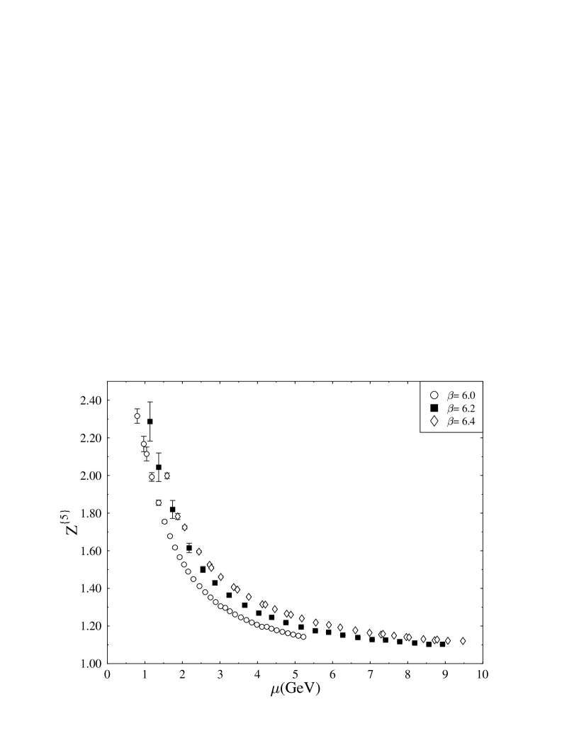
FIG. 1.: The renormalization constant $Z^{\{5\}}$ in the $\overline{\rm MS}$ scheme.

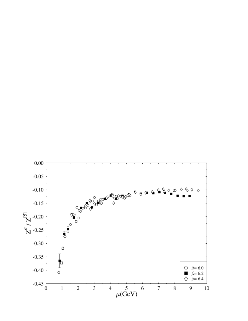
FIG. 2.: The ratio $Z^{\sigma}(a\mu)/Z^{[5]}(a\mu)$.

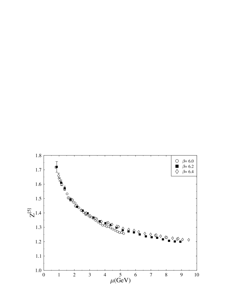
FIG. 3.: The renormalization factor $Z^{[5]}(a\mu)$.

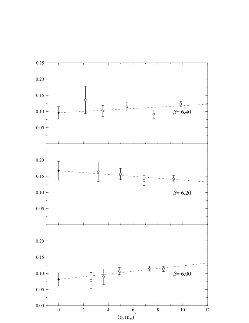
FIG. 4.: Chiral extrapolation of the bare matrix element $a_{2}^{(u)}$ in the proton.

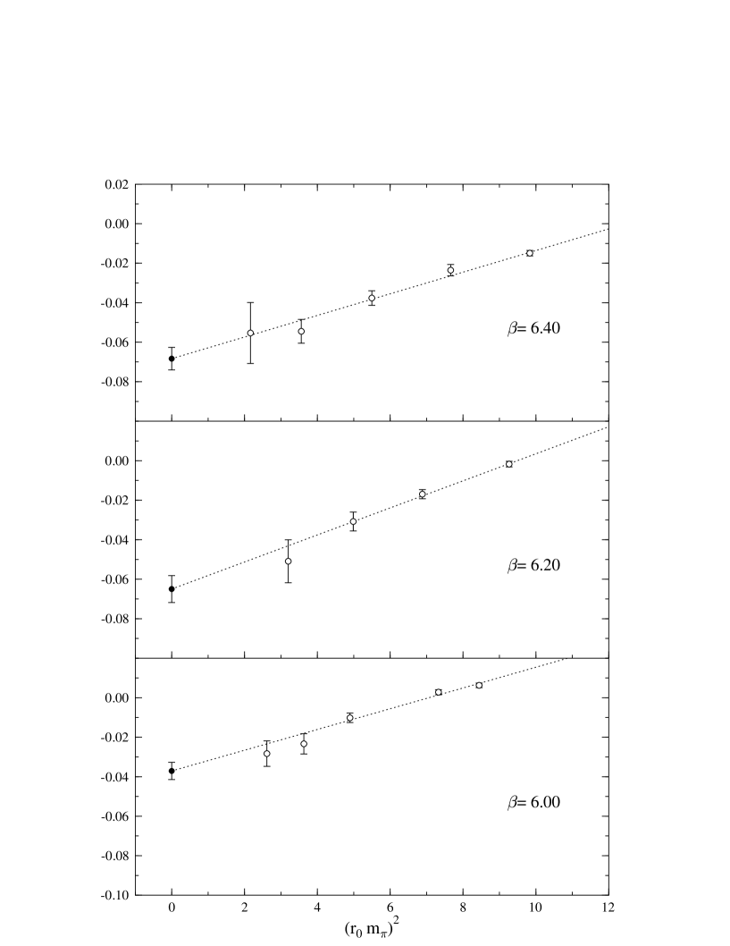
FIG. 5.: Chiral extrapolation of the bare matrix element $d_{2}^{[5]\,(u)}$ in the proton.

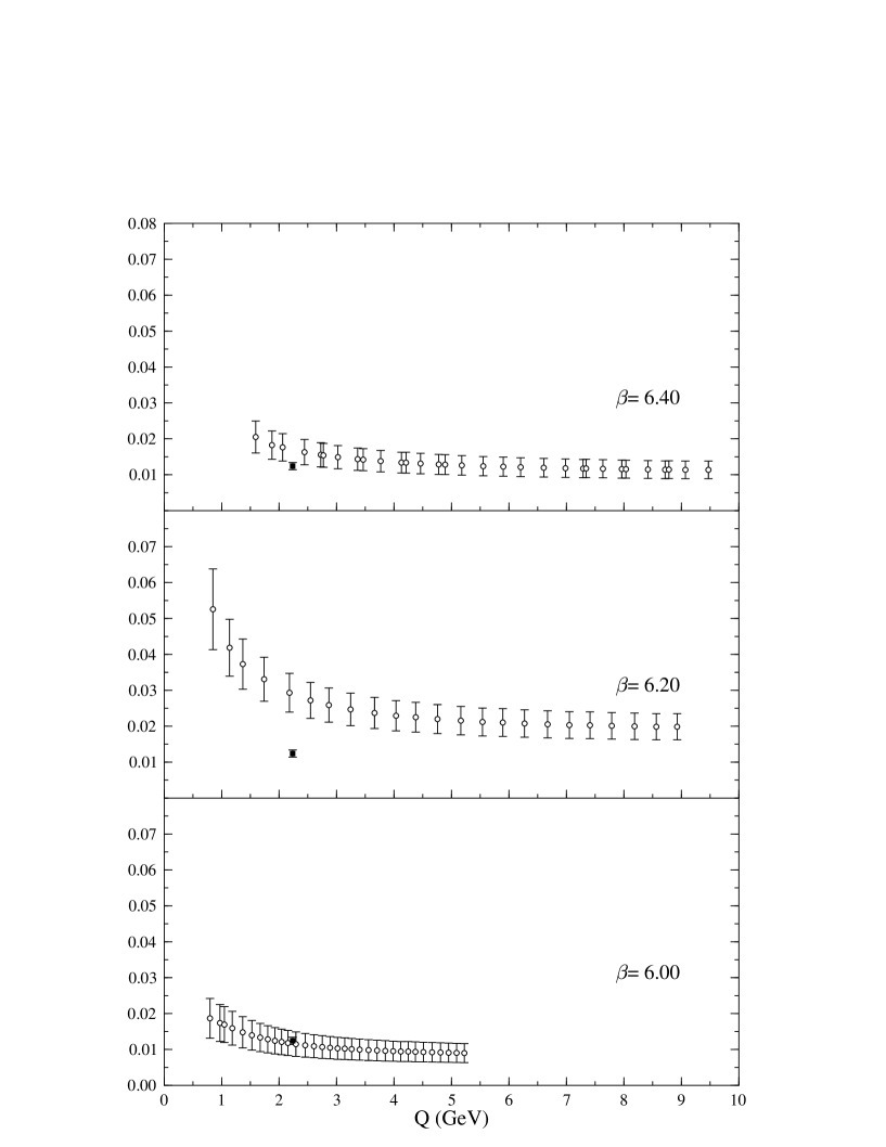
FIG. 6.: The moment $\int_{0}^{1}\mbox{d}xx^{2}g_{1}(x,Q^{2})$ for the proton. The square indicates the experimental value [3].

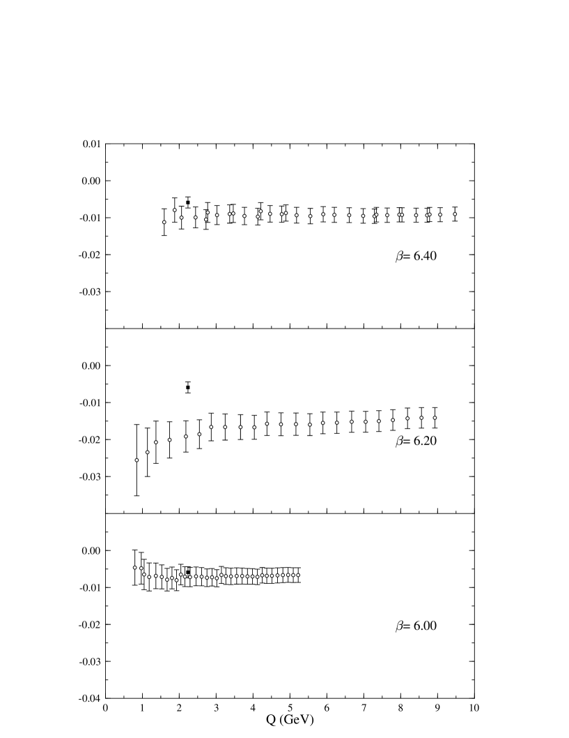
FIG. 7.: The moment $\int_{0}^{1}\mbox{d}xx^{2}g_{2}(x,Q^{2})$ for the proton. The square indicates the experimental value obtained by combining results from [3] and [4].

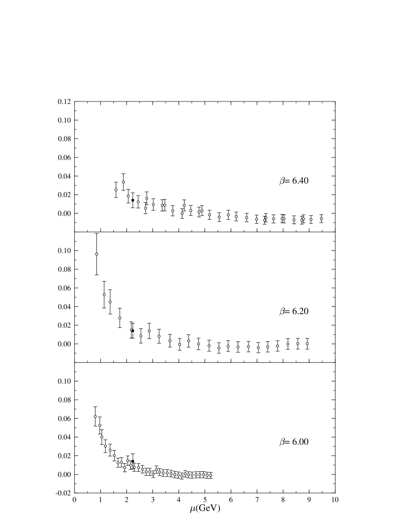
FIG. 8.: The reduced matrix element $d_{2}$ in the proton. The square indicates the experimental value [4].

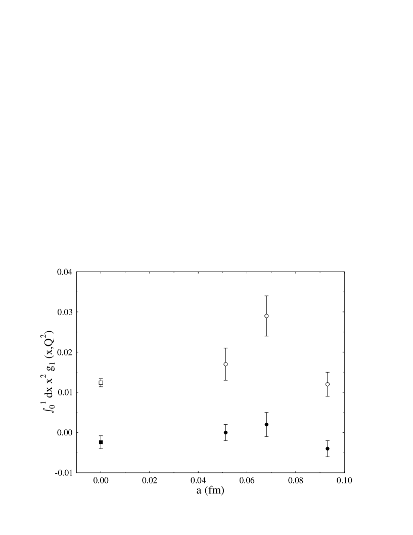
FIG. 9.: The moment $\int_{0}^{1}\mbox{d}xx^{2}g_{1}(x,Q^{2})$ at $Q^{2}=5\,\mbox{GeV}^{2}$ for the proton (open symbols) and the neutron (filled symbols) plotted versus the lattice spacing $a$. The squares at $a=0$ indicate the experimental values [3].

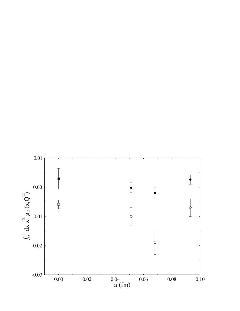
FIG. 10.: The moment $\int_{0}^{1}\mbox{d}xx^{2}g_{2}(x,Q^{2})$ at $Q^{2}=5\,\mbox{GeV}^{2}$ for the proton (open symbols) and the neutron (filled symbols) plotted versus the lattice spacing $a$. The squares at $a=0$ indicate the experimental values obtained by combining results from [3] and [4].

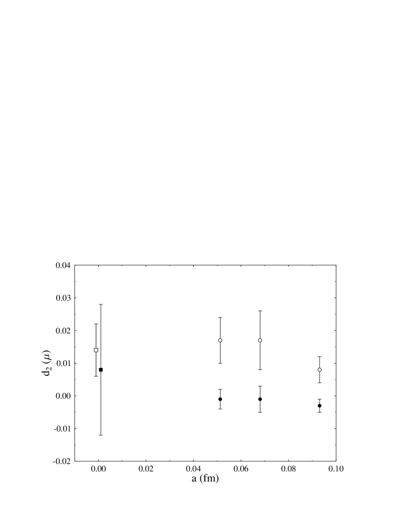
FIG. 11.: The reduced matrix element $d_{2}$ at $\mu^{2}=5\,\mbox{GeV}^{2}$ for the proton (open symbols) and the neutron (filled symbols) plotted versus the lattice spacing $a$. The squares at $a=0$ indicate the experimental values [4]. They are plotted with a slight horizontal offset to avoid overlapping error bars.

REFERENCES

- [1] R.L. Jaffe, Comments Nucl. Part. Phys. 19, 239 (1990); R.L. Jaffe and X. Ji, Phys. Rev. D 43, 724 (1991).
- [2] S. Wandzura and F. Wilczek, Phys. Lett. B 72, 195 (1977).
- [3] K. Abe et al. (E143 collaboration), Phys. Rev. D 58, 112003 (1998).
- [4] P.L. Anthony et al. (E155 collaboration), Phys. Lett. B 458, 529 (1999).
- [5] M. Göckeler, R. Horsley, E.-M. Ilgenfritz, H. Perlt, P. Rakow, G. Schierholz, and A. Schiller, Phys. Rev. D 53, 2317 (1996).
- [6] D. Dolgov, R. Brower, S. Capitani, J.W. Negele, A. Pochinsky, D. Renner, N. Eicker, T. Lippert, K. Schilling, R.G. Edwards, and U.M. Heller, hep-lat/0011010.
- [7] G. Martinelli, C. Pittori, C.T. Sachrajda, M. Testa, and A. Vladikas, Nucl. Phys. B445, 81 (1995).
- [8] K. Jansen, C. Liu, M. Lüscher, H. Simma, S. Sint, R. Sommer, P. Weisz, and U. Wolff, Phys. Lett. B 372, 275 (1996).
- [9] M. Göckeler, R. Horsley, H. Oelrich, H. Perlt, D. Petters, P. Rakow, A. Schäfer, and G. Schierholz, Nucl. Phys. B544, 699 (1999).
- [10] M. Göckeler, R. Horsley, W. Kürzinger, H. Oelrich, P. Rakow, and G. Schierholz, hep-ph/9909253.
- [11] E.V. Shuryak and A.I. Vainshtein, Nucl. Phys. B201, 141 (1982); A.P. Bukhvostov, E.A. Kuraev, and L.N. Lipatov, JETP Lett. 37, 482 (1983); Sov. Phys. JETP 60, 22 (1984); P.G. Ratcliffe, Nucl. Phys. B264, 493 (1986); I.I. Balitsky and V.M. Braun, Nucl. Phys. B311, 541 (1988/89); X. Ji and C. Chou, Phys. Rev. D 42, 3637 (1990).
- [12] J. Kodaira, Y. Yasui, and T. Uematsu, Phys. Lett. B 344, 348 (1995).
- [13] J. Kodaira, Y. Yasui, K. Tanaka, and T. Uematsu, Phys. Lett. B 387, 855 (1996).
- [14] A. Ali, V.M. Braun, and G. Hiller, Phys. Lett. B 266, 117 (1991).
- [15] K. Sasaki, Phys. Rev. D 58, 094007 (1998).
- [16] C. Best, M. Göckeler, R. Horsley, E.–M. Ilgenfritz, H. Perlt, P. Rakow, A. Schäfer, G. Schierholz, A. Schiller, and S. Schramm, Phys. Rev. D 56, 2743 (1997).
- [17] M. Göckeler, R. Horsley, E.-M. Ilgenfritz, H. Perlt, P. Rakow, G. Schierholz, and A. Schiller, Nucl. Phys. B472, 309 (1996).
- [18] M. Baake, B. Gemünden, and R. Oedingen, J. Math. Phys. 23, 944 (1982); J. Mandula, G. Zweig, and J. Govaerts, Nucl. Phys. B228, 109 (1983).
- [19] M. Göckeler, R. Horsley, E.-M. Ilgenfritz, H. Perlt, P. Rakow, G. Schierholz, and A. Schiller, Phys. Rev. D 54, 5705 (1996).
- [20] M. Lüscher, S. Sint, R. Sommer, P. Weisz, and U. Wolff, Nucl. Phys. B491, 323 (1997).
- [21] M. Göckeler, R. Horsley, H. Oelrich, D. Petters, D. Pleiter, P.E.L. Rakow, G. Schierholz, and P. Stephenson, Phys. Rev. D 62, 054504 (2000).
- [22] M. Stratmann, A. Weber, and W. Vogelsang, Phys. Rev. D 53, 138 (1996).
- [23] X. Ji, W. Lu, J. Osborne, and X. Song, hep-ph/0006121.
- [24] S. Capitani, M. Göckeler, R. Horsley, H. Perlt, P.E.L. Rakow, G. Schierholz, and A. Schiller, hep-lat/0007004.
- [25] M. Guagnelli, R. Sommer, and H. Wittig, Nucl. Phys. B535, 389 (1998).